Bayesian Test of Significance for Conditional Independence: The Multinomial Model


Abstract
: Conditional independence tests have received special attention lately in machine learning and computational intelligence related literature as an important indicator of the relationship among the variables used by their models. In the field of probabilistic graphical models, which includes Bayesian network models, conditional independence tests are especially important for the task of learning the probabilistic graphical model structure from data. In this paper, we propose the full Bayesian significance test for tests of conditional independence for discrete datasets. The full Bayesian significance test is a powerful Bayesian test for precise hypothesis, as an alternative to the frequentist’s significance tests (characterized by the calculation of the p-value).
1. Introduction
Barlow and Pereira [1] discussed a graphical approach to conditional independence. A probabilistic influence diagram is a directed acyclic graph (DAG) that helps model statistical problems. The graph is composed of a set of nodes or vertices, which represent the variables, and a set of arcs joining the nodes, which represent the dependence relationships shared by these variables.
The construction of this model helps us understand the problem and gives a good representation of the interdependence of the implicated variables. The joint probability of these variables can be written as a product of their conditional distributions, based on their independence and conditional independence.
The interdependence of the variables [2] is sometimes unknown. In this case, the model structure must be learned from data. Algorithms, such as the IC-algorithm (inferred causation) described in Pearl and Verma [3], have been designed to uncover these structures from the data. This algorithm uses a series of conditional independence tests (CI tests) to remove and direct the arcs, connecting the variables in the model and returning a DAG that minimally (with the minimum number of parameters and without loss of information) represents the variables in the problem.
The problem of constructing the DAG structures based on the data motivates the proposal of new powerful statistical tests for the hypothesis of conditional independence, because the accuracy of the structures learned is directly affected by the errors committed by these tests. Recently proposed structure learning algorithms [4–6] indicate that the results of CI tests are the main source of errors.
In this paper, we propose the full Bayesian significance test (FBST) as a test of conditional independence for discrete datasets. FBST is a powerful Bayesian test for a precise hypothesis and can be used to learn the DAG structures based on the data as an alternative to the CI tests currently in use, such as Pearson’s chi-squared test.
This paper is organized as follows. In Section 2, we review the FBST. In Section 3, we review the FBST for the composite hypothesis. Section 4 gives an example of testing for conditional independence that can be used to construct a simple model with three variables.
2. The Full Bayesian Significance Test
The full Bayesian significance test was presented by Pereira and Stern [7] as a coherent Bayesian significance test for sharp hypotheses. In the FBST, the evidence for a precise hypothesis is computed.
This evidence is given by the complement of the probability of a credible set, called the tangent set, which is a subset of the parameter space in which the posterior density of each of the elements is greater than the maximum of the posterior density over the null hypothesis. This evidence is called the e-value, ev(H), and has many desirable properties as a statistical support. For example, Borges and Stern [8] described the following properties:
- (1)
provides a measure of significance for the hypothesis as a probability defined directly in the original parameter space.
- (2)
provides a smooth measure of the significance, both continuous and differentiable, of the hypothesis parameters.
- (3)
has an invariant geometric definition, independent of the particular parameterization of the null hypothesis being tested or the particular coordinate system chosen for the parameter space.
- (4)
obeys the likelihood principle.
- (5)
requires no ad hoc artifice, such as an arbitrary initial belief ratio between hypotheses.
- (6)
is a possibilistic support function, where the support of a logical disjunction is the maximum support among the support of the disjuncts.
- (7)
provides a consistent test for a given sharp hypothesis.
- (8)
provides compositionality operations in complex models.
- (9)
is an exact procedure, making no use of asymptotic approximations when computing the e-value.
- (10)
allows the incorporation of previous experience or expert opinions via prior distributions.
Furthermore, FBST is an exact test, whereas tests, such as the one presented in Geenens and Simar [9], are asymptotically correct. Therefore, the authors consider that a direct comparison between FBST and such test is not relevant in the context of this paper; considering, as future research, the comparison using small samples, in which case, FBST is still valid.
A more formal definition is given below.
Consider a model in a statistical space described by the triple, (Ξ, Δ, Θ), where Ξ is the sample space, Δ, the family of measurable subsets of Ξ and Θ the parameter space (Θ is a subset of ℜn).
Define a subset of the parameter space, Tφ (tangent set), where the posterior density (denoted by fx) of each element of this set is greater than φ.
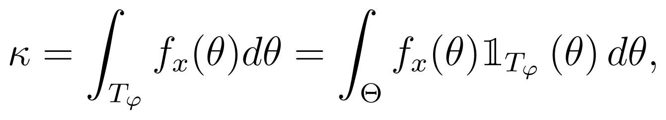
The credibility of Tφ is given by its posterior probability,

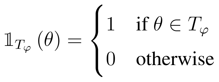
where
 (θ) is the indicator function.

Defining the maximum of the posterior density over the null hypothesis as , with the maximum point at ,
and defining as the tangent set to the null hypothesis, H0, the credibility of T* is κ*.
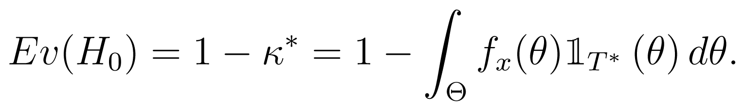
The measure of the evidence for the null hypothesis (called the e-value), which is the complement of the probability of the set T*, is defined as follows:

If the probability of the set, T*, is large, the null set falls within a region of low probability, and the evidence is against the null hypothesis, H0. However, if the probability of T* is small, then the null set is in a region of high probability, and the evidence supports the null hypothesis.
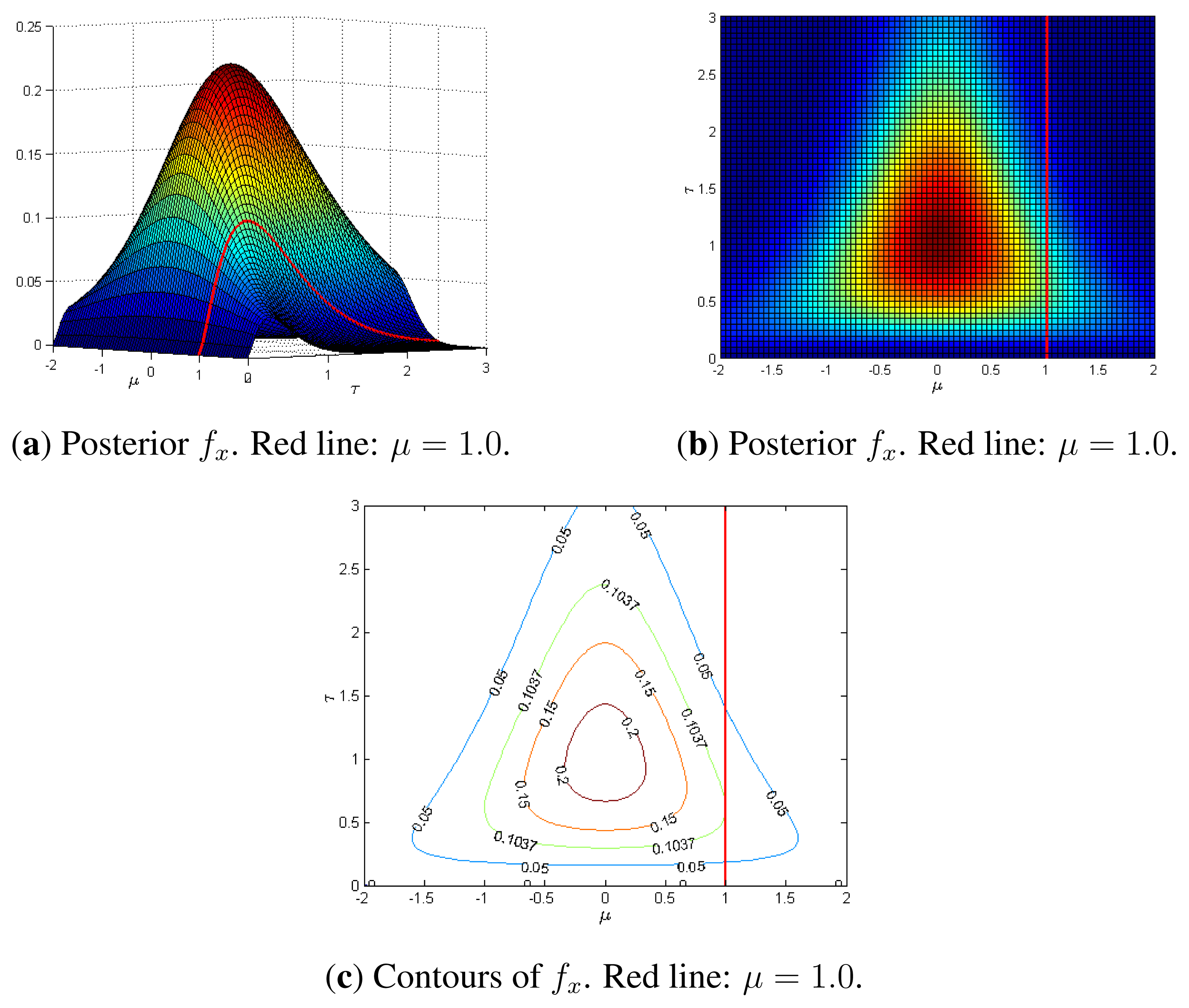
2.1. FBST: Example of Tangent Set
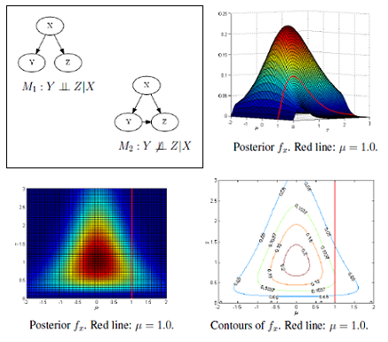
Figure 1 shows the tangent set for a null hypothesis H0 : μ = 1, for the posterior distribution, fx, given bellow, where μ is the mean of a normal distribution and τ is the precision (the inverse of the variance ):
3. FBST: Compositionality
The relationship between the credibility of a complex hypothesis, H, and its elementary constituent, Hj, j = 1, . . . , k, under the full Bayesian significance test, was analyzed by Borges and Stern [8].
For a given set of independent parameters, (θ1, . . . , θk) ∈ (Θ1 × . . . × Θk), a complex hypothesis, H, can be given as follows:
where is a subset of the parameter space, Θj, for j = 1, . . . , k and is constrained to the hypothesis, H, which can be decomposed into its elementary components (hypotheses):
The credibility of H can be evaluated based on the credibility of these components. The evidence in favor of the complex hypothesis, H (measured by its e-value), cannot be obtained directly from the evidence in favor of the elementary components; instead, it must be based on their truth function, Wj (or cumulative surprise distribution), as defined below. For a given elementary component (Hj) of the complex hypothesis, H, is the point of maximum density of the posterior distribution (fx) that is constrained to the subset of the parameter space defined by hypothesis Hj:
The truth function, Wj, is the probability of the parameter subspace (region Rj(v) of the parameter space defined below), where the posterior density is lower than or equal to the value, v:
The evidence supporting the hypothesis, Hj, is given as follows:
The evidence supporting the complex hypothesis can be then described in terms of the truth function of its components as follows.
Given two independent variables, X and Y, if Z = XY, with cumulative distribution functions FZ(z), FX(x) and FY(y), then:
Accordingly, we define a functional product for cumulative distribution functions, namely,
The same result concerning the product of non-negative random variables can be expressed by the Mellin convolution of the probability density functions, as demonstrated by Kaplan and Lin [10], Springer [11] and Williamson [12].
The evidence supporting the complex hypothesis can be then described as the Mellin convolution of the truth function of its components:
The Mellin convolution of two truth functions, W1 ⊗ W2, is the distribution function; see Borges and Stern [8]:
The Mellin convolution W1 ⊗ W2 gives the distribution function of the product of two independent random variables, with distribution functions W1 and W2; see Kaplan and Lin [13] and Williamson [12]. Furthermore, the commutative and associative properties follow immediately for the Mellin convolution,
3.1. Mellin Convolution: Example
An example of a Mellin convolution to find the product of two random variables, Y1 and Y2, both of which have a Log-normal distribution, is given below.
Assume Y1 and Y2 to be continuous random variables, such that:
We denote the cumulative distributions of Y1 and Y2 by W1 and W2, respectively, i.e.,
where fY1 and fY2 are the density functions of Y1 and Y2, respectively. These distributions can be written as a function of two normally distributed random variables, X1 and X2:
We can confirm that the distribution of the product of these random variables (Y1 · Y2) is also Log-normal, using simple arithmetic operations:
The cumulative density function of Y1 · Y2 (W12(y12)) is defined as follows:
where fY1·Y2 is the density function of Y1 · Y2.
In the next section, we show different numerical methods for use in the convolution and condensation procedures, and we apply the results of these procedures to the example given here.
3.2. Numerical Methods for Convolution and Condensation
Williamson and Downs [14] developed the idea of probabilistic arithmetics. They investigated numerical procedures that allow for the computation of a distribution using arithmetic operations on random variables by replacing basic arithmetic operations on numbers with arithmetic operations on random variables. They demonstrated numerical methods for calculating the convolution of probability distributions for a set of random variables.
The convolution for the multiplication of two random variables, X1 and X2 (Z = X1 · X2), can be written using their respective cumulative distribution functions, FX1 and FY2:
The algorithm for the numerical calculation of the distribution of the product of two independent random variables (Y1 and Y2), using their discretized marginal probability distributions (fY1 and fY2) is shown in Algorithm 1 (an algorithm for a discretization procedure is given by Williamson and Downs [14]). The description of Algorithm 1 is given below.
- (1)
The algorithm has as inputs two discrete variables, Y1 and Y2, as well as their respective probabilistic density functions (pdf): fY1 and fY2.
- (2)
The algorithm finds the products (Y1 · Y2 and fY1 · fY2), resulting in N2 bins, if fY1 and fY2 each have N bins.
- (3)
The values of Y1 · Y2 are sorted in increasing order.
- (4)
The values of fY1 · fY2 are sorted according to the order of Y1 · Y2.
- (5)
The cumulative density function (cdf) of the product Y1 · Y2 is found (it has N2 bins).
The numerical convolution of the two distributions with N bins, as described above, returns a distribution with N2 bins. For a sequence of operations, such a large number of bins would be a problem, because the result of each operation would be larger than the input for the operations. Therefore, the authors have proposed a simple method for reducing the size of the output to N bins without introducing further error into the result. This operation is called condensation and returns the upper and lower bounds of each of the N bins for the distribution resulting from the convolution. The algorithm for the condensation process is shown in Algorithm 2. The description of Algorithm 2 is given below.
- (1)
The algorithm has as input a cdf with N2 bins.
- (2)
For each group of N bins (there are N groups of N bins), the value of the cdf at the first bin is taken as the lower bound, and the value of the cdf at the last bin is taken as the upper bound.
- (3)
The algorithm returns a cdf with N bins, where each bin has a lower and an upper bound.

| 1: | procedure Convolution(Y1, Y2, fY1, fY2) | ▹ Discrete pdf of Y1 and Y2 |
| 2: | f ← array(0, size ← n2) | ▹ f and W has n2 bins |
| 3: | W ← array(0, size ← n2) | |
| 4: | y1y2 ← array(0, size ← n2) | ▹ keep Y1 * Y2 |
| 5: | for i ← 1, n do | ▹ f1 and f2 have n bins |
| 6: | for j ← 1, n do | |
| 7: | f [(i − 1) · n + j] ← fY1 [i] · fY2 [j] | |
| 8: | y1y2[(i − 1) · n + j] ← Y1[i] * Y2[j] | |
| 9: | end for | |
| 10: | end for | |
| 11: | sortedIdx ← order(y1y2) | ▹ find order of Y1 * Y2 |
| 12: | f ← f [sortedIdx] | ▹ sort f according to Y1 * Y2 |
| 13: | W [1] ← f [1] | |
| 14: | for i ← k, n2 do | ▹ find cdf of Y1 · Y2 |
| 15: | W [k] ← f [k] | |
| 16: | W [k] ← W [k] +W [k − 1] | |
| 17: | end for | |
| 18: | return W | ▹ Discrete cdf of Y1 · Y2 |
| 19: | end procedure |
| 1: | procedure HorizontalCondensation(W) | ▹ Histogram of a cdf with n2 bins |
| 2: | Wl ← array(0, size ← n) | |
| 3: | Wu ← array(0, size ← n) | |
| 4: | for i ← 1, n do | |
| 5: | Wl [i] ← W [(i − 1) · n + 1] | ▹ lower bound after condensation |
| 6: | Wu [i] ← W [i · n] | ▹ upper bound after condensation |
| 7: | end for | |
| 8: | return [Wl,Wu] | ▹ Histograms with upper/lower bounds |
| 9: | end procedure |
| 1: | procedure VerticalCondensation(W,f,x) | ▹ Histograms of a cdf and pdf, and breaks in the x-axis. |
| 2: | breaks ← [1/n, 2/n, ..., 1] | ▹ uniform breaks in y-axis |
| 3: | Wn ← array (0, size ← n] | |
| 4: | xn ← array (0, size ← n] | |
| 5: | lastbreak ← 1 | |
| 6: | i ← 1 | |
| 7: | for all b ∈ breaks do | |
| 8: | w ← first(W ≥ b) | ▹ find break to create current bin |
| 9: | if W [w] ≠ b then | ▹ if the break is within a current bin |
| 10: | ratio ← (b − W [w − 1])/(W [w] − W [w − 1]) | |
| 11: | ||
| 12: | W [i − 1] ← b | |
| 13: | Wn [i] ← b | |
| 14: | f [i − 1] ← f [w − 1] + ratio · f [w] | |
| 15: | f [i] ← (1 − ratio) · f [w] | |
| 16: | else | |
| 17: | xn [i] ← x [w] | |
| 18: | Wn [i] ← W [w] | |
| 19: | end if | |
| 20: | lastbreak ← b | |
| 21: | i ← i + 1 | |
| 22: | end for | |
| 23: | return [Wn, xn] | ▹ Histograms with upper/lower bounds |
| 24: | end procedure |
3.2.1. Vertical Condensation
Kaplan and Lin [13] proposed a vertical condensation procedure for discrete probability calculations, where the condensation is done using the vertical axis, instead of the horizontal axis, as used by Williamson and Downs [14].
The advantage of this approach is that it provides greater control over the representation of the distribution; instead of selecting an interval of the domain of the cumulative distribution function (values assumed by the random variable) as a bin, we select the interval from the range of the cumulative distribution in [0, 1], which should be represented by each bin.
In this case, it is also possible to focus on a specific region of the distribution. For example, if there is a greater interest in the behavior of the tail of the distribution, the size of the bins can be reduced in this region, consequently increasing the number of bins necessary to represent the tail of the distribution.
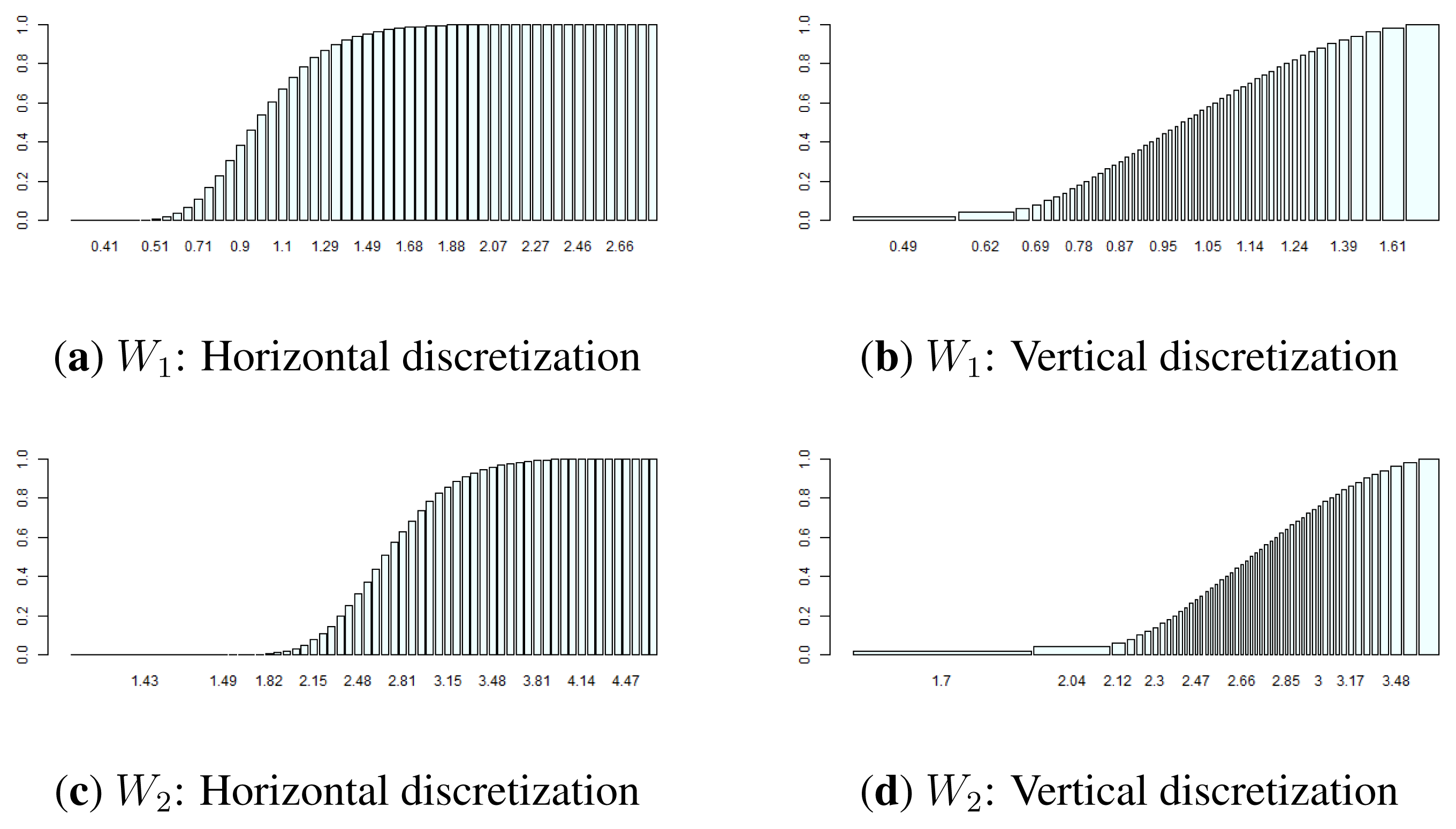
An example of such a convolution that is followed by a condensation procedure using both approaches is given in Section 3.1. For this example, we used discretization and condensation procedures, with the bins uniformly distributed over both axes. At the end of the condensation procedure, using the first approach, the bins are uniformly distributed horizontally (over the sample space of the variable). For the second approach, the bins of the cumulative probability distribution are uniformly distributed over the vertical axis on the interval [0, 1]. Algorithm 3 shows the condensation with the bins uniformly distributed over the vertical axis.
Figure 2 shows the cumulative distribution functions of Y1 and Y2 (Section 3.1) after they have been discretized with bins uniformly distributed over both the x- and y-axes (horizontal and vertical discretizations). Figure 3 shows an example of convolution followed by condensation (based on the example in Section 3.1), using both the horizontal and vertical condensation procedures and the true distribution of the product of two variables with Log-normal distributions.
4. Test of Conditional Independence in Contingency Table Using FBST
We now apply the methods shown in the previous sections to find evidence of a complex null hypothesis of conditional independence for discrete variables.
Given the discrete random variables, X, Y and Z, with X taking values on {1, . . . , k} and Y and Z serving as categorical variables, the test for conditional independence Y ⫫ Z|X can be written as the complex null hypothesis, H:
The hypothesis, H, can be decomposed into its elementary components:
Note that the hypotheses, H1, . . . , Hk, are independent. For each value, x, taken by X, the values taken by variables Y and Z are assumed to be random observations drawn from some distribution p(Y,Z|X = x). Each of the elementary components is a hypothesis of independence in a contingency table. Table 1 shows the contingency table for Y and Z, which take values on {1, . . . , r} and {1, . . . , c}, respectively.
The test of the hypothesis, Hx, can be set up using the multinomial distribution for the cell counts of the contingency table and its natural conjugate prior, i.e., the Dirichlet distribution for the vector of the parameters θx = [θ11x, θ12x, . . . , θrcx].
For a given array of hyperparameters αx = [α11x, . . . , αrcx], the Dirichlet distribution is defined as:
The multinomial likelihood for the given contingency table, assuming the array of observations nx = [n11x, . . . , nrcx] and the sum of the observations , is:
The posterior distribution is thus a Dirichlet distribution, fn(θx):
Under hypothesis Hx, we have Y ⫫ Z|X = x. In this case, the joint distribution is equal to the product of the marginals: p (Y = y, Z = z|X = x) = p (Y = y|X = x) p (Z = z|X = x). We can define this condition using the array of parameters, θx. In this case, we have:
where and .
The elementary components of hypothesis H are as follows:
The point of maximum density of the posterior distribution that is constrained to the subset of the parameter space defined by hypothesis Hx can be estimated using the maximum a posteriori (MAP) estimator under hypothesis Hx (the mode of parameters, θx). The maximum density ( ) is the posterior density evaluated at this point.
where .
The evidence supporting Hx can be written in terms of the truth function, Wx, as defined in Section 3:
The evidence supporting Hx is:
Finally, the evidence supporting the hypothesis of conditional independence (H) is given by the convolution of the truth functions that are evaluated at the product of the points of maximum posterior density, for each component of hypothesis H:
The e-value for hypothesis H can be found using modern mathematical integration methods. An example is given in the next section, using the numerical convolution, followed by the condensation procedures described in Section 3.2. Applying the horizontal condensation method results in an interval for the e-value (found using the lower and upper bounds resulting from the condensation process) and in a single value for the vertical procedure.
4.1. Example of CI Test Using FBST
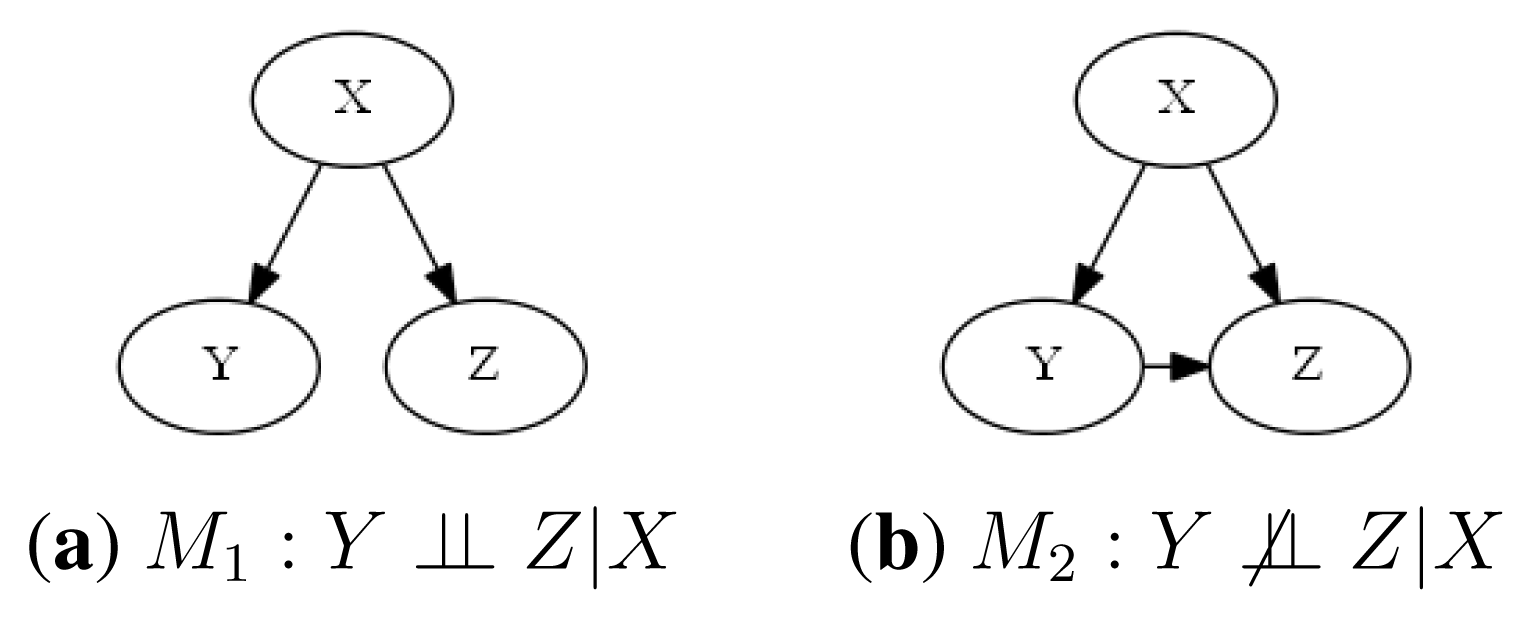
In this section, we describe an example of the CI test using the full Bayesian significance test for conditional independence using samples from two different models. For both models, we test whether the variable, Y, is conditionally independent of Z given X.
Two probabilistic graphical models (M1 and M2) are shown in Figure 4, where the three variables, X, Y and Z, assume values in {1, 2, 3}. In the first model (Figure 4a), the hypothesis of independence H : Y ⫫ Z|X is true, but in the second model (Figure 4b), the same hypothesis is false. The synthetic conditional probability distribution tables (CPTs) used to generate the samples are given in Appendix.
We calculate the intervals for the e-values and compare them, for hypothesis H of conditional independence, for both models: EvM1 (H) and EvM2 (H). The complexity hypothesis, H, can be decomposed into its elementary components:
For each model, 5000 observations were generated; the contingency table of Y and Z for each value of X is shown in Table 2. The hyperparameters of the prior distribution were all set to one, because, in this case, the prior is equivalent to a uniform distribution (from Equation (23)):
The posterior distribution, found using Equations (24) and (25), is then given as follows:
For example, for the given contingency table for Model M1, when X = 2 (Table 2c), the posterior distribution is the following:
The point of highest density, in this example, following the hypothesis of independence (Equations (26) and (28)), was found to be the following:
The truth function and the evidence supporting the hypothesis of independence given X = 2 (hypothesis H2) for Model M1, as given in Equations (29) and (30), are as follows:
We used the methods of numerical integration to find the e-value of the elementary components of hypothesis H (H1,H2 and H3), and the results for each model are given below.
E-values found using horizontal discretization:
E-values found using vertical discretization:
Figure 5 shows the histogram of the truth functions, W1, W2 and W3, for the model, M1 (Y and Z are conditionally independent, given X). In Figure 5a,c,e, 100 bins are uniformly distributed over the x-axis (using the empirical values of min fn(θx) and max fn(θx)). In Figure 5b,d,f, 100 bins are uniformly distributed over the y-axis (each bin represents an increase in 1% in density from the previous bin). The function, Wx, evaluated at the maximum posterior density over the respective hypothesis, , in red, corresponds to the e-values found (e.g., , for the horizontal discretization in Figure 5e).
The evidence supporting the hypothesis of the conditional independence H, as in Equation (31), for each model is as follows:
The convolution follows the commutative property, and the order of the convolutions is therefore irrelevant.
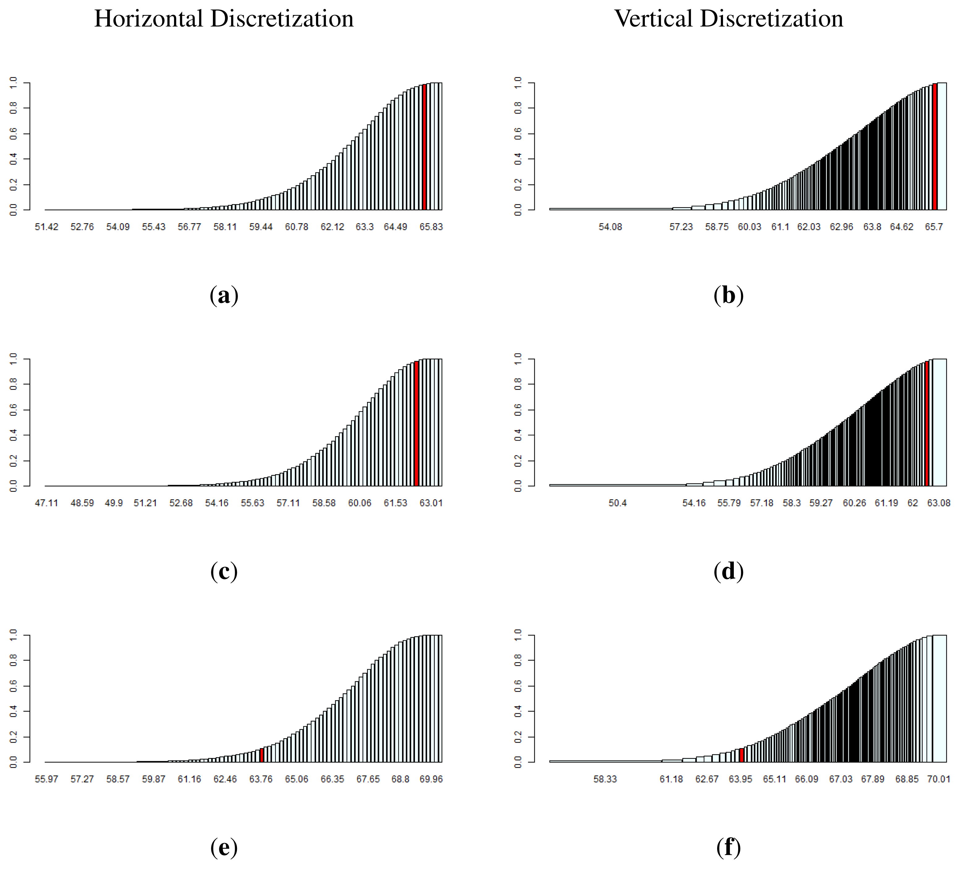
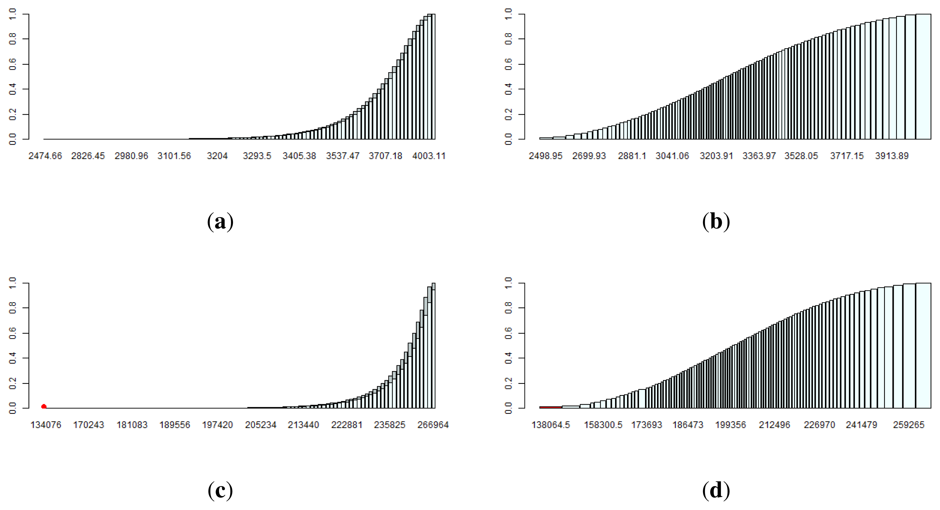
Using the algorithm for numerical convolution described in Algorithm 1, we found the convolution of the truth functions, W1 and W2, resulting in a cumulative function (W12) with 10, 000 bins (1002 bins). We then performed the condensation procedures described in Algorithms 2 and 3 and reduced the cumulative distribution to 100 bins, with lower and upper bounds ( and ) for the horizontal condensation. The results are shown in Figure 6a,b for Model M1 (horizontal and vertical condensations, respectively) and in Figure 7a,b for Model M2.
The convolution of W12 and W3 was followed by their condensation. The results are shown in Figure 6c,d (Model M1) and Figure 7c,d (Model M2).
The e-values supporting the hypothesis of conditional independence for both models are given below.
The intervals for the e-values were found using horizontal discretization and condensation, as follows:
The e-values found using vertical discretization and condensation were as follows:
These results show strong evidence supporting the hypothesis of conditional independence between Y and Z, given X, for Model M1 (using both discretization/condensation procedures). No evidence supporting the same hypothesis for the second model was found. This result is very relevant and promising as a motivation for further studies on the use of FBST as a CI test for the structural learning of graphical models.
5. Conclusions and Future Work
This paper provides a framework for performing tests of conditional independence for discrete datasets using the Full Bayesian Significance Test. A simple application of this test includes examining the structure of a directed acyclic graph given two different models. The result found in this paper suggests that FBST should be considered a good alternative to performing CI tests to uncover the structures of probabilistic graphical models from data.
Future research should include the use of FBST in algorithms to learn the structures of graphs with larger numbers of variables; to increase the capacity for performing these mathematical methods to calculate e-values (because learning DAG structures from data requires an exponential number of CI tests to be performed, each CI test needs to be performed faster); and to empirically evaluate the threshold for e-values to define conditional independence versus dependence. The last of these areas of future exploration should be achieved by minimizing the linear combination of type I and II errors (incorrect rejection of a true hypothesis of conditional independence and failure to reject a false hypothesis of conditional independence).
Acknowledgment
The authors are grateful for the support of IME-USP, to the Coordenação de Aperfeiçoamento de Pessoal de Nível Superior (CAPES), Conselho Nacional de Desenvolvimento Científico e Tecnológico (CNPq) and Fundação de Apoio à Pesquisa do Estado de São Paulo (FAPESP).
Appendix
| (a) CPT of X | |
|---|---|
| X | p(X) |
| 1 | 0.3 |
| 2 | 0.2 |
| 3 | 0.5 |
| (b) CPT of Y given X | |||
|---|---|---|---|
| Y | p(Y|X=1) | p(Y|X=2) | p(Y|X=3) |
| 1 | 0.3 | 0.4 | 0.2 |
| 2 | 0.2 | 0.4 | 0.1 |
| 3 | 0.5 | 0.2 | 0.7 |
| (c) CPT of Z given X | |||
|---|---|---|---|
| Z | p(Z|X=1) | p(Z|X=2) | p(Z|X=3) |
| 1 | 0.5 | 0.1 | 0.6 |
| 2 | 0.4 | 0.1 | 0.1 |
| 3 | 0.1 | 0.8 | 0.3 |
| Z | p(Z|X=1,Y =1) | p(Z|X=1,Y =2) | p(Z|X=1,Y =3) |
|---|---|---|---|
| 1 | 0.5 | 0.1 | 0.6 |
| 2 | 0.4 | 0.1 | 0.1 |
| 3 | 0.1 | 0.8 | 0.3 |
| Z | p(Z|X=2,Y =1) | p(Z|X=2,Y =2) | p(Z|X=2,Y =3) |
|---|---|---|---|
| 1 | 0.2 | 0.4 | 0.8 |
| 2 | 0.2 | 0.3 | 0.1 |
| 3 | 0.6 | 0.3 | 0.1 |
| Z | p(Z|X=3,Y =1) | p(Z|X=3,Y =2) | p(Z|X=3,Y =3) |
|---|---|---|---|
| 1 | 0.1 | 0.5 | 0.2 |
| 2 | 0.2 | 0.4 | 0.6 |
| 3 | 0.7 | 0.1 | 0.2 |
Conflicts of Interest
We certify that there is no conflict of interest regarding the material discussed in the manuscript.
- Author ContributionAll authors made substantial contributions to conception and design, acquisition of data and analysis and interpretation of data; all authors participate in drafting the article or revising it critically for important intellectual content; all authors gave final approval of the version to be submitted and any revised version.
References
- Barlow, R.E.; Pereira, C.A.B. Conditional independence and probabilistic influence diagrams. In Topics in Statistical Dependence; Block, H.W., Sampson, A.R., Savits, T.H., Eds.; Lecture Notes-Monograph Series; Institute of Mathematical Statistics: Beachwood, OH, USA, 1990; pp. 19–33. [Google Scholar]
- Basu, D.; Pereira, C. A. Conditional independence in statistics. Sankhy: The Indian Journal of Statistics 1983, Series A. 371–384. [Google Scholar]
- Pearl, J.; Verma, T.S. A Theory of Inferred Causation; Studies in Logic and the Foundations of Mathematics; Morgan Kaufmann: San Mateo, CA, USA, 1995; pp. 789–811. [Google Scholar]
- Cheng, J.; Bell, D.A.; Liu, W. Learning belief networks from data: An information theory based approach. Proceedings of the sixth International Conference on Information and Knowledge Management, Las Vegas, NV, USA, 10–14 November 1997; pp. 325–331.
- Tsamardinos, I.; Brown, L.E.; Aliferis, C.F. The max-min hill-climbing Bayesian network structure learning algorithm. Mach. Learn 2006, 65, 31–78. [Google Scholar]
- Yehezkel, R.; Lerner, B. Bayesian network structure learning by recursive autonomy identification. J. Mach. Learn. Res 2009, 10, 1527–1570. [Google Scholar]
- Pereira, C.A.B.; Stern, J.M. Evidence and credibility: Full Bayesian significance test for precise hypotheses. Entropy 1999, 1, 99–110. [Google Scholar]
- Borges, W.; Stern, J.M. The rules of logic composition for the Bayesian epistemic e-values. Log. J. IGPL 2007, 15, 401–420. [Google Scholar]
- Geenens, G.; Simar, L. Nonparametric tests for conditional independence in two-way contingency tables. J. Multivar. Anal 2010, 101, 765–788. [Google Scholar]
- Kilicman, A.; Arin, M.R.K. A note on the convolution in the Mellin sense with generalized functions. Bull. Malays. Math. Sci. Soc 2002, 25, 93–100. [Google Scholar]
- Springer, M.D. The Algebra of Random Variables; Wiley: New York, NY, USA, 1979. [Google Scholar]
- Williamson, R.C. Probabilistic Arithmetic. Ph.D Thesis, University of Queensland, Austrilia, 1989. [Google Scholar]
- Kaplan, S.; Lin, J.C. An improved condensation procedure in discrete probability distribution calculations. Risk Anal 1987, 7, 15–19. [Google Scholar]
- Williamson, R.C.; Downs, T. Probabilistic arithmetic. I. Numerical methods for calculating convolutions and dependency bounds. Int. J. Approx. Reason 1990, 4, 89–158. [Google Scholar]


| Z = 1 | Z = 2 | ··· | Z = c | |
|---|---|---|---|---|
| Y = 1 | n11x | n12x | ··· | n1cx |
| Y = 2 | n21x | n22x | ··· | n2cx |
| ··· | ··· | ··· | ··· | ··· |
| Y =r | nr1x | nr2x | ··· | nrcx |
| (a) Model M1 (for X = 1) | ||||
|---|---|---|---|---|
| Z = 1 | Z = 2 | Z = 3 | ||
| Y = 1 | 241 | 187 | 44 | 472 |
| Y = 2 | 139 | 130 | 30 | 299 |
| Y = 3 | 364 | 302 | 70 | 736 |
| 744 | 619 | 144 | 1,507 | |
| (b) Model M2 (for X = 1) | ||||
|---|---|---|---|---|
| Z = 1 | Z = 2 | Z = 3 | ||
| Y = 1 | 228 | 179 | 39 | 446 |
| Y = 2 | 25 | 33 | 211 | 269 |
| Y = 3 | 482 | 75 | 208 | 765 |
| 735 | 287 | 458 | 1,048 | |
| (c) Model M1 (for X = 2) | ||||
|---|---|---|---|---|
| Z = 1 | Z = 2 | Z = 3 | ||
| Y = 1 | 42 | 41 | 323 | 406 |
| Y = 2 | 39 | 41 | 341 | 421 |
| Y = 3 | 15 | 21 | 171 | 207 |
| 96 | 103 | 835 | 1,034 | |
| (d) Model M2 (for X = 2) | ||||
|---|---|---|---|---|
| Z = 1 | Z = 2 | Z = 3 | ||
| Y = 1 | 77 | 85 | 248 | 410 |
| Y = 2 | 165 | 135 | 120 | 420 |
| Y = 3 | 188 | 21 | 24 | 233 |
| 430 | 241 | 392 | 1,036 | |
| (e) Model M1 (for X = 3) | ||||
|---|---|---|---|---|
| Z = 1 | Z = 2 | Z = 3 | ||
| Y = 1 | 282 | 35 | 151 | 468 |
| Y = 2 | 131 | 37 | 79 | 247 |
| Y = 3 | 1,055 | 143 | 546 | 1,744 |
| 1,468 | 215 | 776 | 2,459 | |
| (f) Model M2 (for X = 3) | ||||
|---|---|---|---|---|
| Z = 1 | Z = 2 | Z = 3 | ||
| Y = 1 | 40 | 87 | 354 | 481 |
| Y = 2 | 119 | 104 | 27 | 250 |
| Y = 3 | 305 | 1,049 | 372 | 1,726 |
| 464 | 1,240 | 753 | 2,457 | |
© 2014 by the authors; licensee MDPI, Basel, Switzerland This article is an open access article distributed under the terms and conditions of the Creative Commons Attribution license (http://creativecommons.org/licenses/by/3.0/).
Share and Cite
De Morais Andrade, P.; Stern, J.M.; De Bragança Pereira, C.A. Bayesian Test of Significance for Conditional Independence: The Multinomial Model. Entropy 2014, 16, 1376-1395. https://doi.org/10.3390/e16031376
De Morais Andrade P, Stern JM, De Bragança Pereira CA. Bayesian Test of Significance for Conditional Independence: The Multinomial Model. Entropy. 2014; 16(3):1376-1395. https://doi.org/10.3390/e16031376
Chicago/Turabian StyleDe Morais Andrade, Pablo, Julio Michael Stern, and Carlos Alberto De Bragança Pereira. 2014. "Bayesian Test of Significance for Conditional Independence: The Multinomial Model" Entropy 16, no. 3: 1376-1395. https://doi.org/10.3390/e16031376