Recent Progress in the Definition of Thermodynamic Entropy


Abstract
: The principal methods for the definition of thermodynamic entropy are discussed with special reference to those developed by Carathéodory, the Keenan School, Lieb and Yngvason, and the present authors. An improvement of the latter method is then presented. Seven basic axioms are employed: three Postulates, which are considered as having a quite general validity, and four Assumptions, which identify the domains of validity of the definitions of energy (Assumption 1) and entropy (Assumptions 2, 3, 4). The domain of validity of the present definition of entropy is not restricted to stable equilibrium states. For collections of simple systems, it coincides with that of the proof of existence and uniqueness of an entropy function which characterizes the relation of adiabatic accessibility proposed by Lieb and Yngvason. However, our treatment does not require the formation of scaled copies so that it applies not only to collections of simple systems, but also to systems contained in electric or magnetic fields and to small and few-particle systems.PACS Codes: 05.70.-a thermodynamics1. Introduction
From the origins of classical thermodynamics to the present time, several methods for the definitions of thermodynamic temperature and thermodynamic entropy have been developed. If we exclude the treatments based on statistical mechanics and those which postulate directly the existence and additivity of entropy, as well as the structure of the fundamental relations [1], most of the methods proposed in the literature, up to the most recent contributions, can be divided in three main categories: classical methods, Carathéodory-derived methods, Keenan-school methods.
Classical methods start with the Zeroth-Law of thermodynamics (transitivity of mutual thermal equilibrium) [2,3] and the definition of empirical temperature, then define energy by a suitable statement of the First Law, and finally define thermodynamic temperature and entropy through the Kelvin-Planck statement of the Second Law [4], namely, it is impossible to construct an engine which, operating in a cycle, produces no effect except the lifting of a weight and the cooling of a thermal reservoir.
In their original formulation, classical methods had a logical loop in the definition of energy. In fact, the First Law was stated as follows: in a cycle, the work done by a system is equal to the heat received by the system:
The energy difference between state A2 and state A1 of a system A was defined as the value of Q–W in any process for A from A1 to A2. Clearly, this definition is affected by a logical circularity, because it is impossible to define heat without a previous definition of energy.
The circularity of Equation (1) was understood and resolved in 1909 by Carathéodory [5] who defined an adiabatic process without employing the concept of heat as follows. A vessel is called adiabatic if the state of the system inside it does not change when the bodies present outside the vessel are modified, provided that the vessel remains at rest and retains its original shape and volume. A process such that the system is contained within an adiabatic vessel at every instant of time is called an adiabatic process. Carathéodory stated the First Law as follows: the work performed by a system in any adiabatic process depends only on the end states of the system.
Among the best treatments of thermodynamics by the classical method, we can cite, for instance, those by Fermi [6] and by Zemansky [3]. In these treatments, Carathéodory’s statement of the First Law is adopted.
In his celebrated paper [5], Carathéodory also proposed a new statement of the Second Law and developed a completely new method for the definitions of thermodynamic temperature and entropy. The treatment refers to simple systems, stable equilibrium states, and quasistatic processes, i.e., processes in which the system evolves along a sequence of neighboring stable equilibrium states. A simple system is defined by Carathéodory as a system such that:
- (a)
its stable equilibrium states are determined uniquely by n + 1 coordinates, ξ0, x1, …, xn, where x1, …, xn are deformation coordinates, i.e., coordinates which determine the external shape of the system, while ξ0 is not a deformation coordinate;
- (b)
in every reversible quasistatic process, the work performed by the system is given by:
where p1, …, pn are functions of ξ0, x1, …, xn; and
- (c)
the (internal) energy U of the system, which is defined via the First Law, is additive, i.e., equals the sum of the energies of its subsystems.
Carathéodory stated the Second Law (Axiom II) as follows: in every arbitrarily close neighborhood of a given initial state there exist states that cannot be reached by adiabatic processes. By employing a mathematical theorem on Pfaffian equations, he proved that, on account of the Second Law, there exists a pair of properties, M(ξ0, x1, …, xn) and x0(ξ0, x1, …, xn) such that for every quasistatic process:
Through other assumptions on the conditions for mutual stable equilibrium, which include the Zeroth Law (transitivity of mutual stable equilibrium), Carathéodory proved that there exists a function τ(x0, x1, …, xn) called temperature such that if two systems A and B are in mutual stable equilibrium they have the same temperature. Moreover, by applying the additivity of energy, he proved that there exists a function f (τ), identical for all systems, such that:
where α (·) is another function that varies from system to system.
He then defined thermodynamic temperature T and entropy S respectively as:
where c is an arbitrary constant and Sref is an arbitrary value assigned to the reference state with x0 = x0,ref. Finally, he rewrote Equation (3) in the form:
which, through Equation (2), yields the Gibbs relation for the stable equilibrium states of a simple system.
Carathéodory’s method for the definition of entropy has been the point of origin for several efforts along a similar line of thought. Some authors tried to simplify the treatment and make it less abstract [7–9], while others tried to improve the logical rigor and completeness [10]. Several references on the Carathéodory-derived methods for the definition of entropy are quoted and discussed in a recent paper by Lieb and Yngvason [11].
An alternative method for the treatment of the foundations of thermodynamics was introduced by Keenan [12] and developed by Hatsopoulos and Keenan [13] and by Gyftopoulos and Beretta [14]: It will be called the Keenan-school method. An advantage of this method, with respect to that of Carathéodory, is that the treatment does not employ the concepts of simple system and of quasistatic process so that it applies also to systems contained in electric and magnetic fields and, at least potentially, also to nonequilibrium states. Another step forward introduced by the Keenan school and developed particularly in [14] is the statement of a broad set of operational definitions of the basic concepts of thermodynamics such as those of system, property, state, isolated system, environment of a system, and thermal reservoir. The concept of adiabatic process introduced by Carathéodory is replaced in [14] by the simpler and less restrictive concept of weight process: a process of a system A such that the only net effect in the environment of A is a purely mechanical effect such as, for instance, the raising of a weight in a gravitational field or the displacement of an electric charge in a uniform electrostatic field. The main difference between an adiabatic process and a weight process is that while the former implies a constraint on the whole time evolution of system A and its environment, the latter allows any kind of interaction during the process and sets a constraint only on the end states of the environment of A.
The First Law is stated as follows. Any two states of a system can be the end states of a weight process. Moreover, the work performed by a system in any weight process depends only on the end states of the system [14].
The first part of the statement makes explicit a condition which is almost always employed implicitly when energy is defined through the Carathéodory statement of the First Law. However, the general validity of this condition is questioned in [11]. Indeed, it is possible to release this condition as shown in [15].
A parameter of a system A is defined in [14] as a physical quantity determined by a real number, which describes an overall effect on A of bodies in the environment of A, such as the volume V of a container or the gravitational potential. An equilibrium state of a system A is defined as a stationary state of A which can be reproduced as a stationary state of an isolated system. An equilibrium state of A is called a stable equilibrium state if it cannot be modified in a process which leaves unchanged both the parameters of A and the state of the environment of A. The following statement of the Second Law is employed [14]. Among all the states of a system that have a given value E of the energy and are compatible with a given set of values n of the amounts of constituents and β of the parameters, there exists one and only one stable equilibrium state. Moreover, starting from any state of a system, it is always possible to reach a stable equilibrium state with arbitrarily specified values of amounts of constituents and parameters by means of a reversible weight process.
The second part of this statement of the Second Law is very demanding and should be revised and/or clarified. Indeed, an arbitrary change in composition of a system A (such as one which requires destruction or creation of matter) cannot be obtained by a weight process for A (without the corresponding creation or destruction of antimatter).
The definition of entropy is given by employing two auxiliary quantities, called generalized adiabatic availability and generalized available energy. This method for the definition of entropy has the advantage of emphasizing from the beginning the relation between entropy and the maximum work obtainable in a weight process with a given initial state but has the disadvantage of making the treatment longer and more complex.
In recent years, two novel approaches to the definition of entropy have been introduced by Lieb and Yngvason [11,16,17] and by the present authors [18,19].
The definition of entropy proposed by Lieb and Yngvason is based on the concept of adiabatic accessibility. A state Y is said to be adiabatically accessible from a state X, in symbolic form X ≺ Y, if it is possible to change the state from X to Y by means of an interaction with some device and a weight in such a way that the device returns to its initial state at the end of the process whereas the weight may have changed its position in a gravitational field.
Note that the concept of adiabatic accessibility defined above coincides with that of accessibility by means of a weight process as defined in Reference [14] and not with the adiabatic accessibility considered by Carathéodory.
If X ≺ Y but X is not adiabatically accessible from Y, the symbol X ≺≺ Y is employed. If both X ≺ Y and Y ≺ X, then X is said to be equivalent to Y, X ~ Y. Another key concept in the Lieb-Yngvason approach is that of scaled copy of a system. Let t be any positive real number, Γ a system, and X a state of Γ. The t-scaled copy Γ (t) of Γ is a system such that to every state X of Γ there corresponds a state t X of Γ (t) where the values of all the extensive properties (volume, energy, mole numbers … ) are equal to t times the values they have in state X.
The following axioms on the order relation ≺ are postulated:
- (A1)
Reflexivity. X ~ X.
- (A2)
Transitivity. X ≺ Y and Y ≺ Z implies X ≺ Z.
- (A3)
Consistency. X ≺ Y and X’ ≺ Y’ implies (X, X’) ≺ (Y, Y’), where the pairs of states in brackets are states of the composite system (Γ, Γ’).
- (A4)
Scaling invariance. If X ≺ Y, then t X ≺ t Y for every t > 0.
- (A5)
Splitting and recombination. For 0 < t < 1, X ~ (t X, (1 – t) X).
- (A6)
Stability. If, for some pairs of states X and Y, (X, ɛ Z0) ≺ (Y, ɛ Z1) holds for a sequence of ɛ ’s tending to zero and some states Z0 and Z1, then X ≺ Y.
While Axioms (A1), (A2), and (A3) describe properties that one expects as natural for the adiabatic accessibility relation among states, the other axioms, which refer to scaled copies of a system, limit in effect the validity of the treatment presented in References [11,16] to systems which can be considered as the union of simple systems, each in a stable equilibrium state. For instance, scaled copies cannot be formed for a dielectric system in an electrostatic field nor for a small system with non-negligible, non-local effects and/or near-wall rarefaction or capillarity effects.
Lieb and Yngvason consider a set of stable equilibrium states, which they call state space and denote by Γ, where the following assumption holds:
Comparison hypothesis
Any two states X and Y in Γ are comparable, i.e., either X ≺ Y or Y ≺ X or both.
They prove that in a state space Γ such that the comparison hypothesis holds for Γ and for every scaled copy of Γ, axioms (A1) ÷ (A6) imply the entropy principle stated as follows:
There is a real-valued function on all the stable equilibrium states of all systems (including compound systems), called entropy and denoted by S such that:
- (a)
when X and Y are comparable states, then X ≺ Y if and only if S(X) ≤ S(Y);
- (b)
if X and Y are states of some (possibly different) systems 1 and 2 and if (X, Y) denotes the corresponding state in the state space Γ1 × Γ2 of the composite of the two systems, then the entropy is additive for these states, namely S((X, Y)) = S(X) + S(Y);
- (c)
S is extensive, i.e., for each state X in state space Γ and every integer t > 0, we can write S((t X)) = t S(X) where state (t X) is the scaled copy of X belonging to the t-times scaled copy of Γ, Γ(t).
For a given state spaceΓ, the entropy S can be determined by the following procedure. Let us consider two states in Γ, X0 and X1, such that X0 ≺≺ X1 and, therefore, on account of the entropy principle, S(X0) ≺ S(X1). Let X be a state in Γ, such that X0 ≺ X ≺ X1. Then, it is possible to prove that there exists a unique real number λ between 0 and 1 such that X ~ ((1 – λ) X0, λX1). Once λ has been determined, one has that:
By the procedure explained above and Equation (7) one determines an entropy function on Γ which is unique for every choice of the reference states X0 and X1 or, equivalently, which is determined up to an arbitrary linear transformation: S (X) → a S (X) + B with a > 0. The entropy functions established on the single state space will not, in general, fulfill the additivity for different systems. However, it is possible to prove the following conclusion [16].
Assume that the comparison hypothesis holds for every multiple scaled copy of Γ of the type Γ(t1) × · · · Γ(tN) and let SΓ be an entropy function defined on Γ. Then there exist constants aΓ and B(Γ) such that the function S defined for all the stable equilibrium states of all state spaces Γ(t1) × · · · Γ(tN) by the relation:
for X ∈ Γ, satisfies additivity, i.e., S((X, Y)) = S(X) + S(Y)), extensivity, i.e., S(t X) = t S(X), and is such that whenever X and Y are in the same state space, then X ≺ Y if and only if S(X) ≤ S(Y).
Another result obtained by Lieb and Yngvason in References [11,16] is to prove that the comparison hypothesis can be deduced, for simple systems and their scaled products, as a consequence of nine other axioms, which also imply additional structure of the state spaces and lead, e.g., to the concepts of pressure and temperature and to the concavity of entropy. These results will not be discussed here.
While References [11,16] refer exclusively to stable equilibrium states, very recently Lieb and Yngvason [17] presented an extension of the definition of entropy to a state space Γ̂ which contains also nonequilibrium states (but not all nonequilibrium states) and is such that the comparison hypothesis can be considered as valid in Γ̂. The authors denote by Γ the subset of the stable equilibrium states and assume that in Γ the relation ≺ fulfils Axioms (A1) ÷ (A6), moreover:
- (N1)
in the rest of Γ̂ the relation ≺ fulfils Axioms (A1), (A2), (A3), and (A6); and
- (N2)
for every X ∈ Γ̂ there exist X’, X” ∈ Γ such that X’ ≺ X ≺ X”.
They then prove that the validity of Axioms (A1) ÷ (A6) in Γ, together with the validity of Axioms (N1), (N2) and the comparison hypothesis in the new state space Γ̂ implies the existence and uniqueness (up to a linear transformation) of an entropy function Ŝ in Γ̂, which extends S (i.e., coincides with S in the subset Γ of the stable equilibrium states) and is such that X ≺ Y implies Ŝ (X) ≤ Ŝ(Y) for any two states X and Y in Γ̂.
The contribution provided by Lieb and Yngvason [11,16,17] is an interesting and rigorous analysis of the conditions required for the definition of entropy in a set of states which can also contain nonequilibrium states. However, the definition of entropy along the Lieb-Yngvason method does not suggest a simple direct procedure to measure the entropy difference between any pair of equilibrium or nonequilibrium states. Moreover the method is not applicable, in its present form, to systems contained in external electric or magnetic fields nor to small scale and few particle systems, i.e., systems that do not allow the creation of scaled copies even in their stable equilibrium states.
A different approach to the definition of entropy, inspired by the Keenan-school method but independent of it, was recently developed by the present authors [18,19]. This approach is based on a set of operational definitions of the basic concepts (system, property, state, isolated system, environment of a system, weight process, equilibrium state, stable equilibrium state) very similar to that presented in Reference [14] and on the same statement of the First Law. On the other hand, only the first part of the Second Law statement of Reference [14] is retained. The second part is replaced by a separate assumption, which refers only to closed systems and is not claimed to have a fully general validity. The definition of entropy is not based any more on the concepts of generalized adiabatic availability and of generalized available energy. It is instead obtained directly from the basic assumptions and from the definition of energy. Moreover it is stated for closed systems and extended to open systems [19] only at a later stage of the development. This sharp separation between the treatments of closed and open systems singles out an important conceptual dissimilarity between the meaning of the energy (and entropy) difference between two states of a closed system and that of the energy (and entropy) difference between two states of an open system. Indeed, for a closed system, the energy difference between two states depends only on the unit fixed (once and for all) for energy, and the entropy difference depends only on the units fixed (once and for all) for energy and for thermodynamic temperature. In contrast, for an open system, the energy (and entropy) difference between two states depends also on the choices of the reference states for pure substances and on the energy (and entropy) values assigned to the pure substances in such reference states.
In analogy with Reference [14], the concepts of separable systems and of systems uncorrelated from each other are introduced. Separability is a requirement for the definition of energy: if a system A is a source of long-range force fields for a system B, the energy of A (or of B) cannot be defined. Consider, for instance, two rigid bodies A and B in a gravitational field produced by the systems themselves: while the potential energy of the composite system AB can be defined, that of A or of B cannot. Non-correlation is a requirement imposed for the definition of the thermodynamic entropy, relevant for microscopic or mesoscopic systems, which can exhibit quantum-mechanical correlations with each other.
In this paper, a further development of the method for the definitions of energy and entropy proposed in References [18,19] is presented, with the following improvements. Each of the axioms employed in the treatment is placed in one of two different categories: Postulates, which are statements with a declared fully general validity; Assumptions, which are not claimed to hold necessarily for all systems and states and as such determine the domain of validity of the definitions of energy and of entropy derived from them. In agreement with Lieb and Yngvason [11,16,17], the statement that any two states of a closed system can be the end states of a weight process (i.e., the comparison hypothesis) is not considered as having necessarily a general validity; this statement is not employed in the present treatment. The definition of the energy difference between any pair of states of a closed system is obtained through the following axioms:
Assumption 1
Any pair of states of a closed system A, such that the system is separable from its environment in both states, can be interconnected by a weight polygonal for A.
The concept of weight polygonal, already employed in Reference [15], is defined in Section 3.
Postulate 1
The works done by a system in any two weight polygonals between the same initial and final states are identical.
The definition of entropy is based on two additional Postulates and three additional Assumptions.
Postulate 2
Among all the states of a closed system A such that the constituents of A are contained in a given set of regions of space, there is a stable equilibrium state for every value of the energy EA.
Assumption 2
Starting from any state in which the system is separable from its environment, a closed system A can be changed to a stable equilibrium state with the same energy by means of a zero work weight process for A in which the regions of space occupied by the constituents of A have no net changes.
Postulate 3
There exist systems, called normal systems, whose energy has no upper bound. Starting from any state in which the system is separable from its environment, a normal system A can be changed to a non-equilibrium state with arbitrarily higher energy by means of a weight process for A in which the regions of space occupied by the constituents of A have no net changes.
Assumption 3
There exist normal systems, called thermal reservoirs, which fulfill the following conditions:
- (a)
the regions of space occupied by the constituents are fixed;
- (b)
if R is a thermal reservoir in an arbitrary stable equilibrium state R1 and Rd is an identical copy of R also in arbitrary stable equilbrium state Rd2, not necessarily equal to R1, then R and Rd are in mutual stable equilibrium.
Assumption 4
Every pair of states (A1, A2) of a closed system A, such that A is separable and uncorrelated from its environment in both states, can be interconnected by a reversible standard weight process for AR, where R is an arbitrarily chosen thermal reservoir initially in an arbitrarily chosen stable equilibrium state.
A standard weight process for AR is a weight process for the composite of systems A and R in which the end states of R are stable equilibrium states [18,19] (see definition in Section 4).
It is shown in Section 5 that, if one disregards the conditions of separability and non-correlation (not discussed in References [11,16,17]), one can establish a relation between the domain of validity of the present definition of entropy and that of the definition developed by Lieb and Yngvason. Namely, for systems which allow the creation of scaled copies of their state space when their subsystems are in stable equilibrium states (i.e., collections of simple systems), the domain of validity of the present definition of entropy coincides with the domain of the states in which Lieb and Yngvason prove the existence and uniqueness of an entropy function which characterizes the relation of adiabatic comparability [17]. However, the domain of validity of the present definition of entropy extends also to systems which do not allow the creation of scaled copies even in their stable equilibrium states such as systems contained in electric or magnetic fields, systems with small number of particles for which wall rarefaction effects cannot be neglected, or multi-phase systems for which capillary and interfacial effects are important.
2. Summary of Basic Definitions
We briefly recall here some definitions of the basic concepts of thermodynamics employed in our treatment. A more complete and more detailed set of operational basic definitions can be found in References [18,19].
With the term system we mean a set of material particles, of one or more kinds, such that, at each instant of time, the particles of each kind are contained within a given region of space. If the external surface of the union of the regions of space which contain the particles of the system cannot be crossed by any material particle, the system is called closed.
Any system is endowed with a set of reproducible measurement procedures such that each procedure, if applied at an instant of time t, yields a result which is independent of the previous time evolution of the system. Each procedure of this kind defines a property of the system. The set of all the values of the properties of a system, at a given instant of time, defines the state of the system at that instant.
A system can be in contact with other matter or surrounded by empty space. Moreover, force fields due to external matter can act in the region of space occupied by the system. If, at an instant of time, all the particles of the system are removed from the respective regions of space and brought far away, but a force field is still present in the region of space (previously) occupied by the system, then this force field is called an external force field. An external force field can be either gravitational, or electric or magnetic, or a superposition of the three.
Consider the union ∑ of all the regions of space spanned by a system during its entire time evolution. If no other material particles, except those of the system, are present in ∑ or touch the boundary of ∑, and if the external force field in ∑ is either vanishing or stationary, then we say that the system is isolated. Suppose that an isolated system I can be divided into two subsystems, A and B. Then, we can say that B is the environment of A and vice-versa.
If, at a given instant of time, two systems A and B are such that the force field produced by B is vanishing in the region of space occupied by A and vice-versa, then we say that A and B are separable at that instant. The energy of a system A is defined only for the states of A such that A is separable from its environment.
If, at a given instant of time, two systems A and B are such that the outcomes of the measurements performed on B are statistically independent of those of the measurements performed on A, and vice-versa, we say that A and B are uncorrelated from each other at that instant. The entropy of a system A is defined only for the states of A such that A is separable and uncorrelated from its environment.
We call process of a system A from state A1 to state A2 a time evolution (AB)1 → (AB)2 of the isolated system AB from (AB)1 (with A in state A1) to (AB)2 (with A in state A2), where B is the environment of A. A process of A is reversible if the isolated system AB can undergo a time evolution (AB)2 → (AB)1 which restores it in its initial state (AB)1 and is called the reverse of (AB)1 → (AB)2. A process of a system A is called a cycle for A if the final state A2 coincides with the initial state A1. A cycle for A is not necessarily a cycle for AB.
An elementary mechanical system is a system such that the only admissible change of state for it is a space translation in a uniform external force field. An example is a particle which can only change its height in a uniform external gravitational field. A process of a system A from state A1 to A2, such that both at A1 and at A2 system A is separable from its environment, is called a weight process for A if the only net effect of the process in the environment of A is the change of state of an elementary mechanical system. We call work done by a system A in a weight process for A from A1 to A2, denoted by , the corresponding change in potential energy of the elementary mechanical system. The opposite of , denoted by , is called work received by A in the process.
An equilibrium state of a system is a state such that the system is separable and the state does not vary with time and can be reproduced while the system is isolated. An equilibrium state of a closed system A in which A is uncorrelated from its environment B is called a stable equilibrium state if it cannot be changed to a different state in which A is separable and uncorrelated from its environment by a process such that neither the regions of space where the constituents of A are contained nor the state of the environment B of A have net changes. Two systems, A and B, are in mutual stable equilibrium if the composite system AB (i.e., the union of both systems) is in a stable equilibrium state.
3. Definition of Energy for a Closed System
Weight polygonal and work in a weight polygonal
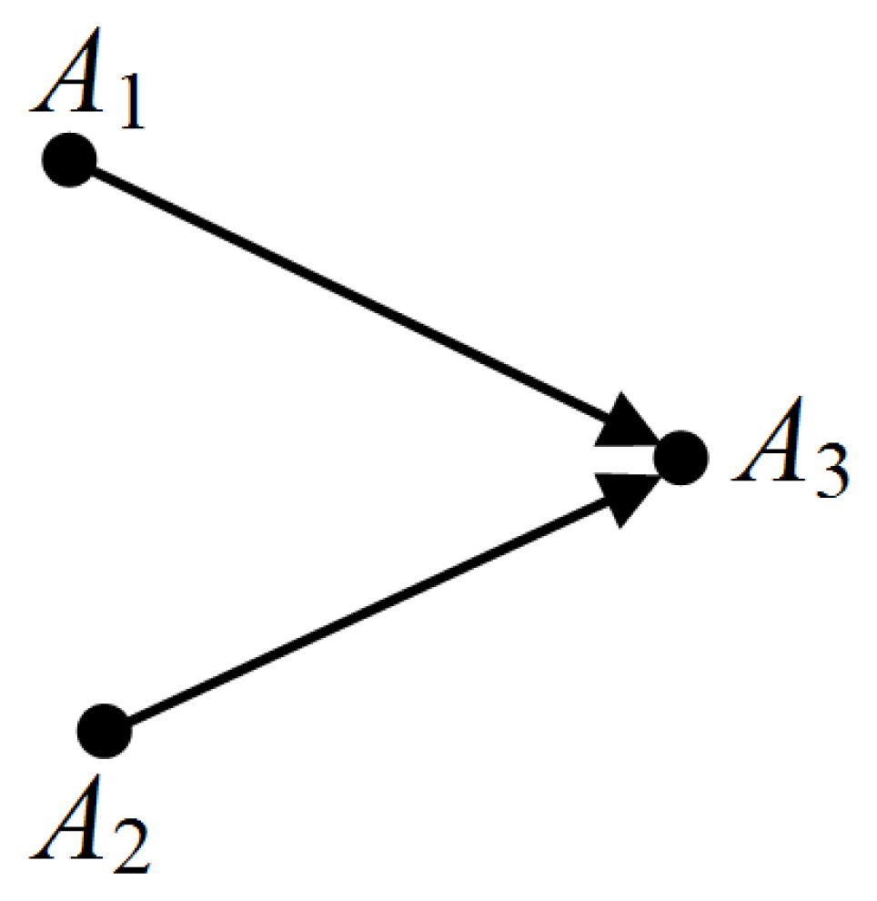
Consider an ordered set of n + 2 states of a closed system A, (A1, Ai1, Ai2, …, Ain-1, Ain, A2), such that in each of these states A is separable from its environment. If n + 1 weight processes exist, which interconnect A1 and Ai1, Ai1 and Ai2, …, Ain-1 and Ain, An and A2, regardless of the direction of each process, we say that A1 and A2 can be interconnected by a weight polygonal. For instance, if weight processes A1 → A3 and A2 → A3 exist for A, we say that A1 → A3 ← A2 is a weight polygonal for A from A1 to A2. We call work done by A in a weight polygonal from A1 to A2 the sum of the works done by A in the weight processes with direction from A1 to A2 and the opposites of the works done by A in the weight processes with direction from A2 to A1 [15]. The work done by A in a weight polygonal from A1 to A2 will be denoted by ; its opposite will be called work received by A in a weight polygonal from A1 to A2 and will be denoted by . Clearly, for a given weight polygonal, . In the example of weight polygonal A1 → A3 ← A2 sketched in Figure 1, one has that:
Assumption 1
Every pair of states (A1, A2) of a closed system A, such that A is separable from its environment in both states, can be interconnected by means of a weight polygonal for A.
Postulate 1
The works done by a system in any two weight polygonals between the same initial and final states are identical.
Comment
In Reference [15] it is proved that, in sets of states where sufficient conditions of interconnectability by weight processes hold, Postulate 1 can be proved as a consequence of the traditional form of the First Law, which concerns weight processes (or adiabatic processes).
Definition of energy for a closed system and proof that it is a property
Let (A1, A2) be any pair of states of a closed system A, such that A is separable from its environment in both states. We call the energy difference between states A2 and A1 the work received by A in any weight polygonal from A1 to A2 expressed as:
Assumption 1 and Postulate 1 yield the following consequences:
- (a)
the energy difference between two states A2 and A1 depends only on the states A1 and A2;
- (b)
(additivity of energy differences) consider a pair of states (AB)1 and (AB)2 of a composite system AB, where both A and B are closed and denote by A1, B1 and A2, B2 the corresponding states of A B; then, if A, B and AB are separable from their environment in the states considered:
- (c)
(energy is a property) let A0 be a reference state of a system A, in which A is separable from its environment, to which we assign an arbitrarily chosen value of energy ; the value of the energy of A in any other state A1 in which A is separable from its environment is determined uniquely by:
where is the work received by A in any weight polygonal for A from A0 to A1;
- (d)
energy is defined for every set of states of any closed system A in which A is separable from its environment and Assumption 1 holds.
Simple proofs of these consequences can be found in Section 5 of Reference [15] and will not be repeated here.
Comment
Since the energy of A is defined only when A is separable from its environment, in the following we will consider as understood that A is separable from its environment in every state in which the energy of A is defined.
4. Definition of entropy for a closed system
Postulate 2
Among all the states of a closed system A such that the constituents of A are contained in a given set of regions of space, there is a stable equilibrium state for every value of the energy EA.
Assumption 2
Starting from any state in which the system is separable from its environment, a closed system A can be changed to a stable equilibrium state with the same energy by means of a zero work weight process for A in which the regions of space occupied by the constituents of A have no net changes.
Lemma 1. Uniqueness of the stable equilibrium state for a given value of the energy
There can be no pair of different stable equilibrium states of a closed system A with identical regions of space occupied by the constituents of A and the same value of the energy EA.
Proof
Since A is closed and in any stable equilibrium state it is separable and uncorrelated from its environment, if two such states existed, by Assumption 2 the system could be changed from one to the other by means of a zero-work weight process, with no change of the regions of space occupied by the constituents of A and no change of the state of the environment of A. Therefore, neither would satisfy the definition of stable equilibrium state.
Postulate 3
There exist systems, called normal systems, whose energy has no upper bound. Starting from any state in which the system is separable from its environment, a normal system A can be changed to a non-equilibrium state with arbitrarily higher energy by means of a weight process for A in which the regions of space occupied by the constituents of A have no net changes.
Comments
Exceptions to this hypothesis are special systems, such as spin systems or systems that can access only a finite number of energy levels, for which the admissible values of the energy are bounded within a finite range. The additivity of energy implies that the union of two or more normal systems, each separable from its environment, is a normal system to which Postulate 3 applies. In traditional treatments of thermodynamics, Postulate 3 is not stated explicitly but is used, for example, when one states that any amount of work can be transferred to a thermal reservoir by a stirrer.
Theorem 1. Impossibility of a Perpetual Motion Machine of the Second Kind (PMM2)
If a normal system A is in a stable equilibrium state, it is impossible to lower its energy by means of a weight process for A in which the regions of space occupied by the constituents of A have no net change.
Proof
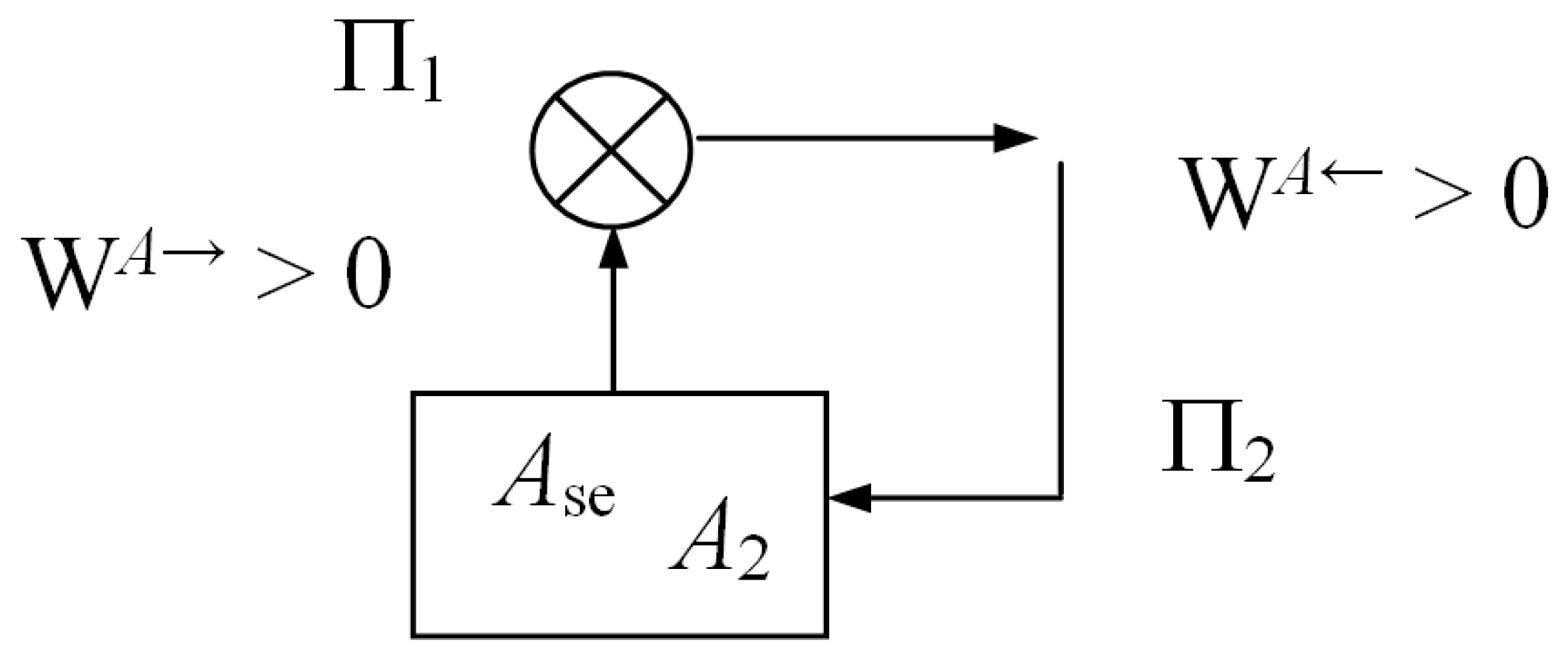
(See sketch in Figure 2). Suppose that, starting from a stable equilibrium state Ase of A, by means of a weight process Π1 with positive work WA→ = W > 0, the energy of A is lowered and the regions of space occupied by the constituents of A have no net change. On account of Postulate 3, it would then be possible to perform a weight process Π2 for A in which the regions of space occupied by the constituents of A have no net change, the weight M is restored to its initial state so that the positive amount of energy WA← = W > 0 is supplied back to A, and the final state of A is a nonequilibrium state, namely, a state clearly different from Ase. Thus, the composite zero-work weight process (Π1, Π2) would violate the definition of stable equilibrium state.
Systems in mutual stable equilibrium
We say that two systems A and B, each in a stable equilibrium state, are in mutual stable equilibrium if the composite system AB is in a stable equilibrium state.
Assumption 3
There exist normal systems, called thermal reservoirs, which fulfill the following conditions:
- (a)
the regions of space occupied by the constituents are fixed;
- (b)
if R is a thermal reservoir in an arbitrary stable equilibrium state R1 and Rd is an identical copy of R also in arbitrary stable equilibrium state Rd2, not necessarily equal to R1, then R and Rd are in mutual stable equilibrium.
Comment
Every normal single-constituent system without internal boundaries and applied external fields, and with a number of particles of the order of one mole (so that the simple system approximation as defined in page 263 of Reference [14] applies), when restricted to a fixed region of space of appropriate volume and to the range of energy values corresponding to the so-called triple-point stable equilibrium states, is an excellent approximation of a thermal reservoir.
Indeed, for a system of this kind, when three different phases (such as, solid, liquid and vapor) are present, two stable equilibrium states with different energy values have, with an extremely high approximation, the same temperature (here not yet defined) and, thus, fulfill the condition for the mutual stable equilibrium of the system and a copy thereof.
The existence of thermal reservoirs has been implicitly assumed in almost every traditional treatment of thermodynamics. It has been a basic assumption in treatments of the physics of open quantum systems [20], fluctuation theory [21], quantum measurement [22], and thermodynamics in the quantum regime [23].
Reference thermal reservoir
A thermal reservoir chosen once and for all is called a reference thermal reservoir. To fix ideas, we choose water as the constituent of our reference thermal reservoir, i.e., sufficient amounts of ice, liquid water, and water vapor at triple point conditions.
Standard weight process
Given a pair of states (A1, A2) of a closed system A and a thermal reservoir R, we call standard weight process for AR from A1 to A2 a weight process for the composite system AR in which the end states of R are stable equilibrium states. We denote by (A1R1 → A2R2)sw a standard weight process for AR from A1 to A2 and by the corresponding energy change of the thermal reservoir R.
Assumption 4
Every pair of states (A1, A2) of a closed system A, such that A is separable and uncorrelated from its environment in both states, can be interconnected by a reversible standard weight process for AR, where R is an arbitrarily chosen thermal reservoir initially in an arbitrarily chosen stable equilibrium state.
Theorem 2
For a given closed system A and a given thermal reservoir R, among all the standard weight processes for AR between a given pair of states (A1, A2) of A in which A is separable and uncorrelated from its environment, the energy change of the thermal reservoir R has a lower bound which is reached if and only if the process is reversible.
Proof
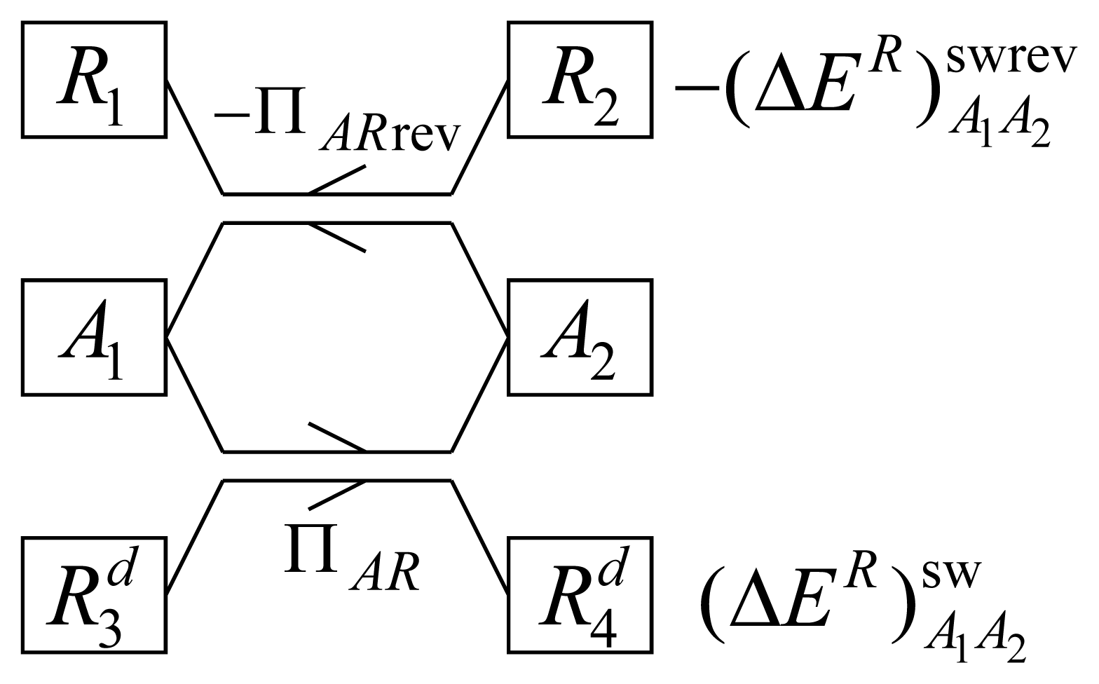
Let ΠAR denote a standard weight process for AR from A1 to A2, and ΠAR rev a reversible one; the energy changes of R in processes ΠAR and ΠAR rev are, respectively, and . With the help of Figure 3, we will prove that regardless of the initial state of R:
- (a)
;
- (b)
if also ΠAR is reversible, then ;
- (c)
if , then also ΠAR is reversible.
Proof of (a)
Let us denote by R1 and R2 the initial and the final states of R in process ΠAR rev. Let us denote by Rd the duplicate of R which is employed in process ΠAR, and by and the initial and the final states of Rd in this process. Let us suppose ab absurdo that , and consider the composite process (−ΠAR rev, ΠAR), where −−ΠAR rev is a reverse of ΠAR rev. This process would be a weight process for RRd in which, starting from the stable equilibrium state , the energy of RRd is lowered and the regions of space occupied by the constituents of RRd have no net changes, in contradiction to Theorem 1. Therefore, .
Proof of (b)
If ΠAR is reversible too, then, in addition to , the relation must hold too. Otherwise, the composite process (ΠAR rev, ΠAR) would be a weight process for RRd in which, starting from the stable equilibrium state , the energy of RRd is lowered and the regions of space occupied by the constituents of RRd have no net changes, in contradiction to Theorem 1. Therefore, .
Proof of (c)
Let ΠAR be a standard weight process for AR, from A1 to A2, such that , and let R1 be the initial state of R in this process. Let ΠAR rev be a reversible standard weight process for AR, from A1 to A2, with the same initial state R1 of R. Thus, coincides with R1 and coincides with R2. The composite process (ΠAR, −ΠAR rev) is a cycle for the isolated system ARB, where B is the environment of AR. As a consequence, ΠAR is reversible, because it is a part of a cycle of the isolated system ARB.
Theorem 3
Let R′ and R″ be any two thermal reservoirs and consider the energy changes, and respectively, in the reversible standard weight processes and , where (A1, A2) is an arbitrarily chosen pair of states of any closed system A, such that A is separable and uncorrelated from its environment in both states. Then the ratio
- (a)
is positive;
- (b)
depends only on R′ and R″, i.e., it is independent of (i) the initial stable equilibrium states of R′ and R″, (ii) the choice of system A, and (iii) the choice of states A1 and A2.
Proof of (a)
With the help of Figure 4, let us suppose that . Then, cannot be zero. In fact, in that case the composite process (ΠAR′, −ΠAR″), which is a cycle for A, would be a weight process for R′ in which, starting from the stable equilibrium state R′1, the energy of R′ is lowered and the regions of space occupied by the constituents of R′ have no net changes, in contradiction to Theorem 1. Moreover, cannot be positive. In fact, if it were positive, the work performed by R′R″ as a result of the overall weight process (ΠAR′, −ΠAR″) for R′R″ would be:
where both terms are positive. After the process (ΠAR′, −ΠAR″), on account of Postulate 3 and Assumption 2, one could perform a weight process ΠR′ for R″ in which a positive amount of energy equal to is given back to R″ and the latter is restored to its initial stable equilibrium state. As a result, the composite process (ΠAR′, ΠAR″, ΠR″) would be a weight process for R′ in which, starting from the stable equilibrium state R′1, the energy of R′ is lowered and the regions of space occupied by the constituents of R′ have no net changes, in contradiction to Theorem 1. Therefore, the condition implies .
Let us suppose that . Then, for process − ΠAR′ one has that . By repeating the previous argument, one proves that for process ΠAR″ one has that . Therefore, for process ΠAR″ one has that .
Proof of (b)
Choose a pair of states (A1, A2) of a closed system A such that A is separable and uncorrelated from its environment and consider the reversible standard weight process ΠAR′ = (A1R1′ → A2R2′)swrev for AR′ with R′ initially in state R′1 and the reversible standard weight process ΠAR″ = (A1R1″ → A2R2″)swrev for AR″ with R″ initially in state R″1. Then choose a pair of states (A′1, A′2) of another closed system A′ such that A′ is separable and uncorrelated from its environment and consider the reversible standard weight process ΠA′R′ = (A1′R1′ → A2′R2′)swrev for A′R′ with R′ initially in state R′1 and the reversible standard weight process ΠA′R″ = (A1′R1″ → A2′R2″)swrev for A′R″ with R″ initially in state R″1.
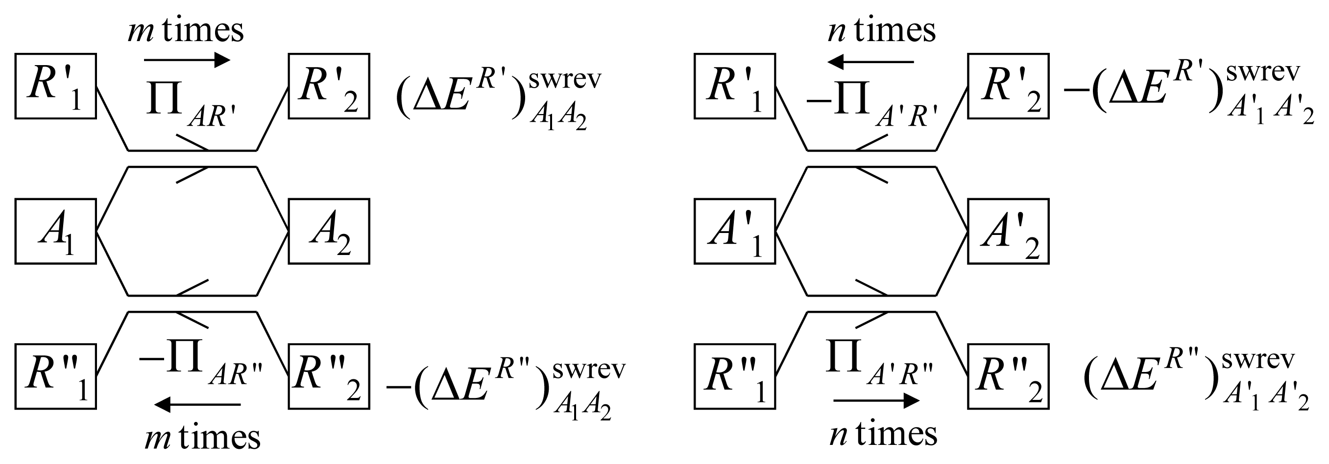
With the help of Figure 5, we will prove that the changes in energy of the reservoirs in these processes obey the relation:
Let us assume: and , which implies, on account of part (a) of the proof, that and . This is not a restriction, because it is possible to reverse the processes under consideration.
Now, as is well known, any real number can be approximated with arbitrarily high accuracy by a rational number. Therefore, we will assume that the energy changes and are rational numbers so that whatever is the value of their ratio, there exist two positive integers m and n such that , i.e.:
As sketched in Figure 5, let us consider the composite processes ΠA and ΠA′ defined below.ΠA is the following composite weight process for the composite system AR′R″: starting from the initial state R′1 of R′ and R″2 of R″, system A is brought from A1 to A2 by a reversible standard weight process for AR′ and then from A2 to A1 by a reversible standard weight process for AR″; whatever the new states of R′ and R″ are, again system A is brought from A1 to A2 by a reversible standard weight process for AR′ and back to A1 by a reversible standard weight process for AR″ until the cycle for A is repeated m times. Similarly, ΠA′ is a composite weight process for the composite system A′R′R″ whereby starting from the end states of R′ and R″ reached by process ΠA, system A′ is brought from A′1 to A′2 by a reversible standard weight process for A′R″; then from A′2 to A′1 by a reversible standard weight process for A′R′; and so on until the cycle for A′ is repeated n times.
Clearly, the whole composite process (ΠA, ΠA′) is a cycle for AA′. Moreover, it is a cycle also for R′. In fact, on account of Theorem 2, the energy change of R′ in each process ΠAR′ is equal to , regardless of its initial state, and in each process −ΠA′R′ is equal to . Therefore, the energy change of R′ in the whole composite process (ΠA, ΠA′) is and equals zero on account of Equation (15). As a result, after (ΠA, ΠA′), reservoir R′ has been restored to its initial state so that (ΠA, ΠA′) is a reversible weight process for R″.
Again, on account of Theorem 2, the overall energy change of R″ in the whole composite process is . If this quantity were negative, Theorem 1 would be violated. If this quantity were positive, Theorem 1 would also be violated by the reverse of the process, (−ΠA, −ΠA′). Therefore, the only possibility is that , i.e.:
Finally, taking the ratio of Equations (15) and (16), we obtain Equation (14) which is our conclusion.
Temperature of a thermal reservoir
Let R be a given thermal reservoir and R0 a reference thermal reservoir. Select an arbitrary pair of states (A1, A2) of a closed system A such that A is separable and uncorrelated from its environment in both states and consider the energy changes and in two reversible standard weight processes from A1 to A2, one for AR and the other for AR0, respectively. We call the temperature of R the positive quantity:
where TR0 is a positive constant associated arbitrarily with the reference thermal reservoir R0.
Clearly, the temperature TR of R is defined only up to the arbitrary multiplicative constant TR0. If for R0 we select a thermal reservoir consisting of ice, liquid water, and water vapor at triple-point conditions and we set TR0 = 273.16 K, we obtain the Kelvin temperature scale.
Corollary 1
The ratio of the temperatures of two thermal reservoirs, R′ and R″, is independent of the choice of the reference thermal reservoir and can be measured directly as:
where and are the energy changes of R′ and R″ in two reversible standard weight processes, one for AR′ and the other for AR″, which interconnect the same pair of states (A1, A2) such that A is separable and uncorrelated from its environment in both states.
Proof
Let be the energy change of the reference thermal reservoir R0 in any reversible standard weight process for AR0 which interconnects the same states (A1, A2) of A. From Equation (17) we have that:
so that the ratio TR′/TR″ is given by Equation (18).
Corollary 2
Let (A1, A2) be any pair of states of a closed system A such that A is separable and uncorrelated from its environment in both states and let be the energy change of a thermal reservoir R with temperature TR in any reversible standard weight process for AR from A1 to A2. Then, for the given system A, the ratio depends only on the pair of states (A1, A2), i.e., it is independent of the choice of reservoir R and of its initial stable equilibrium state R1.
Proof
Let us consider two reversible standard weight processes from A1 to A2, one for AR′ and the other for AR″, where R′ is a thermal reservoir with temperature TR′ and R″ is a thermal reservoir with temperature TR″. Then, Equation (18) yields:
Definition of entropy for a closed system and proof that it is a property
Let (A1, A2) be any pair of states of a closed system A such that A is separable and uncorrelated from its environment in both states, and let R be an arbitrarily chosen thermal reservoir placed in the environment B of A. We call the entropy difference between A2 and A1 the quantity:
where is the energy change of R in any reversible standard weight process for AR from A1 to A2 and TR is the temperature of R. On account of Corollary 2, the right hand side of Equation (21) is determined uniquely by states A1 and A2.
Let A0 be a reference state of A in which A is separable and uncorrelated from its environment and assign to A0 an arbitrarily chosen value of the entropy. Then, the value of the entropy of A in any other state A1 of A in which A is separable and uncorrelated from its environment is determined uniquely by the equation:
where is the energy change of R in any reversible standard weight process for AR from A0 to A1 and TR is the temperature of R.
Therefore, entropy is a property of any closed system A, defined in every set of states of A where Assumptions 2 and 4 hold.
Theorem 4. Additivity of entropy differences
Consider the pair of states (C1 = A1B1, C2 = A2 B2) of the composite system C = AB such that A and B are closed, A is separable and uncorrelated from its environment in both states A1 and A2, and B is separable and uncorrelated from its environment in both states B1 and B2. Then:
Proof
Let us choose a thermal reservoir R with temperature TR and consider the composite process (ΠAR, ΠBR) where ΠAR is a reversible standard weight process for AR from A1 to A2, while ΠBR is a reversible standard weight process for BR from B1 to B2. The composite process (ΠAR, ΠBR) is a reversible standard weight process for CR from C1 to C2 in which the energy change of R is the sum of the energy changes in the constituent processes ΠAR and ΠBR, i.e., . Therefore:
Equation (24) together with the definition of the entropy difference, Equation (21), yield Equation (23).
Comment
As a consequence of Theorem 4, if the values of entropy are chosen so that they are additive over the subsystems in their reference states, the entropy of a composite system is equal to the sum of the entropies of the constituent subsystems.
Theorem 5
Let (A1, A2) be any pair of states of a closed system A such that A is separable and uncorrelated from its environment in both states, and let R be a thermal reservoir with temperature TR. Furthermore, let ΠARirr be any irreversible standard weight process for AR from A1 to A2 and let be the energy change of R in this process. Then:
Proof
Let ΠARrev be any reversible standard weight process for AR from A1 to A2 and let be the energy change of R in this process. On account of Theorem 2:
Since TR is positive, from Equations (26) and (21) one obtains:
Theorem 6. (Principle of entropy nondecrease)
Let (A1, A2) be a pair of states of a closed system A such that A is separable and uncorrelated from its environment in both states, and let (A1 → A2)w be any weight process for A from A1 to A2. Then, the entropy difference is equal to zero if and only if the weight process is reversible; it is strictly positive if and only if the weight process is irreversible.
Proof
If (A1 → A2)w is reversible, then it is a special case of a reversible standard weight process for AR in which the initial stable equilibrium state of R does not change. Therefore, ; and by applying the definition of entropy difference, Equation (21), one obtains:
If (A1 → A2)w is irreversible, then it is a special case of an irreversible standard weight process for AR in which the initial stable equilibrium state of R does not change. Therefore, , and Equation (25) yields:
Moreover, if a weight process (A1 → A2)w for A is such that , then the process must be reversible, because we just proved that for any irreversible weight process ; if a weight process (A1 → A2)w for A is such that , then the process must be irreversible, because we just proved that for any reversible weight process .
5. Correspondence between the Implications of Assumptions 2 and 4 and Those of the Comparison Hypothesis of Lieb and Yngvason, for a Collection of Simple Systems
In this Section, we consider a closed system A which is composed of simple subsystems so that scaled copies of A can be formed when its simple subsystems are in stable equilibrium. For A, we consider a set of states Γ̂ such that, for every state, A is separable and uncorrelated from its environment and energy is defined.
We prove that:
- (1)
if Postulates 2 and 3 and Assumptions 2 and 4 hold in Γ̂, then the comparison hypothesis (i.e., every pair of states can be interconnected by a weight process for A) holds in Γ̂ (see Theorem 6);
- (2)
if (i) the comparison hypothesis holds in Γ̂; (ii) the relation ≺ fulfils Axioms (A1) ÷ (A6) of References [11,16,17] in the subset Γ of the stable equilibrium states of Γ̂ and Axioms N1, N2 of Reference [17] in Γ̂, so that, due to (i) and (ii) entropy is defined in Γ̂ and has its well-known characteristics; (iii) every pair of stable equilibrium states of Γ can be interconnected by a reversible standard weight process for AR where R is any thermal reservoir initially in an arbitrarily chosen stable equilibrium state; then Assumptions 2 and 4 hold in Γ̂ (see Theorem 8 below).
Postulates 2 and 3, condition (ii) (for a system composed of simple subsystems) and condition (iii) can be considered as always fulfilled (the latter by any quasistatic process in which a reversible Carnot engine is employed). Therefore, one can conclude that, for a system composed of simple subsystems, the domain of validity of the definition of entropy presented here (as determined by Assumptions 2 and 4) coincides with the domain of the states in which Lieb and Yngvason prove the existence and uniqueness of an entropy function which characterizes the relation of adiabatic comparability (as determined by the comparison hypothesis).
Theorem 7
Consider a set of states Γ̂ of a closed system A such that in the whole set, A is separable and uncorrelated from its environment, energy is defined, and Postulates 2, 3 and Assumptions 2, 4 hold. Then, every pair of states (A1, A2) of Γ̂ can be interconnected by a weight process for A.
Proof
Let (A1, A2) be any pair of states of Γ̂ and consider a reversible standard weight process (A1R1→ A2R2)sw for AR where R is an arbitrarily chosen thermal reservoir, which exists due to Assumption 4. If the energy of R in state R2 coincides with that in state R1, then state R2 coincides with R1 on account of Postulate 2 and Lemma 1 so that (A1R1→ A2R2)sw is a weight process for A from A1 to A2.
Suppose that the energy of R in state R2 is lower than that in state R1. On account of Postulate 3 and Assumption 2, there exists a weight process for R from R2 to R1. The composite process (A1R1→ A2R2)sw followed by this process is a weight process for A from A1 to A2, because R is restored in its initial state.
Suppose that the energy of R in state R2 is higher than that in state R1. On account of Postulate 3 and Assumption 2, there exists a weight process for R from R1 to R2. This process, followed by the reverse of (A1R1→ A2R2)sw, forms a weight process for A from A2 to A1.
Comment
Note that Assumptions 2 and 4 yield in Γ̂ the comparison hypothesis and, a fortiori, Assumption 1. The latter is stated here as an independent assumption because it is supposed to also hold in broader sets of states.
Theorem 8
Consider a set of states Γ̂ of a closed system A such that, in the whole set, A is separable and uncorrelated from its environment and energy is defined. Moreover:
- (i)
the comparison hypothesis holds;
- (ii)
the relation ≺ fulfils Axioms N1, N2 of Reference [17] and Axioms (A1) ÷ (A6) of References [11,16,17] in the subset of stable equilibrium states so that, due to (i) and (ii), entropy is defined and has its well-known characteristics;
- (iii)
every pair of stable equilibrium states can be interconnected by a reversible standard weight process for AR where R is an arbitrarily chosen thermal reservoir initially in an arbitrarily chosen stable equilibrium state.
Then Assumptions 2 and 4 hold in Γ̂, namely:
- (a)
starting from any state of Γ̂, a system A can be changed to a stable equilibrium state with the same energy by means of a zero-work weight process for A in which its regions of space have no net changes;
- (b)
every pair of states (A1, A2) of Γ̂ can be interconnected by a reversible standard weight process for AR, where R is an arbitrarily chosen thermal reservoir initially in an arbitrarily chosen stable equilibrium state.
Proof of (a)
Let A1 be any state of Γ̂, let A2se be the stable equilibrium state in Γ with the same energy and with the same regions of space occupied by the constituents of A, and assume that A1 does not coincide with A2se so that, by the highest entropy principle, . Due to the comparison hypothesis, there exists a weight process for A, either from A1 to A2se or from A2se to A1. However, since , the latter cannot exist because it would violate the principle of entropy nondecrease. Therefore, the weight process from A1 to A2se is necessarily possible.
Proof of (b)
Let (A1, A2) be any pair of states of A in Γ̂ and consider the stable equilibrium states A3se and A4se in Γ such that A3se has the same regions of space occupied by A and the same entropy as A1, while A4se has the same regions of space occupied by A and the same entropy as A2. States A3se and A4se exist because, for every spatial configuration of the system, the entropy of A at equilibrium can assume all the allowed values for A between the lower bound (at zero temperature) and positive infinity. On account of the comparison hypothesis, a weight process for A which interconnects A1 and A3se exists and is reversible due to the principle of entropy nondecrease. Similarly, a reversible weight process for A exists between A2 and A4se. Finally, due to (iii), a reversible standard weight process for AR between A3se and A4se exists for every choice of R and of its initial stable equilibrium state. The composite of these processes is a reversible standard weight process for AR between A1 and A2.
4. Conclusions
The principal methods for the definition of thermodynamic entropy have been analyzed with special reference to the most recent contributions. Then, an improvement of the treatment of the foundations of thermodynamics proposed by the present authors has been presented. In particular, the definition of energy has been extended to a set of states of a closed system A where not necessarily any pair of states of A can be interconnected by a weight process for A. Moreover, the domains of validity of the definitions of energy and of entropy have been clarified by dividing the axioms into two different groups: three Postulates, which are declared as having a fully general validity, and four Assumptions, which identify the domain of validity of the definition of energy (Assumption 1) and that of entropy (Assumptions 2, 3 and 4).
It has been proven that, for a system which allows the formation of scaled copies when its subsystems are in stable equilibrium, Assumptions 2, 3 and 4 yield, in our framework, the definition of entropy in a domain which coincided with that in which Lieb and Yngvason prove, in their framework, the existence and uniqueness of an entropy function which characterizes the relation of adiadatic comparability, through the comparison hypothesis (every pair of states can be interconnected by a weight process for the system). As a consequence, the domain of validity of the definition of entropy presented here can be considered as an extension of the domain of validity of the definition proposed by Lieb and Yngvason to systems which do not allow the creation of scaled copies even in their stable equilibrium states.
The domain of validity of the definition of entropy presented here does not include necessarily all nonequilibrium states of any system, but, at the same time, is not necessarily restricted to stable equilibrium states nor to some particular class of systems.
Acknowledgements
The authors are grateful to Adriano M. Lezzi for helpful suggestions.
Conflicts of Interest
The authors declare no conflict of interest.
- Author ContributionsEnzo Zanchini and Gian Paolo Beretta did the theoretical work and wrote this paper.
References
- Callen, H.B. Thermodynamics; Wiley: New York, NY, USA, 1960. [Google Scholar]
- Pippard, A.B. The Elements of Classical Thermodynamics; Cambridge University Press: Cambridge, UK, 1957. [Google Scholar]
- Zemansky, M.W. Heat and Thermodynamics; Mc Graw-Hill: New York, NY, USA, 1968. [Google Scholar]
- Planck, M. Treatise on Thermodynamics; Longmans, Green, and Co: London, UK, 1927. [Google Scholar]
- Carathéodory, C. Untersuchungen über die Grundlagen der Thermodynamik. Math. Ann 1909, 67, 355–389. (In German). [Google Scholar]
- Fermi, E. Thermodynamics; Prentice-Hall: New York, NY, USA, 1937. [Google Scholar]
- Turner, L.A. Simplification of Carathéodory’s treatment of thermodynamics. Am. J. Phys 1960, 28, 781–786. [Google Scholar]
- Landsberg, P.T. On suggested simplifications of Carathéodory’s thermodynamics. Phys. Status Solidi B 1961, 1, 120–126. [Google Scholar]
- Saers, F. W. A simplified simplification of Carathéodory’s thermodynamics. Am. J. Phys 1963, 31, 747–752. [Google Scholar]
- Giles, R. Mathematical Foundations of Thermodynamics; Pergamon: Oxford, UK, 1964. [Google Scholar]
- Lieb, E.H.; Yngvason, J. The physics and mathematics of the second law of thermodynamics. Phys. Rep 1999, 310, 1–96. [Google Scholar]
- Keenan, J.H. Thermodynamics; Wiley: New York, NY, USA, 1941. [Google Scholar]
- Hatsopoulos, G.N.; Keenan, J.H. Principles of General Thermodynamics; Wiley: New York, NY, USA, 1965. [Google Scholar]
- Gyftopoulos, E.P.; Beretta, G.P. Thermodynamics: Foundations and Applications; Dover: Mineola, NY, USA, 2005. [Google Scholar]
- Zanchini, E. On the definition of extensive property energy by the first postulate of thermodynamics. Found. Phys 1986, 16, 923–935. [Google Scholar]
- Lieb, E.H.; Yngvason, J. The entropy of classical thermodynamics. In Entropy; Greven, A., Keller, G., Warnecke, G., Eds.; Princeton University Press: Princeton, NJ, USA, 2003; Volume Chapter 8, pp. 147–195. [Google Scholar]
- Lieb, E.H.; Yngvason, J. The entropy concept for nonequilibrium states. Proc. Royal Society A 469, 9408.
- Zanchini, E.; Beretta, G.P. Removing Heat and Conceptual Loops from the Definition of Entropy. Int. J. Thermodynamics 2010, 12, 67–76. [Google Scholar]
- Beretta, G.P.; Zanchini, E. Rigorous and general definition of thermodynamic entropy. In Thermodynamics; Tadashi, M., Ed.; InTech: Rijeka, Croatia, 2011; pp. 23–50. [Google Scholar]
- Frensley, W.R. Boundary conditions for open quantum systems driven far from equilibrium. Rev. Mod. Phys 1990, 62, 745–791. [Google Scholar]
- Campisi, M.; Hänggi, P.; Talkner, P. Quantum fluctuation relations: Foundations and applications. Rev. Mod. Phys 2011, 83, 771–791. [Google Scholar]
- Allahverdyan, A.E.; Balian, R.; Nieuwenhuizen, T.M. Understanding quantum measurement from the solution of dynamical models. Phys. Reps 2013, 525, 1–166. [Google Scholar]
- Horodecki, M.; Oppenheim, J. Fundamental limitations for quantum and nanoscale thermodynamics. Nature Comm 2013, 4, 2059. [Google Scholar]


© 2014 by the authors; licensee MDPI, Basel, Switzerland This article is an open access article distributed under the terms and conditions of the Creative Commons Attribution license (http://creativecommons.org/licenses/by/3.0/).
Share and Cite
Zanchini, E.; Beretta, G.P. Recent Progress in the Definition of Thermodynamic Entropy. Entropy 2014, 16, 1547-1570. https://doi.org/10.3390/e16031547
Zanchini E, Beretta GP. Recent Progress in the Definition of Thermodynamic Entropy. Entropy. 2014; 16(3):1547-1570. https://doi.org/10.3390/e16031547
Chicago/Turabian StyleZanchini, Enzo, and Gian Paolo Beretta. 2014. "Recent Progress in the Definition of Thermodynamic Entropy" Entropy 16, no. 3: 1547-1570. https://doi.org/10.3390/e16031547