Constraints of Compound Systems: Prerequisites for Thermodynamic Modeling Based on Shannon Entropy

Abstract

Thermodynamic modeling of extensive systems usually implicitly assumes the additivity of entropy. Furthermore, if this modeling is based on the concept of Shannon entropy, additivity of the latter function must also be guaranteed. In this case, the constituents of a thermodynamic system are treated as subsystems of a compound system, and the Shannon entropy of the compound system must be subjected to constrained maximization. The scope of this paper is to clarify prerequisites for applying the concept of Shannon entropy and the maximum entropy principle to thermodynamic modeling of extensive systems. This is accomplished by investigating how the constraints of the compound system have to depend on mean values of the subsystems in order to ensure additivity. Two examples illustrate the basic ideas behind this approach, comprising the ideal gas model and condensed phase lattice systems as limiting cases of fluid phases. The paper is the first step towards developing a new approach for modeling interacting systems using the concept of Shannon entropy.

1. Introduction

In his basic work, Shannon [1] defines a function H which measures the amount of information of a system which can reside in either of m possible states by means of the probabilities $p_i$ of the states:

$$\begin{array}{cc}\hfill H(p_1,\dots ,p_m)& =-K\sum _{i=1}^m{p}_{i}log{p}_i\hfill \end{array}$$

(1)

Both, the constant K and the basis of the logarithm are arbitrary as they just account for a scaling of H. The set of all $p_i$ can be written as probability distribution $\overline{p}$:

$$\begin{array}{cc}\hfill \overline{p}& =\{p_1,\dots ,p_m\},\hfill \end{array}$$

with the normalization condition

$$\begin{array}{cc}\hfill \sum _{i=1}^m{p}_i& =1\hfill \end{array}$$

(2)

In the following we set $K=1$ and choose the natural logarithm. When building the sum over all states, the limits of the summation ($1\dots m$) can be omitted and H can formally be written as function of the probability distribution:

$$\begin{array}{cc}\hfill H\left(\overline{p}\right)& =-\sum _i{p}_{i}ln{p}_i\hfill \end{array}$$

(3)

Previous papers [1,2,3,4,5,6,7,8] worked out that this measure has all the properties of thermodynamic entropy as introduced by statistical physics. Throughout this paper we call $H\left(\overline{p}\right)$ as defined in Equation (3) the Shannon entropy of the system under consideration, in order to distinguish it from thermodynamic entropy.

The range of $H\left(\overline{p}\right)$ is given by $0\le H\left(\overline{p}\right)\le lnm$. The zero value for a distribution is where one of the $p_i$ equals 1 and, because of the normalization condition (2), all other $p_i$ are zero. The maximum value is given for uniformly distributed probabilities [6]:

$$\begin{array}{cc}\hfill p_i& =\frac{1}{m},i=1\dots m\hfill \end{array}$$

(4a)

$$\begin{array}{cc}\hfill \Rightarrow H\left(\overline{p}\right)& =lnm\hfill \end{array}$$

(4b)

1.1. Compound Systems

We consider a compound system composed of N subsystems, each characterized by its individual probability distribution:

$$\begin{array}{cc}\hfill \left\{\overline{p_1}\right\}& =\{p_{1,1},\dots ,p_{1,m_1}\}\hfill \\ & ⋮\hfill \\ \hfill \left\{\overline{p_i}\right\}& =\{p_{i,1},\dots ,p_{i,m_i}\}\hfill \\ & ⋮\hfill \\ \hfill \left\{\overline{p_N}\right\}& =\{p_{N,1},\dots ,p_{N,m_N}\}\hfill \end{array}$$

The state of the compound system is defined by the states of the subsystems. We therefore write the probability distribution of the compound system as

$$\begin{array}{cc}\hfill \left\{\overline{p_c}\right\}& =\{p_{1,1,\cdots ,1},\cdots ,p_{i_1,\cdots ,i_N},\dots ,p_{m_1,\cdots ,m_N}\},\hfill \end{array}$$

(5)

where $p_{i_1,\dots ,i_N}$ is the probability of the compound state where subsystem 1 is in the state $i_1$, subsystem 2 is in the state $i_2$, and so on. It is not necessary for the subsystems to have identical probability distributions.

Generally the probability of the compound state $A·B$, comprising the states A and B of two subsystems is given by

$$\begin{array}{c}\hfill p(A·B)=p(A/B)·p\left(B\right)\end{array}$$

where $p(A/B)$ is the probability of subsystem 1 to be in state A, given that subsystem 2 is in state B. If the subsystems are statistically independent, i.e., $p(A/B)=p\left(A\right)$, then it follows (cf. [9,10]):

$$\begin{array}{cc}\hfill p(A·B)& =p\left(A\right)·p\left(B\right)\hfill \end{array}$$

(6)

If all N subsystems comprising the considered compound system are statistically independent, straightforward application of Equation (6) to the probability distribution (5) gives:

$$\begin{array}{cc}\hfill \left\{\overline{p}\right\}=p_{i_1,\dots ,i_N}& =p_{i_1}·\dots ·p_{i_N}\hfill \end{array}$$

With this probability distribution the Shannon entropy of the compound system is:

$$\begin{array}{cc}\hfill H& =-\sum _{i_1=1}^{m_1}\sum _{i_2=1}^{m_2}\cdots \sum _{i_N=1}^{m_N}\left(p_{i_1,i_2,\dots ,i_N}ln{p}_{i_1,i_2,\dots ,i_N}\right)\hfill \end{array}$$

$$\begin{array}{cc}\hfill H& =H_1+H_2+\dots +H_N\hfill \end{array}$$

(7)

Hence the Shannon entropy of independent subsystems is additive. In the special case of N equal and statistically independent subsystems, i.e.,

$\left\{\overline{p_1}\right\}=\dots =\left\{\overline{p_N}\right\}\equiv \left\{\overline{p_{\mathrm{s}}}\right\}$, the homogeneity of the Shannon entropy of the compound system follows:

$$\begin{array}{cc}\hfill H_{\mathrm{c}}& =N{H}_{\mathrm{s}}\hfill \end{array}$$

(8)

Throughout this paper the index s is used for single systems and c for compound systems.

1.2. The Bridge to Thermodynamic Entropy

Considering a compound system composed of N equal and statistically independent subsystems, all subsystems are characterized by the probability distribution $\left\{\overline{p_{\mathrm{s}}}\right\}$, and homogeneity, Equation (8), is guaranteed. For a large number of subsystems, i.e., $N>>1$, the probabilities $p_i$ can be expressed as relative occupation numbers $N_i$, designating the number of subsystems residing in the state i:

$$\begin{array}{cc}\hfill p_i& \approx \frac{N_i}{N},\hfill \end{array}$$

(9)

with

$$N=\sum _{i=1}^m{N}_i$$

the total number of subsystems within the compound system, playing the role of the normalization condition (2). Expressing the Shannon entropy of a single subsystem with the occupation numbers in Equation (9) gives

$$\begin{array}{cc}\hfill H_{\mathrm{s}}& =-\sum \frac{N_i}{N}ln\frac{N_i}{N},\hfill \end{array}$$

and because of homogeneity, Equation (8), the Shannon entropy of the compound system is:

$$\begin{array}{cc}\hfill H_{\mathrm{c}}& =-\sum _i{N}_{i}ln{N}_i+NlnN.\hfill \end{array}$$

(10)

The right hand side of Equation (10) has the same form as the logarithm of the thermodynamic probability W known from classical statistical mechanics [11]:

$$\begin{array}{c}\hfill lnW(N_1,N_2,\dots ,N_j,\dots )=-\sum _j{N}_{j}ln{N}_j+NlnN\end{array}$$

(11)

The variables $N_j$ in Equation (11) give the number of particles in cell j of the μ-space, and have the very same meaning as the occupation numbers $N_i$ in Equation (10), i.e., the numbers of particles residing in the (mechanical) state i. The set $(N_1,N_2,\dots ,N_j,\dots )$ is called the occupation of the μ-space, and the thermodynamic probability W is the number of microstates realizing the given occupation. Hence, the left hand sides of Equations (10) and (11) stand for the same measure and can be combined to:

$$\begin{array}{c}\hfill H=lnW.\end{array}$$

Table 1 compares the concepts behind the two measures. Because of

$$\begin{array}{c}\hfill S=k_{\text{B}}lnW\end{array}$$

where S is the thermodynamic entropy of the system we get the result:

$$\begin{array}{c}\hfill S=k_{\text{B}}H\end{array}$$

This equation reveals the equivalence between Shannon entropy and thermodynamic entropy related by the Boltzmann constant.

Table 1. Comparison between Shannon entropy H and thermodynamic probability W.

Shannon entropy H	thermodynamic probability W
probability distribution: $\left\{\overline{p}\right\}=\{p_1,p_2,\dots ,p_i,\dots \}$	occupation: $(N_1,N_2,\dots ,N_j,\dots )$
$H=-N{\sum }_i{p}_{i}ln{p}_i$	$W=\frac{N!}{N_1!N_2!\dots N_j!\dots }$
${\sum }_i{p}_i=1$	${\sum }_j{N}_j=N$
assumption
$N>>1\Rightarrow p_i\approx \frac{N_i}{N}$	$N,N_1,\dots ,N_j>>1\Rightarrow lnN!\approx NlnN$
equal subsystems, statistically independent	Stirling’s formula applied to N and to all $N_j$
$H=-{\sum }_i{N}_{i}ln{N}_i+NlnN$	$lnW=-{\sum }_j{N}_{j}ln{N}_j+NlnN$

Table 1. Comparison between Shannon entropy H and thermodynamic probability W.

Shannon entropy H	thermodynamic probability W
probability distribution: $\left\{\overline{p}\right\}=\{p_1,p_2,\dots ,p_i,\dots \}$	occupation: $(N_1,N_2,\dots ,N_j,\dots )$
$H=-N{\sum }_i{p}_{i}ln{p}_i$	$W=\frac{N!}{N_1!N_2!\dots N_j!\dots }$
${\sum }_i{p}_i=1$	${\sum }_j{N}_j=N$
assumption
$N>>1\Rightarrow p_i\approx \frac{N_i}{N}$	$N,N_1,\dots ,N_j>>1\Rightarrow lnN!\approx NlnN$
equal subsystems, statistically independent	Stirling’s formula applied to N and to all $N_j$
$H=-{\sum }_i{N}_{i}ln{N}_i+NlnN$	$lnW=-{\sum }_j{N}_{j}ln{N}_j+NlnN$

1.3. Additivity of Shannon Entropy: Its Significance for Thermodynamic Modeling

Homogeneity of a compound system, Equation (8), is the starting point for thermodynamic modeling based on the states of its constituents. On the one hand, as shown in section 1.2, it builds the bridge between Shannon entropy and the classical thermodynamic entropy. On the other hand, the crucial property of additivity enables the calculation of thermodynamic entropy simply by calculating the Shannon entropy of a single subsystem. Subsequently, the compound system’s entropy can be expressed by the sum of entropies of the constituting subsystems.

Applied to a gas or fluid this means to derive the Shannon entropy of one atom or molecule based on their respective states. When speaking of molecular or discrete states we do not necessarily consider the quantum-mechanical states of atoms or molecules; the mechanical, continuous states of atoms or molecules are also possible candidates. But when using the discrete formulation of Shannon entropy, Equation (1), a discretization of the continuous states is helpful.

When applying lattice models for describing condensed phase systems, the goal is reduced to derivation of the Shannon entropy of a single lattice site. However, when deriving the Shannon entropy of a compound system by utilizing homogeneity, Equation (8), we made the following preassumptions:

The first is the assumption of statistically independent subsystems, which may be plausible for many thermodynamic systems as long as the subsystems (the particles) are ‘not too strongly correlated in some nonlocal sense’ [10].

We did not emphasize the second assumption, because it seems to be self-evident: We used the probability distributions as given system variables, as if they were properties of the subsystems, which - for statistically independent systems - stay constant. But as known from classical thermodynamics, the entropy of a system depends on system variables like internal energy, temperature, pressure and so on. In addition, entropy is not predefined directly by these variables, but underlies a maximization principle, stating that a system in thermodynamic equilibrium resides in a state where entropy is a maximum, with respect to the constraints given by the system variables. This means that we cannot deal a priori with given probability distributions, but we have to determine the very probability distribution which maximizes entropy with respect to the constraints. Hence, if we ask for validity of additivity, Equation (8), we have to investigate the maximized Shannon entropies of a compound system and its constituting single systems separately, as shown in the following section.

2. Probability Distributions with Maximum Entropy

2.1. Maximization of Unconstrained Systems

As can be seen from Equation (4b), the maximum value of the Shannon entropy of unconstrained systems, i.e., uniformly distributed states, depends solely on the number of their possible states. For a single system with m possible states we get $H_{\mathrm{s}}=lnm$. In the case of a compound system consisting of N single systems, each with m possible states, the number of possible states is $m^N$, resulting in a Shannon entropy of

$$H_{\mathrm{c}}=Nlnm,$$

i.e., N times the Shannon entropy of the single system (cf. Equation (4b)). So for unconstrained systems homogeneity, Equation (8), is guaranteed.

2.2. Constrained Maximization of a Single System

Now a single system with m possible states is considered, each of them characterized by the value $f_i$ of a random variable F. Let one constraint be given by the mean value $\langle f\rangle$ of the random variable F:

$$\begin{array}{c}\hfill \langle f\rangle =\sum _{i=1}^m{f}_i{p}_i\end{array}$$

(12)

A lot of probability distributions $\overline{p}$ may result in the same mean value $\langle f\rangle$. Among these probability distributions we are looking for the one yielding the maximum value $H_{\mathrm{s}}$ for the Shannon entropy. The maximizing probability distribution and the resulting Shannon entropy $H_{\mathrm{s}}$ will depend on the exact choice for $\langle f\rangle$, so that both can be expressed as functions of this constraint:

$$\begin{array}{cc}\hfill \overline{p}& =\overline{p}\left(\langle f\rangle \right)\hfill \\ \hfill H_{\mathrm{s}}& =H_{\mathrm{s}}\left(\langle f\rangle \right)\hfill \end{array}$$

The maximizing probability distribution considering constraint (12) and the normalization condition (2) can be found by applying Lagrange’s method of constrained extremalization [12]. This method introduces the Lagrange function

$$\mathcal{L}=H_s-{\lambda }_0\left(1-\sum _{i=1}^m{p}_i\right)-{\lambda }_1\left(\langle f\rangle -\sum _{i=1}^m{f}_i{p}_i\right)\stackrel{!}{=}max.,$$

(13)

where ${\lambda }_0$ and ${\lambda }_1$ are the Lagrangian multipliers. $\mathcal{L}$ has to be maximized by equating the derivations with respect to all $p_i$ to zero:

$$\frac{\partial }{\partial p_i}\mathcal{L}=0\forall i$$

With $H_s$ from Equation (3) and performing all derivations we get:

$$\begin{array}{cc}\hfill p_i& =e^{(-1+{\lambda }_0+f_i{\lambda }_1)}\forall i\hfill \end{array}$$

(14)

Inserting Equation (14) into the normalization condition (2) yields:

$$\begin{array}{cc}\hfill \sum _{i=1}^m{p}_i=1& =e^{(-1+{\lambda }_0)}\sum _{i=1}^m{e}^{f_i{\lambda }_1}\hfill \end{array}$$

(15)

Inserting Equation (14) into constraint (12) results in:

$$\begin{array}{cc}\hfill \sum _{i=1}^m{f}_i{p}_i=\langle f\rangle & =e^{(-1+{\lambda }_0)}\sum _{i=1}^m{f}_i{e}^{f_i{\lambda }_1}\hfill \end{array}$$

(16)

Using the abbreviation $x_{\mathrm{s}}\equiv e^{{\lambda }_1}$, combination of Equations (15) and (16) yields:

$$\begin{array}{c}\hfill \langle f\rangle =\frac{{\displaystyle \sum _{i=1}^m}{f}_i{x}_{\mathrm{s}}^{f_i}}{{\displaystyle \sum _{i=1}^m}{x}_{\mathrm{s}}^{f_i}}\end{array}$$

(17)

This equation can be solved numerically for $x_{\mathrm{s}}$, which can now be used to express the maximizing probability distribution. For that purpose, Equations (14) and (15) can be rewritten as:

$$\begin{array}{cc}\hfill p_i& =e^{(-1+{\lambda }_0)}·x_{\mathrm{s}}^{f_i}\hfill \\ \hfill 1& =e^{(-1+{\lambda }_0)}·\sum _{i=1}^m{x}_{\mathrm{s}}^{f_i}\hfill \end{array}$$

Combining these equations yields the maximizing probability distribution

$$\begin{array}{c}\hfill p_i=\frac{x_{\mathrm{s}}^{f_i}}{{\displaystyle \sum _{j=1}^m}{x}_{\mathrm{s}}^{f_j}}.\end{array}$$

(18)

Inserting (18) into definition (3) results in:

$$\begin{array}{cc}\hfill H_{\mathrm{s}}& =-\sum _{i=1}^m\frac{x_{\mathrm{s}}^{f_i}}{{\displaystyle \sum _{j=1}^m}{x}_{\mathrm{s}}^{f_j}}ln\frac{x_{\mathrm{s}}^{f_i}}{{\displaystyle \sum _{j=1}^m}{x}_{\mathrm{s}}^{f_j}}\hfill \end{array}$$

The denominator of the first factor does not depend on the index i of the outer sum and can be put in front of the sum. The logarithm of the fraction is now written as sum of two terms:

$$\begin{array}{cc}\hfill H_{\mathrm{s}}& =-\frac{1}{{\displaystyle \sum _{j=1}^m}{x}_{\mathrm{s}}^{f_j}}\sum _{i=1}^m{x}_{\mathrm{s}}^{f_i}\left(ln{x}_{\mathrm{s}}^{f_i}-ln\sum _{j=1}^m{x}_{\mathrm{s}}^{f_j}\right)\hfill \end{array}$$

Further rearrangement finally yields:

$$\begin{array}{c}\hfill H_{\mathrm{s}}=-\frac{{\displaystyle \sum _{i=1}^m}{x}_{\mathrm{s}}^{f_i}ln{x}_{\mathrm{s}}^{f_i}}{{\displaystyle \sum _{j=1}^m}{x}_{\mathrm{s}}^{f_j}}+ln\sum _{i=1}^m{x}_{\mathrm{s}}^{f_i}\end{array}$$

(19)

This value represents the maximum value of the Shannon entropy among all probability distributions compatible with the normalization condition and the constraint, Equation (12).

2.3. Constrained Maximization of a Cmpound System

Given a compound system composed of N single systems as mentioned in the last section, each of which can reside in either of m possible states and with each state i being assigned a value $f_i$ of a discrete random variable F, the number of possible states is $m^N$. With $q_k$ the probabilities of the compound system, where k denotes the state, when the single system 1 is in state $i_1$, single system 2 is in state $i_2$ and so on: $k\widehat{=}{i}_1,\dots ,i_N$, the probabilities can be rewritten as:

$$\begin{array}{c}\hfill q_k=q_{i_1,\dots ,i_N}\end{array}$$

(20)

with

$$\begin{array}{ccc}\hfill k& =& 1\dots m^N\hfill \\ \hfill i_1& =& 1\dots m\hfill \\ & ⋮& \\ \hfill i_N& =& 1\dots m\hfill \end{array}$$

Let G be a random variable related to the states of the compound system, and $g_k$ be the according value of G in the state k. $g_k$ is chosen in such a way, that it represents the sum of the random variables F of the single systems:

$$\begin{array}{c}\hfill g_k=g_{i_1,\dots ,i_N}=f_{i_1}+\dots +f_{i_N}\end{array}$$

(21)

with $f_{i_1}$ the value of F of particle 1 in state $i_1$ and so on. The mean value $\langle g\rangle$ of G, which will act as constraint for the compound system, is (cf. Equation (12)):

$$\begin{array}{cc}\hfill \langle g\rangle & =\sum _{k=1}^{m^N}{g}_k{q}_k\hfill \end{array}$$

(22)

$$\begin{array}{cc}& =\sum _{i_1=1}^m\dots \sum _{i_N=1}^m{g}_{i_1,\dots ,i_N}{q}_{i_1,\dots ,i_N}\hfill \end{array}$$

(23)

$$\begin{array}{cc}& =\langle f_1\rangle +\dots +\langle f_N\rangle \hfill \end{array}$$

(24)

The mean value of the compound system is the sum of the mean values of the single systems. If the single systems are equal, their mean value is the same:

$$\langle f_1\rangle =\langle f_2\rangle =\dots =\langle f_N\rangle \equiv \langle f\rangle ,$$

(25)

resulting in

$$\langle g\rangle =N\langle f\rangle .$$

(26)

Now we are looking for the probability distribution $\overline{q}$ which fulfills the normalization condition, guarantees the mean value $\langle g\rangle$ given by the constraint, and yields the maximum value $H_{\mathrm{c}}$ for the Shannon entropy. The result will depend on the constraint $\langle g\rangle$:

$$\begin{array}{cc}\hfill \overline{q}& =\overline{q}\left(\langle g\rangle \right)\hfill \\ \hfill H_{\mathrm{c}}=-\sum _{k=1}^{m^N}{q}_{k}ln{q}_k& =H_{\mathrm{c}}\left(\langle g\rangle \right)\hfill \end{array}$$

(27)

Again applying Lagrange’s method, the solutions (17), (18) and (19) of the single system can be reused by replacing $f\to g$, $x_{\mathrm{s}}\to x_{\mathrm{c}}$, $H_{\mathrm{s}}\to H_{\mathrm{c}}$ and considering that the number of states is now $m^N$. With $x_{\mathrm{c}}$ being the solution of (cf. Equation (17))

$$\begin{array}{c}\hfill \langle g\rangle =\frac{{\displaystyle \sum _{i=1}^{m^N}}{g}_i{x}_{\mathrm{c}}^{g_i}}{{\displaystyle \sum _{j=1}^{m^N}}{x}_{\mathrm{c}}^{g_j}}\end{array}$$

(28)

the probabilities of the compound system are (cf. Equation (18))

$$\begin{array}{c}\hfill q_k=\frac{x_{\mathrm{c}}^{g_k}}{{\displaystyle \sum _{j=1}^{m^N}}{x}_{\mathrm{c}}^{g_j}},k=1\dots m^N,\end{array}$$

(29)

and the Shannon entropy of the compound system is (cf. Equation (19)):

$$\begin{array}{c}\hfill H_{\mathrm{c}}=-\frac{{\displaystyle \sum _{i=1}^{m^N}}{x}_{\mathrm{c}}^{g_i}ln{x}_{\mathrm{c}}^{g_i}}{{\displaystyle \sum _{j=1}^{m^N}}{x}_{\mathrm{c}}^{g_j}}+ln\sum _{i=1}^{m^N}{x}_{\mathrm{c}}^{g_i}\end{array}$$

(30)

Inserting Equation (21) into Equation (28) results in:

$$\begin{array}{c}\hfill \langle g\rangle =N\frac{{\displaystyle \sum _{k=1}^m}{f}_k{x}_{\mathrm{c}}^{f_k}}{{\displaystyle \sum _{k=1}^m}{x}_{\mathrm{c}}^{f_k}}\end{array}$$

(31)

as explicitly derived in the supplementary material. Taking into account Equation (26) we get:

$$\begin{array}{cc}\hfill \langle f\rangle & =\frac{{\displaystyle \sum _{k=1}^m}{f}_k{x}_{\mathrm{c}}^{f_k}}{{\displaystyle \sum _{k=1}^m}{x}_{\mathrm{c}}^{f_k}}\hfill \end{array}$$

(32)

By comparing Equation (32) with Equation (17) one can see that the solutions $x_{\mathrm{s}}$ and $x_{\mathrm{c}}$ fulfill the same equations; they are equal and their subscripts can therefore be omitted:

$$x_{\mathrm{s}}=x_{\mathrm{c}}=x$$

(33)

Now we again use Equation (21) and insert it into Equation (30). The result is:

$$\begin{array}{cc}\hfill H_{\mathrm{c}}& =N\left(-\frac{{\displaystyle \sum _{i=1}^m}{x}_{\mathrm{c}}^{f_i}ln{x}_{\mathrm{c}}^{f_i}}{{\displaystyle \sum _{i=1}^m}{x}_{\mathrm{c}}^{f_i}}+ln\sum _{i=1}^m{x}_{\mathrm{c}}^{f_i}\right)\hfill \end{array}$$

(34)

with intermediate steps given in the supplementary material. The same expression can be obtained when Equations (20) and (21) are inserted into the probabilities, Equation (29), resulting in

$$\begin{array}{cc}\hfill q_{i_1,i_2,\dots ,i_N}& =\frac{x_{\mathrm{c}}^{f_{i_1}}·x_{\mathrm{c}}^{f_{i_2}}·\dots ·x_{\mathrm{c}}^{f_{i_N}}}{{\left({\displaystyle \sum _{j=1}^m}{x}_{\mathrm{c}}^{f_j}\right)}^N},\hfill \end{array}$$

(35)

and using this for calculating Shannon entropy by means of Equation (3). This alternative derivation is also included in the supplementary material.

Because of the equivalence of $x_{\mathrm{s}}$ and $x_{\mathrm{c}}$, Equation (33), we can rewrite Equations (19) and (34):

$$\begin{array}{cc}\hfill H_{\mathrm{s}}& =-\frac{{\displaystyle \sum _{i=1}^m}{x}^{f_i}ln{x}^{f_i}}{{\displaystyle \sum _{j=1}^m}{x}^{f_j}}+ln\sum _{i=1}^m{x}^{f_i}\hfill \\ \hfill H_{\mathrm{c}}& =N\left(-\frac{{\displaystyle \sum _{i=1}^m}{x}^{f_i}ln{x}^{f_i}}{{\displaystyle \sum _{i=1}^m}{x}^{f_i}}+ln\sum _{i=1}^m{x}^{f_i}\right)\hfill \end{array}$$

Comparing both these equations yields the result:

$$\begin{array}{c}\hfill H_{\mathrm{c}}=N{H}_{\mathrm{s}}\end{array}$$

(36)

Equation (36) illustrates that homogeneity is also fulfilled for compound systems underlying an extremalization principle with respect to one constraint. The crucial assumption we made is that the constraint of the subsystems and the constraint of the compound system obey equation (21).

2.4. Systems Underlying Several Constraints

To be more general we consider systems under several constraints, again beginning with a single system. Let α be the number of random variables $F_1,F_2,\dots F_{\alpha }$ as constraints, and m the number of possible states. The value of $F_1$ in the state i is $f_{1,i}$, the according value of $F_2$ is $f_{2,i}$ etc. The constraints are given by the mean values $\langle f_1\rangle ,\langle f_2\rangle ,\dots ,\langle f_{\alpha }\rangle$ of the random variables, with

$$\begin{array}{cc}\hfill \langle f_1\rangle & =\sum _i{p}_i{f}_{1,i}\hfill \\ \hfill \langle f_2\rangle & =\sum _i{p}_i{f}_{2,i}\hfill \\ & ⋮\hfill \\ \hfill \langle f_{\alpha }\rangle & =\sum _i{p}_i{f}_{\alpha ,i}.\hfill \end{array}$$

Straightforward application of Lagrange’s method of constrained extremalization results [1.0] in (cf. Equation (18)):

$$\begin{array}{cc}\hfill p_i& =\frac{A_i}{{\displaystyle \sum _j}{A}_j},\hfill \end{array}$$

(37)

with the abbreviation

$$\begin{array}{cc}\hfill A_i& =X_1^{f_{1,i}}·X_2^{f_{2,i}}·\dots ·X_{\alpha }^{f_{\alpha ,i}}\hfill \end{array}$$

(38)

and the $X_1,X_2,\dots ,X_{\alpha }$ being the solutions of the following system of equations (cf. Equation (17)):

$$\begin{array}{c}\hfill \begin{array}{cc}\hfill \frac{{\displaystyle \sum _i}{f}_{1,i}{A}_i}{{\displaystyle \sum _j}{A}_j}& =\langle f_1\rangle \hfill \\ & ⋮\hfill \\ \hfill \frac{{\displaystyle \sum _i}{f}_{\alpha ,i}{A}_i}{{\displaystyle \sum _j}{A}_j}& =\langle f_{\alpha }\rangle \hfill \end{array}\end{array}$$

(39)

Calculating the Shannon entropy with the probabilities given by Equation (37) yields (cf. Equation (19)):

$$\begin{array}{c}\hfill H_{\mathrm{s}}=-\frac{{\displaystyle \sum _i}{A}_{i}ln{A}_i}{{\displaystyle \sum _j}{A}_j}+ln\sum _i{A}_i\end{array}$$

(40)

We consider a compound system composed of N of these single systems, with α random variables $G_1,G_2,\dots ,G_{\alpha }$, which are associated to the random variables of the single systems in the same way indicated by Equations (22), (23), (24), (25) and (26). The value of $G_1$ in the state k is $g_{1,k}$, the according value of $G_2$ is $g_{2,k}$ and so on, and they are related to the random variables of the single system by (cf. Equation (21)):

$$g_{1,k}=f_{1,i_1}+f_{1,i_2}+\dots +f_{1,i_N}$$

(41)

The constraints are given as the mean values $\langle g_1\rangle ,\langle g_2\rangle ,\dots ,\langle g_{\alpha }\rangle$ of the random variables, with

$$\begin{array}{cc}\hfill \langle g_1\rangle & =\sum _k{q}_k{g}_{1,k}=N\langle f_1\rangle \hfill \\ \hfill \langle g_2\rangle & =\sum _k{q}_k{g}_{2,k}=N\langle f_2\rangle \hfill \\ & ⋮\hfill \\ \hfill \langle g_{\alpha }\rangle & =\sum _k{q}_k{g}_{\alpha ,k}=N\langle f_{\alpha }\rangle .\hfill \end{array}$$

(42)

Straightforward application of Lagrange’s method of constrained extremalization results in (cf. Equations (18) and (37)):

$$\begin{array}{cc}\hfill q_k& =\frac{B_k}{{\displaystyle \sum _j}{B}_j},\hfill \end{array}$$

(43)

with the abbreviation

$$\begin{array}{cc}\hfill B_k& =Y_1^{g_{1,k}}·Y_2^{g_{2,k}}·\dots ·Y_{\alpha }^{g_{\alpha ,k}}\hfill \end{array}$$

(44)

and with the $Y_1,Y_2,\dots ,Y_{\alpha }$ being the solutions of the following system of equations (cf. Equations (17) and (39)):

$$\begin{array}{c}\hfill \begin{array}{cc}\hfill \frac{{\displaystyle \sum _k}{g}_{1,k}{B}_k}{{\displaystyle \sum _j}{B}_j}& =\langle g_1\rangle \hfill \\ & ⋮\hfill \\ \hfill \frac{{\displaystyle \sum _k}{g}_{\alpha ,k}{B}_k}{{\displaystyle \sum _j}{B}_j}& =\langle g_{\alpha }\rangle \hfill \end{array}\end{array}$$

(45)

Calculating the Shannon entropy with the probabilities given by Equation (43) yields (cf. Equations (19) and (40)):

$$\begin{array}{c}\hfill H_{\mathrm{c}}=-\frac{{\displaystyle \sum _k}{B}_{k}ln{B}_k}{{\displaystyle \sum _j}{B}_j}+ln\sum _k{B}_k\end{array}$$

(46)

According to Equation (42) we replace the right hand side of the first equation of system (45) with $N\langle f_1\rangle$,

$$N\langle f_1\rangle =\frac{{\displaystyle \sum _k}{g}_{1,k}{B}_k}{{\displaystyle \sum _j}{B}_j},$$

(47)

and all other equations of system (45) with the according expressions. In the definition of the $B_k$ we replace the exponents $g_{1,k},g_{2,k},\dots ,g_{\alpha ,j}$ according to Equation (41) and insert the expression into Equation (47). The evaluation yields:

$$\begin{array}{c}\hfill \begin{array}{cc}\hfill \langle f_1\rangle & =N\frac{{\sum }_i{f}_{1,i}\widehat{A_i}}{{\sum }_j\widehat{A_j}}\hfill \\ & ⋮\hfill \\ \hfill \langle f_{\alpha }\rangle & =N\frac{{\sum }_i{f}_{\alpha ,i}\widehat{A_i}}{{\sum }_j\widehat{A_j}},\hfill \end{array}\end{array}$$

(48)

with $\widehat{A_i}$ defined similarly to $A_i$ for the single system, Equation (38), but now with the factors $Y_1,Y_2,\dots ,Y_{\alpha }$:

$$\begin{array}{cc}\hfill \widehat{A_i}& =Y_1^{f_{1,i}}·Y_2^{f_{2,i}}·\dots ·Y_{\alpha }^{f_{\alpha ,i}}\hfill \end{array}$$

The system of equations for $X_1,\dots ,X_{\alpha }$ for the single system, Equation (39), is the same as for the $Y_1,\dots ,Y_{\alpha }$ for the compound system, Equation (48), resulting in:

$$\begin{array}{cc}\hfill Y_1& =X_1\hfill \\ \hfill Y_2& =X_2\hfill \\ & ⋮\hfill \\ \hfill Y_{\alpha }& =X_{\alpha }\hfill \end{array}$$

Now, replacing all Y-factors in the definition of the $B_k$, (44), with the according X-factors results in:

$$\begin{array}{cc}\hfill \sum _k{B}_{k}ln{B}_k& =N\left(\sum _i{A}_{i}ln{A}_i\right){\left(\sum _i{A}_i\right)}^{N-1}\hfill \\ \hfill \sum _k{B}_k& ={\left(\sum _i{A}_i\right)}^N\hfill \\ \hfill ln\sum _k{B}_k& =Nln\sum _i{A}_i\hfill \end{array}$$

Inserting these expressions into the Shannon entropy of the compound system, Equation (46), we get the result:

$$\begin{array}{cc}\hfill H_{\mathrm{c}}& =N\left(-\frac{{\displaystyle \sum _i}{A}_{i}ln{A}_i}{{\displaystyle \sum _j}{A}_j}+ln\sum _i{A}_i\right)\hfill \end{array}$$

and comparing with Equation (40) we have

$$\begin{array}{cc}\hfill H_{\mathrm{c}}& =N{H}_{\mathrm{s}}\hfill \end{array}$$

It is therefore proven that the Shannon entropy of compound systems underlying several constraints is homogeneous if the constraints behave according to Equations (41) and (42).

Equations (21) and (26) for systems underlying one constraint as well as Equations (41) and (42) for systems underlying several constraints reveal that homogeneity of Shannon entropy is guaranteed, if the constraints behave homogeneously, i.e., in a linear dependence of the number of subsystems:

$$\begin{array}{cc}\hfill \langle g\left(N\right)\rangle & =N\langle f\rangle \Rightarrow \langle g(const.·N)\rangle =const.·N\langle f\rangle =const.·\langle g\left(N\right)\rangle \hfill \end{array}$$

(49)

We can therefore conclude that the assumption of both independent subsystems and of a compound system underlying a maximization principle with respect to additive constraints lead to the same important result: the homogeneity of the Shannon entropy of the compound system, hence the homogeneity of the modeled thermodynamic entropy. Both assumptions also act as prerequisites for homogeneity and can be regarded as complementary views of the same property of a compound system; neither of those aspects is preferred to the other.

3. Application to Thermodynamic Modeling of Fluid Phases

Amendatory to the previous sections where considerations were established for single and compound systems in general, in the following the application to thermodynamic modeling of fluid phases shall be discussed. These models describe the systems under consideration from the viewpoint of their possible states. For this purpose we reflect on the limiting cases of fluid phases, the ideal gas model and the condensed phase lattice system.

3.1. Ideal Gas

The ideal gas can be considered to be a compound system, consisting of a huge number of ideal and equal particles with no interactions among them. These particles are treated as the subsystems of the compound system. The mechanical state of a particle in the sense of classical mechanics is given by its position and velocity vectors, so the state is described by 6 random variables. The kinetic state of the ideal particle does not depend on its position and vice versa, so the position and velocity vectors are independent random variables. Consequently, as discussed in section 2.4, this leads to two statistically independent probability distributions, and the Shannon entropy splits in a kinetic and a positional term:

$$H=H_{\mathrm{kin}}+H_{\mathrm{pot}}$$

Therefore, maximizing H can be split by maximizing $H_{\mathrm{kin}}$ and $H_{\mathrm{pot}}$ separately. We restrict our considerations to the maximization of the kinetic term, which still comprises three random variables: one for the velocity and two for the direction of the movement. Assuming isotropy for the ideal gas means that the distribution of the kinetic energy does not depend on the direction of the movement. Hence we can again argue that the velocity is independent from the two other random variables, and we restrict our considerations to the kinetic states of the particles, defined only by the mean of their velocity, equivalent to their kinetic energy e. The kinetic energy is in fact a continuous variable. But in order to use the discrete formulation of Shannon entropy, Equation (1), we can discretize it by introducing an arbitrarily small energy quantum $\Delta ϵ$:

$$e_i=i\Delta ϵ.$$

The discretized energy $e_i$ is meant only as a mathematical artifice. In the limit $\Delta ϵ\to 0$ all possible continuous states can be represented. The kinetic, discrete state k of the ideal gas is then defined by the kinetic states of the particles: $k\widehat{=}{i}_1,i_2,\dots ,i_N$. Obviously, the kinetic energy of the whole system in the state k is the sum of the kinetic energies of the single particles:

$$E_k=E_{i_1,\dots ,i_N}=e_{i_1}+\dots +e_{i_N},$$

cf. with Equations (21) and (41), and the additivity of the kinetic energy acting as constraint follows immediatley as

$$\langle E\rangle =N\langle e\rangle ,$$

(50)

in accordance with Equations (26) and (42), and therefore additivity of the Shannon entropy of the kinetic term is guaranteed, cf. with Equation (36):

$$H_{\mathrm{kin},\mathrm{c}}=N{H}_{\mathrm{kin},\mathrm{s}}$$

This result is the basis for the discrete modeling of the ideal gas, to be presented in a subsequent paper.

3.2. Condensed Phase Lattice Systems

Lattice systems are mostly applied for strongly interacting condensed phases where molecular distances correspond to the liquid or solid state. Many engineering models used in process simulators for chemical-engineering purposes such as activity coefficient models or equations of state are originally based on lattice models [13][14][15]. One of the reasons for this is that such models can easily be verified by Monte-Carlo simulations, alleviating model development and verification. Therefore, in the following the peculiarities of lattice systems shall be discussed from the viewpoint of Shannon entropy.

A lattice system provides fixed sites, each of which is occupied by one molecule in the simplest case, each of which interacts with its closest neighbors. In the following we apply the maximization presented in section 2 to an exemplary, one-dimensional lattice, comprising molecules of two types.

In terms of section 2, in the following the whole lattice is considered as the compound system, composed of sites which represent the subsystems.

3.2.1. The concept of subsystems applied to a lattice system

The simplest way to define a subsystem in terms of section 1.1 for a lattice is to use a single lattice site isolated from its adjacent neighbors. In a linear lattice system with two components such an isolated site has $2^1=2$ possible discrete states, as illustrated in Figure 1(a).

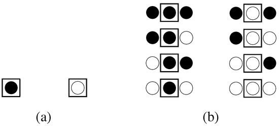
Figure 1. All possible discrete states of a single lattice site as subsystem of a linear lattice system when observed (a) isolated from its z nearest neighbors and (b) associated with its neighbors. In a linear lattice, considering only the nearest neighbors, $z=2$.

Figure 1. All possible discrete states of a single lattice site as subsystem of a linear lattice system when observed (a) isolated from its z nearest neighbors and (b) associated with its neighbors. In a linear lattice, considering only the nearest neighbors, $z=2$.

However, a concept of an isolated lattice which does not take its nearest, interacting neighbors into account does not allow for the formulation of constraints including interaction energies between sites, even though such constraints are essential for model development. For this reason, we introduce the concept of a single lattice site associated with its z nearest neighbors as subsystem, z representing the coordination number. The subsystem comprises ($z+1$) sites, as illustrated in Figure 1(b). In this concept, the discrete state of a lattice site is determined not only by its own molecule type but also by the type and arrangement of the z nearest neighbors contributing to energetic interactions. Here it is assumed that molecular interactions are confined to the nearest neighbors of the central molecule. If molecules beyond the direct neighbors also contribute to interactions, the concept of associated sites can be extended accordingly.

3.2.2. The unconstrained system

Shannon entropy of a subsystem: Without consideration of any constraints, it follows from equation (4a) that both of the two possible states shown in Figure 1(a) have the same probability, $p_{{\displaystyle ●}}=p_{{\displaystyle ○}}=\frac{1}{2}$, corresponding to a system with an equal number of black and white sites. Equation (4b) for an isolated site with 2 possible states yields

$$H_{\mathrm{s,iso}}=ln2$$

(51)

For an associated site shown in Figure 1(b), consisting of ($z+1$) sites, again according to Equation (4a), all possible states are equally probable. The number of possible states is now $2^{z+1}$, yielding the maximum Shannon entropy of

$$H_{\mathrm{s,ass}}=ln{2}^{z+1}=(z+1)ln2,$$

(52)

which is the ($z+1$)-fold of the Shannon entropy of the isolated site given by (51).

In a next step, the possibility of expressing the Shannon entropy of a compound lattice system by the Shannon entropy of its constituting subsystems shall be examined.

Shannon entropy of a compound system: When distributing two types of molecules over a lattice comprising N sites, the number of possible states is given by $2^N$, yielding the maximum Shannon entropy of

$$H_c=ln{2}^N=Nln2=N{H}_{\mathrm{s,iso}},$$

(53)

which is the N-fold of the maximum Shannon entropy of an isolated site, cf. Equation (51). When considering associated sites as subsystems, where a subsystem consists of ($z+1$) sites, the number of subsystems is

$$\widehat{N}=\frac{N}{z+1}$$

Now the number of states of the compound system is ${2^{z+1}}^{\widehat{N}}$, and the according Shannon entropy yields

$$H_c=ln{2^{z+1}}^{\widehat{N}}=\widehat{N}ln{2}^{z+1}=\widehat{N}{H}_{\mathrm{s,ass}},$$

(54)

which is the $\widehat{N}$-fold of the maximum Shannon entropy of an associated site, cf. Equation (52).

Equations (52)-(54) reveal the homogeneity of the Shannon entropy of unconstrained lattice systems, cf. Equation (8):

$$H_c=N{H}_s,$$

where $H_c$ now denotes the Shannon entropy of the whole lattice as compound system, $H_s$ is the Shannon entropy of the considered subsystem, i.e., isolated or associated site, and N is the number of subsystems.

3.2.3. System considering constraints

There are basically three types of constraints to be considered in a lattice system: Energy, composition and the equivalence of contact pairs between molecules of different types.

Energy: As mentioned at the beginning of section 3.2, the intended purpose of lattice systems is the consideration of interaction energies between adjacent lattice sites. Therefore, the concept of a single lattice site associated with its nearest neighbors was introduced in section 3.2.1. to be used as subsystem. Based on this concept, constraints considering interaction energies can be formulated generically in the form

$$\langle u\rangle =\sum _{i=1}^m{u}_i{p}_i^{ass}$$

(55)

which is in line with (12), $u_i$ designating the energy assigned to the central molecule of an associated site, $p_i^{\mathrm{ass}}$ its probability of residing in state i and $\langle u\rangle$ the mean value of energy. Figure 2 illustrates this nomenclature.

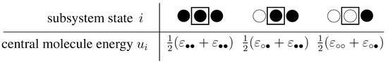
Figure 2. Examples for states and related energies of an associated lattice site as subsystem. ε denotes the interaction energy between two sites, where each site is assigned the half of it.

Figure 2. Examples for states and related energies of an associated lattice site as subsystem. ε denotes the interaction energy between two sites, where each site is assigned the half of it.

To formulate the energy assigned to a compound lattice consisting of N associated sites as subsystems, we use the index k to denote the state of the compound system which is determined by the states of its subsystems: $k\widehat{=}{i}_1,\dots ,i_N$. With this nomenclature, the energy of a compound system in state k is $U_k$, where

$$U_k=U_{i_1,\dots ,i_N}=u_{i_1}+\dots +u_{i_N},$$

which is analogous to (21). Recalling equations (22) to (25) for the mean values of energies, it follows that

$$\langle U\rangle =\langle u_1\rangle +\dots +\langle u_N\rangle$$

Because all single subsystems are of the same kind and no single subsystem is preferred to another, their mean value is the same, resulting in

$$\begin{array}{ccc}\hfill \langle u_1\rangle =\langle u_2\rangle =& \dots & =\langle u_N\rangle \equiv \langle u\rangle \hfill \end{array}$$

$$\begin{array}{ccc}\hfill \langle U\rangle & =& N\langle u\rangle ,\hfill \end{array}$$

(56)

which is analogous to (26). Using (56) as the only constraint aside from the normalization of probabilities, maximization of the Shannon entropy analog to (13) requires solution of the Lagrange function

$$\mathcal{L}=H_c-{\lambda }_1\langle U\rangle -{\lambda }_2\sum _i\left\{p_i\right\}\stackrel{!}{=}max.$$

(57)

Application of the maximization principle to (57) in line with (27) - (34) finally results in

$$H_c=N{H}_{\mathrm{s,ass}}$$

(58)

as Shannon entropy of the compound lattice system, analogously to Equation (36). Equation (58) reveals that the Shannon entropy of a constrained lattice system can also be expressed through the Shannon entropy of subsystems, whereupon subsystems are single lattice sites associated with their respective nearest neighbors. As shown in section 2.4, several functions with the generic form of equation (55) can also be considered as constraints in the maximization principle.

Composition: In the simplest case of a binary system, there are molecules of two types constituting the lattice. The constraint for the compound system is simply $N_1=N{x}_1$, the total number of 1-molecules. $x_1$ can be interpreted in two ways: as relative fraction of 1-molecules in the system, or as probability to find a 1-molecule at a given site. Hence, if we consider compound systems of identical composition, $N_1$ behaves according to Equation (49), fulfilling the prerequisites for constraints that enable homogeneity of Shannon entropy. The same holds for $x_2$ which is related to $x_1$ by the normalization condition. This can easily be extended to systems comprising an arbitrary number of components.

Equivalence of contact pairs: Contact pairs designate the number of contacts between molecules of different types in the system, e.g. $N_{2-1}$ (read ’2 around 1’) the number of all 2-molecules around all molecules of type 1, and $N_{1-2}$ the number of all 1-molecules around all molecules of type 2. As the number of contacts between molecules of different types must not depend on the viewpoint, the equivalence $N_{2-1}=N_{1-2}$ has to be fulfilled in lattice systems generally, independent of the respective size. The according constraint for the maximization prinziple is

$$N_{2-1}-N_{1-2}=0$$

This equating to zero is a homogeneous function in terms of Equation (49).

In summary, all three types of constraints are homogeneous in terms of Equation (49), ensuring that after maximization the Shannon entropy of a compound system is also homogeneous. The complete Lagrange function finally comprises the mean values of energy, composition and equivalence of contact pairs as constraints to be considered in a lattice model. Practical application will be shown in a subsequent paper.

4. Conclusions

The scope of this paper was to clarify prerequisites for applying the concept of Shannon entropy and maximum entropy principle to thermodynamic modeling of extensive systems. The main criterion for applicability of this kind of modeling is the additivity of the Shannon entropy. It was shown that this additivity is guaranteed, provided that the additivity of the constraints is given. If a thermodynamic model comprises additive constraints, this prerequisite is fulfilled, and the method is explicitly applicable to systems of interacting components, i.e., real fluids. This was shown for two limiting cases of fluid phases, the ideal gas model and condensed phase lattice systems.

The main benefit of thermodynamic modeling based on Shannon entropy is that it makes the equilibrium distribution of discrete states available. This establishes new possibilities for thermodynamic and mass transport models as it allows consideration of a more detailed picture of physical behavior of matter on a molecular basis, beyond the scope of traditional modeling methods. This will be exploited in subsequent papers.

References

- Shannon, C.E. A Mathematical Theory of Communication. Bell Sys. Techn. Journ. 1948, 27, 379–423,623–656. [Google Scholar] [CrossRef]
- Jaynes, E.T. Information Theory and Statistical Mechanics. Phys. Rev. 1957, 106, 620–630. [Google Scholar] [CrossRef]
- Jaynes, E.T. Information Theory and Statistical Mechanics. II. Phys. Rev. 1957, 108, 171–189. [Google Scholar] [CrossRef]
- Jaynes, E.T. Gibbs vs Boltzmann Entropies. Am. Journ. Phys. 1965, 33, 391–398. [Google Scholar] [CrossRef]
- Wehrl, A. General Properties of Entropy. Rev. Mod. Phys. 1978, 50, 221–260. [Google Scholar] [CrossRef]
- Guiasu, S.; Shenitzer, A. The Principle of Maximum Entropy. Math. Intell. 1985, 7, 42–48. [Google Scholar] [CrossRef]
- Ben-Naim, A. Entropy Demystified; World Scientific Publishing: Singapore, 2008. [Google Scholar]
- Ben-Naim, A. A Farewell to Entropy: Statistical Thermodynamics Based in Information; World Scientific Publishing: Singapore, 2008. [Google Scholar]
- Curado, E.; Tsallis, C. Generalized Statistical Mechanics: Connection with Thermodynamics. J. Phys. A 1991, 24, L69–L72. [Google Scholar] [CrossRef]
- Tsallis, C. Nonadditive Entropy: The Concept and its Use. Europ. Phys. Journ. A 2009, 40, 257–266. [Google Scholar] [CrossRef]
- Maczek, A. Statistical Thermodynamics; Oxford University Press: Oxford, UK, 1998. [Google Scholar]
- Wilde, D.J.; Beightler, C.S. Foundations of Optimization; Prentice-Hall: Englewood Cliffs, NJ, USA, 1967. [Google Scholar]
- Fowler, R.H.; Kapitza, P.; Mott, N.F.; Bullard, E.C. Mixtures - The Theory of the Equilibrium Properties of Some Simple Classes of Mixtures, Solutions and Alloys; Oxford at the Clarendon Press, 1952. [Google Scholar]
- Abrams, D.S.; Prausnitz, J.M. Statistical Thermodynamics of Liquid Mixtures: A New Expression for the Excess Gibbs Energy of Partly or Completely Miscible Systems. AIChE J. 1975, 21, 116–128. [Google Scholar] [CrossRef]
- Bronneberg, R.; Pfennig, A. MOQUAC, a New Expression for the Excess Gibbs Energy based on Molecular Orientations. Fluid Phase Equilib. 2013, 338, 67–77. [Google Scholar] [CrossRef]
© 2014 by the authors; licensee MDPI, Basel, Switzerland. This article is an open access article distributed under the terms and conditions of the Creative Commons Attribution license ( http://creativecommons.org/licenses/by/3.0/).