Simulation of Entropy Generation under Stall Conditions in a Centrifugal Fan

Abstract

Rotating stalls are generally the first instability met in turbomachinery, before surges. This 3D phenomenon is characterized by one or more stalled flow cells which rotate at a fraction of the impeller speed. The goal of the present work is to shed some light on the entropy generation in a centrifugal fan under rotating stall conditions. A numerical simulation of entropy generation is carried out with the ANSYS Fluent software which solves the Navier-Stokes equations and user defined function (UDF). The entropy generation characteristics in the centrifugal fan for five typical conditions are presented and discussed, involving the design condition, conditions on occurrence and development of stall inception, the rotating stall conditions with two throttle coefficients. The results show that the entropy generation increases after the occurrence of stall inception. The high entropy generation areas move along the circumferential and axial directions, and finally merge into one stall cell. The entropy generation rate during circumferential propagation of the stall cell is also discussed, showing that the entropy generation history is similar to sine curves in impeller and volute, and the volute tongue has a great influence on entropy generation in the centrifugal fan.

1. Introduction

Nowadays, fans are used extensively in the chemical industry, thermal power plants and so on. Rotating stalls which occur for small flow rates are a common instability phenomenon. This instability is responsible for the reduction of performance and large vibrations. When rotating stalls occur, a complex three-dimensional phenomenon involving the separation of boundary layer, vortex generation and secondary flow formation [1] becomes more obvious. The turbulent dissipation of the fan increases and the performance decreases.

Entropy generation is a good indicator of the energy loss and irreversibility of the system. Analysis of the entropy generation characteristics could help engineers to find out the zones for which energy is lost. This would contribute to the energy savings and optimization of the fan. It also helps understanding the mechanism of stalls from the energy point of view. Nowadays, the entropy theory is widely used in the heat transfer field. Bejan [2,3] studied the decrease of available energy and the increase of entropy generation in the heat transfer process. Herpe [4] analyzed the entropy prodution rate due to the viscous disspation and heat transfer in a finned oval tube. Hassan [5] presented theoretical research on entropy generation variation due to heat transfer and flow in nanofluid suspensions. Recently, researchers have mainly focused on the mechanism and active control of stalls. Experimental and numerical methods are two ways to study the rotating stall phenomenon. Ohta [6] studied the post-stall characteristics of surges and rotating stalls with experiments in an axial flow compressor. He discovered an active control method that succeeded in an expansion of the stable operational region of the compressor. Wang [7] carried out an experimental study on a G4-73 No.8D centrifugal fan by using harmonic wavelets. The study found that the stall point is close to the maximum efficiency point on the fan performance curve and the stall indication should get more attention. Meanwhile, some researchers have worked on the details of the flow field during stalls based on numerical simulations. Gourdain [8,9] numerically studied the rotating stall in a subsonic compressor, and discovered that stall cells are caused by the upstream flow disorganization and rotating stalls are initiated by an up-stream modal wave. Choi [10] found that the mis-staggered blade is instrumental to stall initiation because the increasing blade loading intensified the tip leakage flow to cause spillage around the leading edge of the trailing blade. Wang [11] analyzed that the reason for rotating stalls occurring at the suction side of the blade is the decrease of flow rate in a centrifugal fan. Nie [12] elucidated the relevance of early stall inception and the unsteady tip leakage vortex and proposed a tip air injection control system. Wu [13] studied the formation of the tip secondary vortex and the periodic flow phenomena in near-tip passages of a transonic compressor rotor in near stall conditions. Moghaddam [14] presented a numerical simulation to control rotating stalls and surges in jet engine compression systems by using a controller. Lucius [15] evaluated the risk of resonance by analyzing the stall frequency during rotating stalls in a centrifugal pump.

This paper numerically studies the entropy generation in a centrifugal fan under stall conditions. To achieve this aim, the present work focuses on two aspects: simulation of the rotating stall phenomenon in a back-inclined centrifugal fan and analysis of the entropy generation characteristics at different stall stages. In Section 2, the numerical method with the model studied and the particular boundary conditions used is presented. In Section 3, the simulation results are discussed. The simulation results under the design conditions are firstly validated by comparing them with the experimental data. Then, the entropy generation characteristics from stall inception to the rotating stall condition are investigated. Finally, the entropy generation rate during circumferential propagation of the stall cell are discussed.

2. Numerical Model

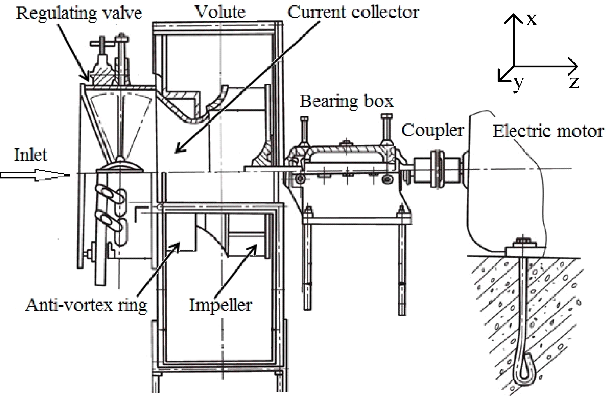
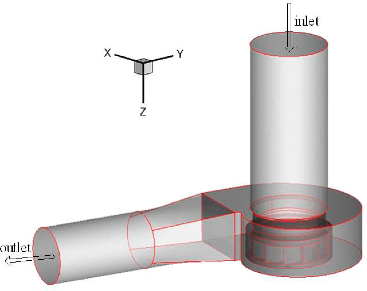
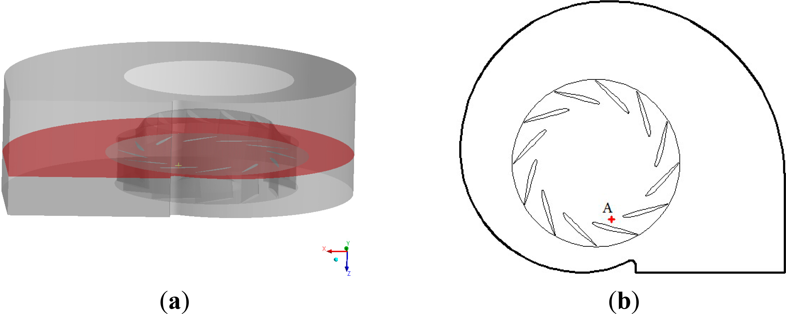
2.1. Geometry Model

The G4-73 back-inclined centrifugal fan was selected as the research object. As shown in Figure 1, the main parts of the system include impeller, volute, current collector and anti-vortex. The key parameters of the fan are listed in

Table 1. Key parameters of the centrifugal fan.

Parameter	Value
Inlet diameter of impeller D (cm)	56.8
Outlet width of impeller H (cm)	80
Number of blades Zb	12
Exit stagger angle β (deg)	45
Rotation speed (r/min)	1450

. The computational grid is established with the Gambit software, as shown in Figure 2. Two pipes of 2.6 m length are connected to the inlet and outlet of the fan, respectively, in order to minimize the influence of reflection.

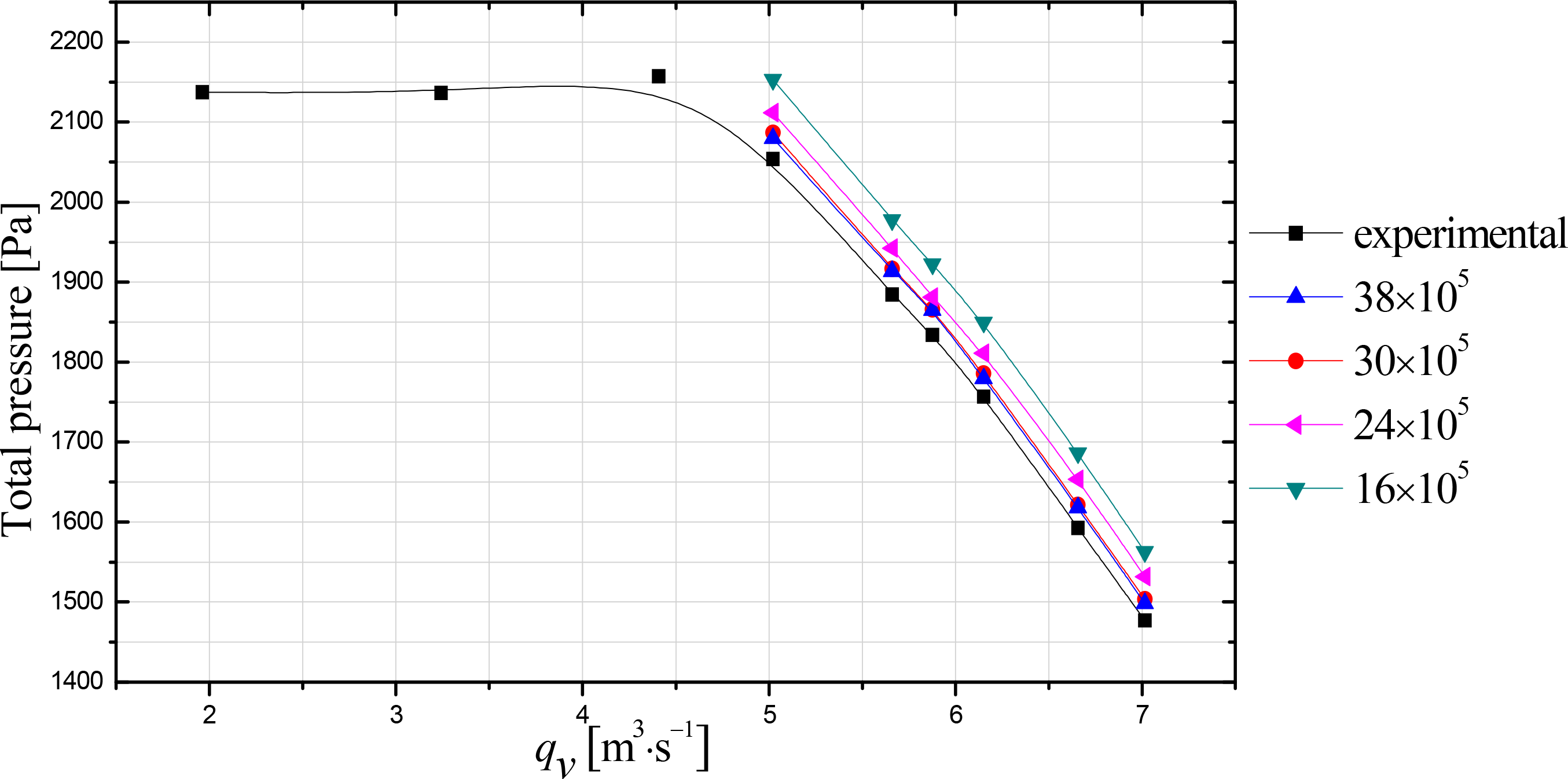
2.2. Throttle Model

Classical boundary conditions at the outlet of the fan, such as uniform static pressure, cannot be utilized efficiently to simulate the flow field near the operating point with maximum static pressure. When the slope of the static pressure curve becomes very small, the convergence of the solver slows down. Therefore, an idealized throttle function is applied at the outlet of the fan. The static pressure at the outlet is determined by a quadratic law [9]:

$$p_{s_{\mathit{out}}}\left(t\right)=p_{i_{\mathit{in}}}+\frac{k_0}{2k_1}\rho U^2$$

(1)

The advantage of this method lies in its ability to capture the transient outlet static pressure and avoid numerical instabilities when the mass flow is reduced. It has a better capacity to capture physical flow features when the rotating stall is studied. The position of the operating point is set only by means of the throttle coefficient k₁.

2.3. Governing Equations

The fluid temperature is fairly constant in the centrifugal fan, so fluid properties are assumed to be constant. The flow field in the fan is governed with unsteady Navier-Stokes equations. The Realizable k−ε model is selected as the turbulence model and an enhanced wall function is employed in the near wall region. The governing equations, including the continuity equation, the momentum equation and the realizable k−ε equations, are shown as Equations (2)–(5):

$$\frac{\partial v_i}{\partial x_i}=0$$

(2)

$$\rho \frac{\partial v_i}{\partial t}+\rho \frac{\partial }{\partial x_j}\left(v_i{v}_j\right)=-\frac{\partial p}{\partial x_i}+\frac{\partial }{\partial x_j}\left(\mu \frac{\partial v_i}{\partial x_j}-\rho \overline{v_i^{\prime }{v}_j^{\prime }}\right)+\rho f_i$$

(3)

$$\frac{dk}{dt}=\frac{\partial }{\partial x_j}\left[\left(\mu +\frac{C_{\mu }\left(k^2/\epsilon \right)}{{\sigma }_k}\right)\frac{\partial k}{\partial x_j}\right]+G_k-\epsilon$$

(4)

$$\frac{d\epsilon }{dt}=\frac{\partial }{\partial x_j}\left[\left(\mu +\frac{C_{\mu }\left(k^2/\epsilon \right)}{{\sigma }_{\epsilon }}\right)\frac{\partial \epsilon }{\partial x_j}\right]-C_{1\epsilon }\frac{\epsilon }{k}{G}_k-C_{2\epsilon }\frac{{\epsilon }^2}{k}$$

(5)

Among them,C_1ε = 1.44, C_2ε = 1.92, C_μ = 0.09, σ_k = 1.0, σ_ε = 1.3.

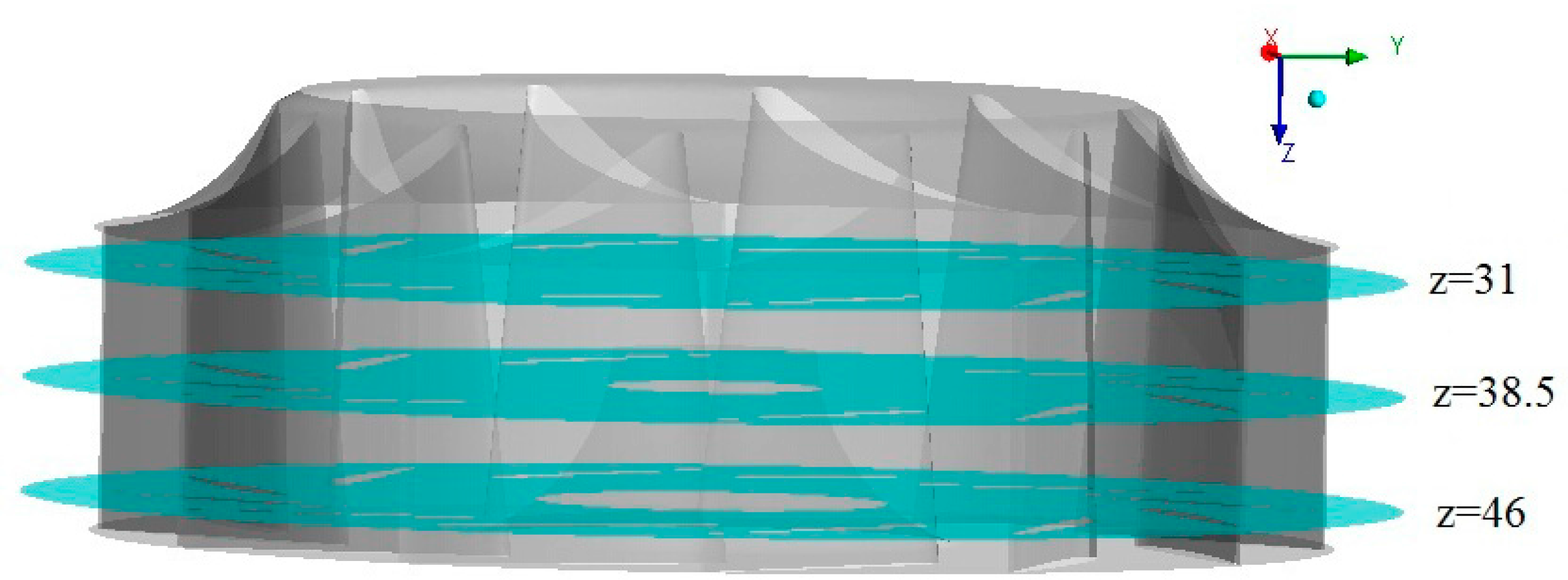
2.4. Meshing Strategy

The quality of the mesh has an important effect on the accuracy of the solution. An unstructured mesh is used in the impeller and volute with refinement around the volute tongue and blades. The size function is used to refine the mesh in some key regions such as the impeller and the volute to improve the calculation accuracy. A hexahedral structured grid is used in other parts of the fan. The multiple reference frames (MRF) model was applied in steady calculation and the moving mesh model in unsteady simulation. Boundary layer meshes are attached to the blade surfaces and the volute wall to ensure that the distance between the wall and the first layer grid nodes in the range of y⁺ < 1.

The resolution of the mesh has been tested to ensure that the calculated results are grid-independent. The number of cells was varied as 16 × 10⁵, 24 × 10⁵, 30 × 10⁵, 38 × 10⁵ and 60 × 10⁵, respectively. As shown in Figure 3, the error between the numerical and the experimental results [16] decreases with the grid resolution. As a compromise between accuracy and computational effort, the grid size is selected as 30 × 10⁵. At different mass flow rates (as shown in Figure 3), the error is within 3% and the numerical results show good agreement with the experimental results.

2.5. Entropy Generation Calculation

The entropy generation includes two terms: entropy generation by dissipation and entropy generation by heat transfer. Since the temperature is constant in this paper, the entropy generation due to heat transfer is neglected.

The entropy generation in the fan is closely related to the so-called turbulent dissipation rate Φ̅ which appears in the k−ε equation. The entropy generation inside the centrifugal fan includes two parts: entropy generation due to viscous dissipation S_D and entropy generation due to turbulent dissipation S_D′. The local entropy generation per unit volume of the fan is calculated using the following equations:

$$\overline{\Phi }/T=S_D+S_{D^{\prime }}$$

(6)

$$S_D=\mu /\overline{T}\{2\left[{\left(\frac{\partial {\upsilon }_x}{\partial x}\right)}^2+{\left(\frac{\partial {\upsilon }_y}{\partial y}\right)}^2+{\left(\frac{\partial {\upsilon }_z}{\partial z}\right)}^2\right]+{\left(\frac{\partial {\upsilon }_x}{\partial y}+\frac{\partial {\upsilon }_y}{\partial x}\right)}^2+{\left(\frac{\partial {\upsilon }_x}{\partial z}+\frac{\partial {\upsilon }_z}{\partial x}\right)}^2+{\left(\frac{\partial {\upsilon }_y}{\partial z}+\frac{\partial {\upsilon }_z}{\partial y}\right)}^2\}$$

(7)

$$S_{D^{\prime }}=\frac{\mu }{\overline{T}}\{2\left[\overline{{\left(\frac{\partial {\upsilon }_x^{\prime }}{\partial x}\right)}^2}+\overline{{\left(\frac{\partial {\upsilon }_y^{\prime }}{\partial y}\right)}^2}+\overline{{\left(\frac{\partial {\upsilon }_z^{\prime }}{\partial z}\right)}^2}\right]+\overline{{\left(\frac{\partial {\upsilon }_x^{\prime }}{\partial y}+\frac{\partial {\upsilon }_y^{\prime }}{\partial x}\right)}^2}+\overline{{\left(\frac{\partial {\upsilon }_x^{\prime }}{\partial z}+\frac{\partial {\upsilon }_z^{\prime }}{\partial x}\right)}^2}+\overline{{\left(\frac{\partial {\upsilon }_y}{\partial z}+\frac{\partial {\upsilon }_z^{\prime }}{\partial y}\right)}^2}\}$$

(8)

Equation (7), containing the mean velocity gradients, can be interpreted as entropy production by dissipation in the mean flow field. It is referred to the direct dissipation. Equation (8), containing the gradients of the fluctuating velocities hence is the entropy production by dissipation in the fluctuating part of the flow field. It is referred to the indirect dissipation. The fluctuating velocity in Equation (6) cannot be obtained directly from the numerical solution. Kock [17] proposed an assumption that S_D′ is related to the turbulent dissipation rate and temperature. Thus, S_D′ is calculated as follows:

$$S_{D^{\prime }}=\rho \epsilon /\overline{T}$$

(9)

3. Results and Discussion

The monitoring point “A” is set inside the impeller on the z = 34.44 cm cross-section. The location of the monitoring point “A” is marked in Figure 4. Time is in shaft revolutions. The curve of relative velocity at point A varying with revolution is shown in Figure 5.

It can be seen that the amplitude of the fluctuation of relative velocity increases after the 175th revolution until stall inception occurs. It takes 50 further revolutions from stall inception to establish a stall cell in the impeller. During this transition period, the amplitude of the fluctuation of relative velocity is growing gradually.

For the frequency domain analysis of the relative velocity during the stall process, the relative velocity signal registered by a fixed probe at point A is transformed with a Fast Fourier Transform. The power spectrum is shown in Figure 6. It can be seen that the stall frequency of the fan is 14.15 Hz. The experimental result of the stall frequency is 14.4 Hz [18]. Thus, the simulation result is consistent with the experimental result, and the correctness of the simulation result is validated.

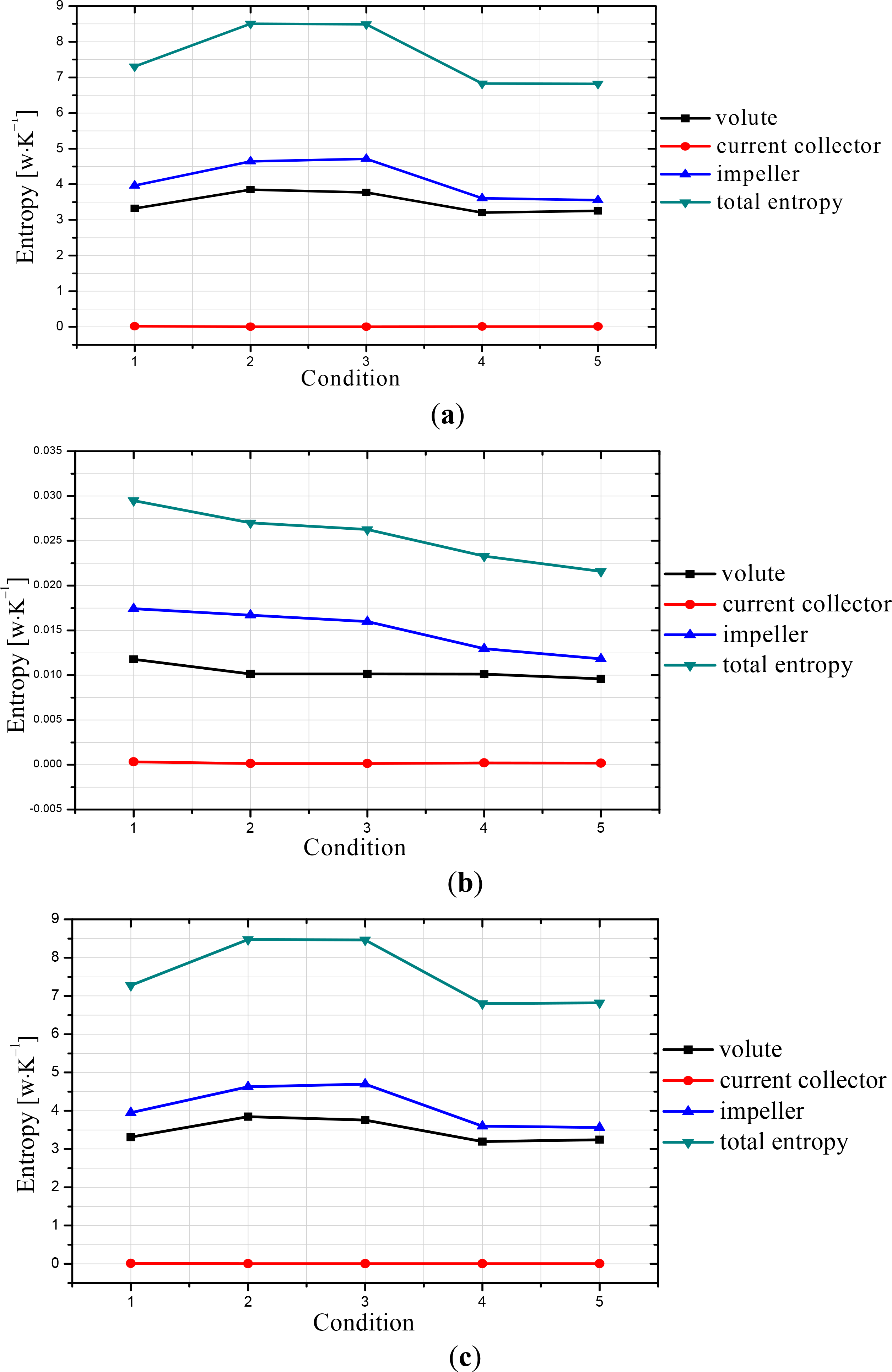
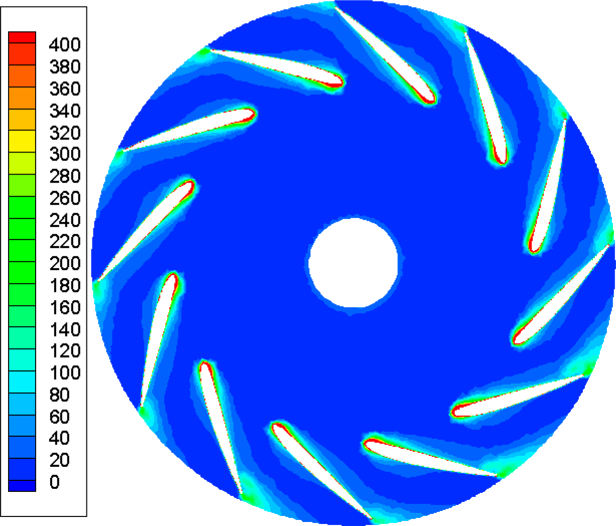
3.1. Entropy Generation Characteristics on Five Typical Conditions

In order to investigate the entropy generation characteristics before and after the occurrence of stall, five typical conditions are selected. The information is shown in

Table 2. The information of the five typical conditions.

Number	Condition	Remark
1	k1=2	Close to the design condition.
2	k1 = 0.89 (the 150th revolution)	The throttle coefficient is 0.89. The stall hasn’t occurred.
3	k1 = 0.89 (the 185th revolution)	The throttle coefficient is 0.89. The stall inception has occurred.
4	k1 = 0.89 (the 240th revolution)	The throttle coefficient is 0.89. The stall cell is established in impeller.
5	k1 = 0.7	The throttle coefficient is 0.7. The flow rate is smaller the condition 4. The stall cell is established in the impeller.

.

The entropy generation in the centrifugal fan is shown in Figure 7. It can be seen that entropy generation is concentrated in the impeller and volute. The flow structure inside the impeller and volute is complex, and separation of the boundary layer and secondary flow formation is observed. Meanwhile, the entropy generation in the current collector is very small and may be ignored. As shown in the diagram, the fluctuation of the entropy generation in impeller is obvious, so the stall has a great influence on the entropy generation in the impeller. The total entropy generations on the 2nd condition and 3rd condition are higher for the evolutionary process of the stall cell, while, the entropy generation on the 4th condition and 5th condition is reduced gradually. Since the velocity tends to stable values after the stall cell is mature, the entropy generation decreases in the passages which are far away from the stall cell.

Comparing Figure 8b with Figure 8c, the entropy generation caused by viscous dissipation is very small and it is two orders of magnitude lower than the entropy generation caused by turbulence dissipation. Therefore, the energy loss of the fan mainly comes from the turbulent dissipation, while the viscous dissipation can nearly be ignored.

3.2. Entropy Generation Characteristics on Design Condition

The entropy generation contour for the design conditions is shown in Figure 8. From the figure, it is clear that distribution of entropy generation in each impeller passage is almost the same. Due to the incidence loss in the front disc, the boundary layer separation at the surface of the blades and the wake turbulent jet at the outlet of the impeller, there are 12 high entropy generation areas, respectively, at the leading edge and trailing edge of the blades. However, the entropy generation in the impeller passages is small.

3.3. Entropy Generation Characteristics on Stall Inception Condition

When the valve opening k₁ is 0.89, the entropy generation characteristics at different sections of the impeller in the 150th revolution (the stall inception hasn’t occurred) are shown in Figure 10. The z = 31 cm section is near the front disc, z = 38.5 cm section is in the middle cross section of the impeller, and z = 46 cm section is close to the rear disk. The location of the three sections is shown in Figure 9. As shown in Figure 10a, there are 12 high entropy generation areas at the inlet of the impeller. The entropy generation at the outlet of the impeller is high, especially in the region near the volute tongue. Comparing Figure 10b with Figure 10a, the high entropy generation areas of the inlet impeller move towards the outlet and reach the middle of the channels. As shown in Figure 10c, the high entropy generation areas almost disappear. This is because the axial flow turns into radial flow at the inlet of the impeller, the relative velocity on z = 31 cm section is small, while the incidence angle is big, leading to the separation of boundary layer and vortex formation. Therefore, the entropy generation is high on the z = 31 cm section. The incidence angle decreases along the z axis, so the entropy generation decreases along the axial section. Meanwhile, the vortex is big near the volute tongue and the influence of the volute tongue on the entropy generation is significant.

In Figure 10b, the high entropy generation areas become larger compared with Figure 9. With the decrease of flow rate, the incidence angle increase and the size of separated vortex becomes bigger, so the energy loss becomes larger. Meanwhile, the entropy generation increases significantly near the volute tongue because the jet-wake gets enhanced and the velocity gradient increases. As the result, the entropy generation of the impeller increases obviously because of the vortex energy loss and the irregular structure of the volute tongue.

Figure 11 shows the contours of entropy generation on the three cross sections mentioned above in the 185th revolution. The distribution of the entropy generation is non-uniform on z = 31 cm section. There are two high entropy generation areas and one of them is near the volute tongue.

On the z = 38.5 cm section, there are also two high entropy generation areas. Since the incidence angle is smaller than that of z = 31 cm section, the entropy generation is smaller. Compared with the design conditions, the entropy generation increases significantly and the high entropy generation areas move along the axial and radial directions. After the stall inception occurs, the turbulent fluctuation increases, so the energy loss increases as well. In the 185th revolution, the stall cells move to z = 38.5 cm section, while the flow near the rear disk hasn’t been affected yet. In summary, the entropy generation decreases along the axial direction, and the entropy generation near the front disc is higher than that near the rear disk. The entropy generation increases and the number of high entropy generation areas turn into two during the process from the 1st condition to the 3rd condition.

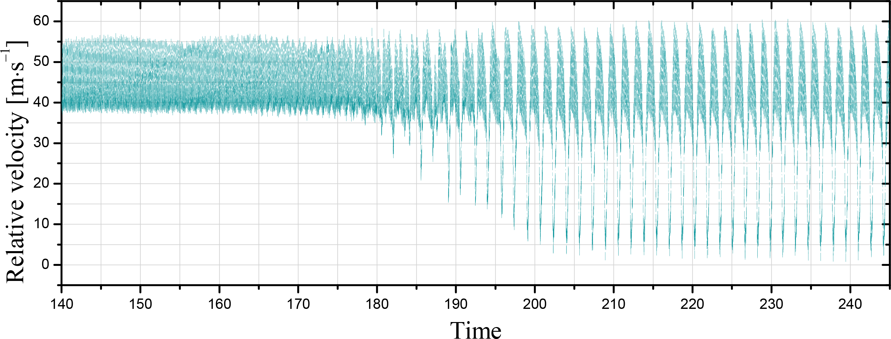
3.4. Entropy Generation Characteristics during Rotating Stall Conditions

In the 240th revolution, the stall cell is already mature. The entropy generation on the three axial sections is shown in Figure 12. One high entropy generation area occupying three passages is observed on the three sections. Compared with Figure 11, the high entropy generation areas move towards the outlet of the impeller along the radial direction. The number of the high entropy generation area turns into one and the full-span stall occurs.

When the valve opening turns to 0.7, the contours of entropy generation during deep rotating stall are shown in Figure 13. One smaller high entropy generation area is observed at three different sections, respectively, compared with Figure 12. Because of the effects of the stall cells and volute tongue, the high entropy generation area is stretched and scattered. As shown Figure 13c, a high entropy generation area is noticed and the stall cells move to the z = 46 cm section along the axial direction.

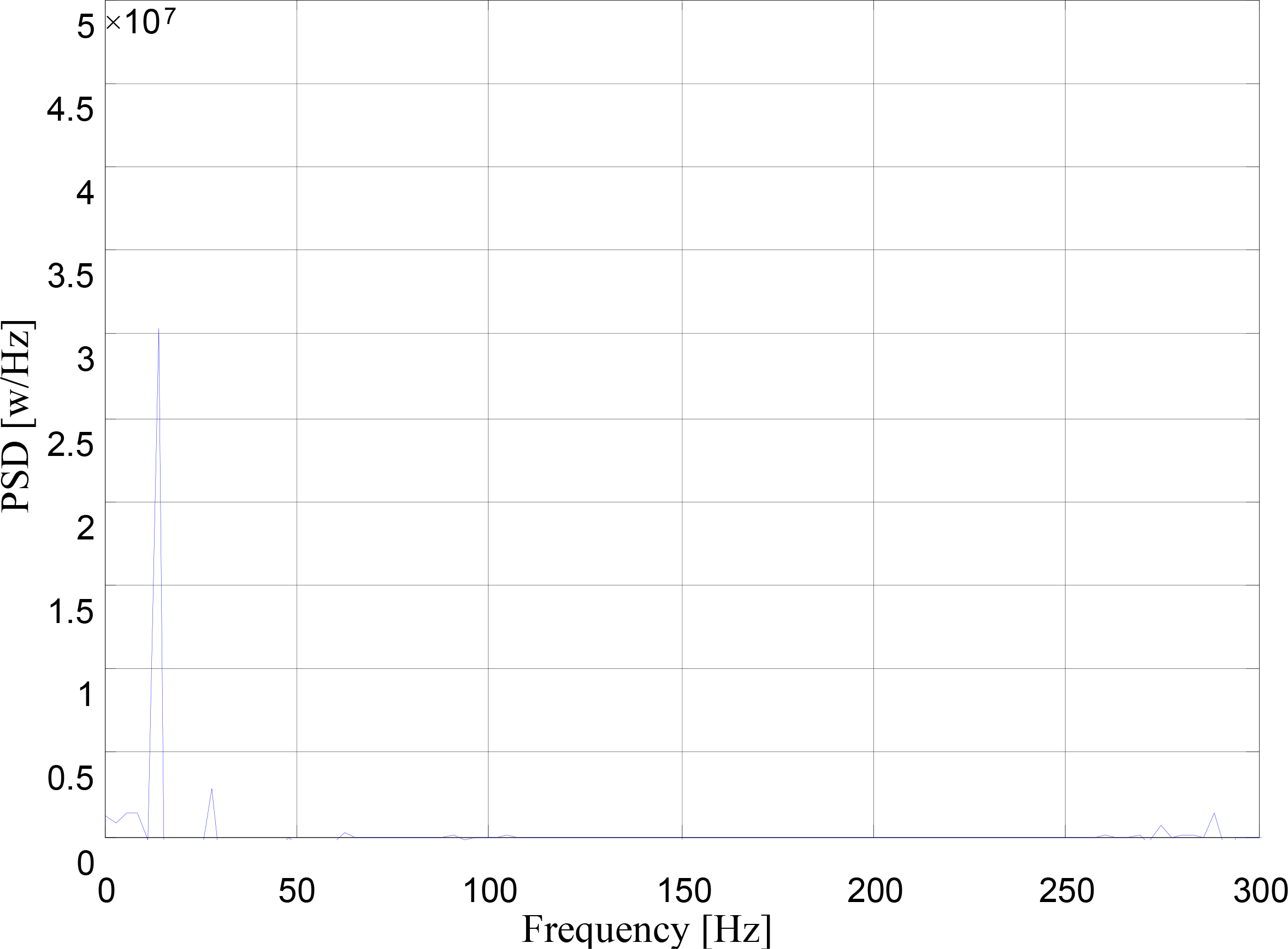
3.5. Entropy Generation Characteristics During the Circumference Propagation of Stall Cell

Taking a twelfth of a revolution as a period, the entropy generation on design condition from the 123rd revolution to the 127th is illustrated in Figure 14. It can be seen that the fluctuation of the entropy generation is inconspicuous. The entropy generation in the impeller is larger than that in the volute.

When the valve opening k₁ is 0.89, the fluctuation of entropy generation from 250th revolution to 254th revolution is shown in Figure 15. The entropy generation curves of the impeller and that of volute are both similar to sine. The fluctuation cycle is 1.625 revolutions. That is the stall cell rotates along the circumferential direction at 61.5% speed of the impeller. The stall cell moves more slowly than impeller, so the propagation direction of the stall cells is opposite to the rotation direction of the impeller in the relative coordinate system.

The average entropy generation of the impeller is 3.866 w·K⁻¹, and the amplitude is 0.338 w·K⁻¹. The average entropy generation of the volute is 2.959 w·K⁻¹, and the amplitude is 0.254 w·K⁻¹. The oscillation periods of entropy generation in the impeller and volute are the same, but there is a phase shift of a half period. For the “A” condition the entropy generation of the impeller comes to its minimum, the entropy generation of volute reaches its peak. However the fluctuation of the total entropy generation, which is the superposition of the two, is smaller.

The contours of entropy generation for the “A” and “B” conditions are shown in Figure 16, respectively. As shown in Figure 16a, a high entropy generation area is noticed near the volute tongue. The volute tongue has great influence on the entropy generation. The high entropy generation area occupies three passages in the impeller. The entropy generation is less in the passages which are far away from the stall cell, so the entropy generation inside the volute is very small except a small area near the volute tongue. Therefore, the entropy generation of the impeller comes to its maximum, while the entropy generation of volute reaches its minimum value. Figure 16b shows the contour of entropy generation with the minimum entropy generation of the impeller and the maximum of the volute. During the rotation of the impeller, the stall cells move away from the volute tongue gradually, so does the high entropy generation area. As the effect of the stall cells and volute tongue becomes weak, high entropy generation area becomes smaller in the impeller and the high entropy generation area is stretched leading to the increase of entropy generation in the volute.

Figure 17 displays the fluctuation of entropy generation from the 286th revolution to 290th when the valve opening is 0.7. The waveform of the curves is similar to that when k₁ = 0.89. With the decrease of flow rate, the stall cell has greater influence on the entropy generation and the amplitude of the curve is larger. The average entropy generation of the impeller is 3.877 w·K⁻¹, and the amplitude is 0.452 w·K⁻¹. The average entropy generation of the volute is 2.941 w·K⁻¹, and the amplitude is 0.325 w·K⁻¹. The fluctuation cycle is 1.6 revolutions which is same to the period on the k₁ = 0.89 condition. The contours of entropy generation on A’ and B’ condition are shown in Figure 18 respectively. The contour of entropy generation corresponding to the extreme value of entropy generation in impeller and volute are the same to k₁ = 0.89 condition. In other words, after the maturation of the stall cell, the propagation velocity of the stall cell remains the same even if the flow rate changes.

4. Conclusions

A back-inclined centrifugal fan has been simulated numerically to study the entropy generation characteristics. The main results are summarized as follows:

(1)

The entropy generation is concentrated on the impeller and volute for boundary layer separation, turbulence, secondary flow formation, etc. The turbulent dissipation is more significant than viscous dissipation on the entropy generation. With the decrease of the flow rate, the entropy generation becomes larger due to the increase of the incidence angle.

(2)

At the stall inception stage, the high entropy generation areas become larger compared to the design condition. There are two high entropy areas and one of them is near the volute tongue. During the maturation of stall cell stage, the number of high entropy generation areas turn into one and the entropy generation is less in the passages away from stall cell. The high entropy generation areas move along the circumferential and axial directions.

(3)

During the circumferential propagation of stall cell, the volute tongue has great influence on entropy generation. The entropy generation curves of the impeller and that of volute are similar to sine curves, and their oscillation periods are both 1.6 revolutions. With the decrease of flow rate, the stall cell has greater influence on entropy generation and the amplitude of the curves become larger.

References

- An, L.S. The structure and performance of fan. In Pumps and Fans; China Electric Power Press: Beijing, China, 2001; pp. 31–36. (in Chinese) [Google Scholar]
- Bejan, A. Entropy minimization: The new thermodynamics of finite-size devices and finite-time processes. Appl. Phys 1996, 79, 1191–1218. [Google Scholar]
- Makinde, O.D.; Chinyoka, T.; Adetayo, S. Numerical investigation of entropy generation in an unsteady flow through a porous pipe with suction. Exergy 2013, 12, 279–297. [Google Scholar]
- Herpe, J.; Bougeard, D.; Russeil, S.; Stanciu, M. Numerical investigation of local entropy production rate of a finned oval tube with vortex generators. Int. J. Thermal Sci 2009, 48, 922–935. [Google Scholar]
- Hassan, M.; Sadri, R.; Ahmadi, G.; Dahari, M.B.; Kazi, S.N.; Safaei, M.R.; Sadeghinezhad, E. Numerical study of entropy generation in a flowing nanofluid used in micro- and minichannels. Entropy 2013, 15, 144–155. [Google Scholar]
- Ohta, Y.; Fujita, Y.; Morita, D. Unsteady Behavior of Surge and Rotating Stall in an Axial Flow Compressor. J. Therm. Sci 2012, 21, 302–310. [Google Scholar]
- Wang, S.L.; Hou, J.H.; An, L.S.; Ai, J.C. Experiment study and feature extraction on rotating stall of centrifugal fan in power plant. Compress. Blower Fan Tech 2003, 6, 15–19. (in Chinese). [Google Scholar]
- Gourdain, N.; Burguburu, S.; Leboeuf, S.; Miton, H. Numerical simulation of rotating stall in a subsonic compressor. Aerosp. Sci. Tech 2006, 10, 9–18. [Google Scholar]
- Gourdain, N.; Burguburu, S.; Leboeuf, S.; Michon, G.J. Simulation of Rotating Stall in a Whole Stage of an Axial Compressor. Comput. Fluid 2010, 39, 1644–1655. [Google Scholar]
- Choi, M.; Vahdati, M.; Imregun, M. Effects of Fan Speed on Rotating Stall Inception and Recovery. J. Turbomach 2011, 133, 041013. [Google Scholar]
- Zhang, L.; Wang, S.L.; Zhang, Q.; Wu, Z.R. Fluid dynamics characteristics of rotating stall in a centrifugal fan. Proc. CSEE 2012, 32, 95–101. (in Chinese). [Google Scholar]
- Li, J.C.; Tong, Z.T.; Lin, F.; Nie, C.Q. Experimental investigation of tip air injection base on detection mechanism of early stall warning. J. Eng. Thermophys 2012, 33, 573–577. (in Chinese). [Google Scholar]
- Wu, Y.H.; Zhao, K.; Tian, J.T.; Chu, W.L. Analysis of near-tip unsteady flow field in a transonic compressor rotor at near stall condition. J. Eng. Thermophys 2012, 33, 401–404. (in Chinese). [Google Scholar]
- Moghaddam, J.J.; Farahani, M.H.; Amanifard, N. A neural network-based sliding-mode control for rotating stall and surge in axial compressors. Appl. Soft Comput 2011, 11, 1036–1043. [Google Scholar]
- Lucius, A.; Brenner, G. Numerical Simulation and Evaluation of Velocity Fluctuations During Rotating Stall of a Centrifugal Pump. J. Fluids Eng 2011, 133, 081102. [Google Scholar]
- Zhang, L.; Wang, S.; Hu, C.; Zhang, Q. Multi-objective optimization design and experimental investigation of centrifugal fan performance. Chin. J. Mech. Eng 2013, 26, 1267–1276. [Google Scholar]
- Kock, F.; Herwig, H. Local Entropy Production in Turbulent Shear Flows: A High-Reynolds Number Model with Wall Functions. Heat Mass Transf 2004, 47, 2205–2215. [Google Scholar]
- Zhang, L.; Liang, S.; Hu, C. Flow and noise characteristics of centrifugal fan under different stall conditions. Math. Probl. Eng 2014, 2014, 403541. [Google Scholar]