A Note of Caution on Maximizing Entropy

1
Department of Preventive Medicine, Northwestern University Feinberg School of Medicine, Chicago, IL 60611, USA
2
Department of Biomedical Informatics, University of Pittsburgh, Pittsburgh, PA 15232, USA
*
Author to whom correspondence should be addressed.
Entropy 2014, 16(7), 4004-4014; https://doi.org/10.3390/e16074004
Submission received: 4 May 2014
/
Revised: 10 July 2014
/
Accepted: 15 July 2014
/
Published: 17 July 2014
(This article belongs to the Special Issue Maximum Entropy and Its Application)
Abstract
:The Principle of Maximum Entropy is often used to update probabilities due to evidence instead of performing Bayesian updating using Bayes’ Theorem, and its use often has efficacious results. However, in some circumstances the results seem unacceptable and unintuitive. This paper discusses some of these cases, and discusses how to identify some of the situations in which this principle should not be used. The paper starts by reviewing three approaches to probability, namely the classical approach, the limiting frequency approach, and the Bayesian approach. It then introduces maximum entropy and shows its relationship to the three approaches. Next, through examples, it shows that maximizing entropy sometimes can stand in direct opposition to Bayesian updating based on reasonable prior beliefs. The paper concludes that if we take the Bayesian approach that probability is about reasonable belief based on all available information, then we can resolve the conflict between the maximum entropy approach and the Bayesian approach that is demonstrated in the examples.
1. Introduction
The Principle of Maximum Entropy is often used to update probabilities due to evidence instead of performing Bayesian updating using Bayes’ Theorem, and its use often has efficacious results. However, in some circumstances the results seem unacceptable and unintuitive. This paper discusses some of these, and discusses how to identify some of the situations in which this principle should not be used. First, we provide a brief discussion of the three major approaches to probability in order to provide background and context. See [1] for a more complete introduction.
The classical approach to probability refers to most efforts to deal with probability up to and including the time of Laplace (1749–1827). Laplace and his contemporaries did not consider their efforts an “approach”; it is a term applied retrospectively. At its heart we find Laplace’s definition of probability [2]:
The theory of chance consists in reducing all the events of some kind to a certain number of cases equally possible, that is to say, such as we may be equally undecided about in regard to their existence, and in determining the number of cases favorable to the event whose probability is sought. The ratio of this number to that of all the cases possible is the measure of the probability.
Probabilities are assigned within the framework of the classical approach by using the principle of indifference (a term first used by J.M. Keynes in 1921 [3]). The fundamental idea is that “alternatives are always to be judged equiprobable if we have no reason to expect or prefer one over the other” [4]. Classical examples of applying the principle of indifference include assigning 1/2 to the probability of heads in a coin toss, and assigning 1/52 to the probability of each card in an ordinary deck of 52 cards. Many paradoxes have been developed concerning applications of the principle of indifference. Neapolitan [1] discusses some of them.
Laplace and his contemporaries believed in determinism, as is evident from the following statement [2]:
We ought then to regard the present state of the universe as the effect of its anterior state and as the cause of the one which is to follow. Given for one instant an intelligence which could comprehend all the forces by which nature is animated and the respective situation of the beings who compose it—an intelligence sufficiently vast to submit these data to analysis—it would embrace in the same formula the movements of the greatest bodies of the universe and those of the lightest atom; for it, nothing would be uncertain and the future, as the past, would be present to its eyes.
Suppose now that we assign P(heads) = 0.5 in the case of a coin toss, and we toss the coin 1000 times. How many times would we expect heads to occur? Today, most of us would say about 500. This notion of probability as a relative frequency of the occurrence of an event was formalized in the early 20th century by Richard von Mises (although he had 19th century precursors such as Cournot and Venn). Specifically, if an experiment is repeated n times and Sn(E) is the number of times an event E occurs, then von Mises [5] defined the probability of E as follows:
This is called the limiting frequency approach to probability. The argument is that if, for example, we tossed a coin 1000 times, it might turn up head 543 times, after 10,000 tosses there might be 5067 heads, and after 100,000 tosses 50,085 heads. The point is that as the number of repetitions of the experiment increases, the number of stable digits in the relative frequency increases. Therefore, according to the theory, there is a limiting value and that value is the probability. Of course, this cannot be established empirically since we can never proceed indefinitely; however, von Mises [5] said that this approach is applicable whenever we have “sufficient reason to believe that the relative frequency of the observed attribute would tend to a fixed limit if the observations were indefinitely continued.” In 1946 Kerrich [6] conducted many experiments concerning games of chance such as throwing a die. He found that the relative frequency did seem to converge and it converged to the value obtained using the principle of indifference.
Inherent in the von Mises theory is that separate trials of experiment are independent. That is, suppose P(heads) = 0.5, and we repeatedly toss the coin 11 times. Then regardless of whether we observe 10 straight heads, 10 straight tails, or some mixture of the two, P(heads) is still 0.5 on the 11th toss. That is, the relative frequency of heads on the 11th toss in the limit is 0.5 for all the different combinations of occurrences on the first 10 tosses. In 1971 Iverson et al. [7] conducted experiments substantiating that this is the case.
In a sense, the limiting frequency approach subsumes the classical approach because in practice probabilities obtained with the principle of indifference are about equal to the observed relative frequencies. However, it allows us to apply probability theory to a much broader domain. For example, suppose we are repeatedly tossing a thumbtack, and when it lands on its flat head we say “heads” while when it lasts with the point and top touching we say “tails”. Due to the asymmetry of the thumbtack we would not apply the principle of indifference and say P(heads) = 0.5. However, we can toss the thumbtack 10,000 times and if it lands heads 6673 times, we can approximate P(heads) by 0.6673. Most applications of probability in statistics concern relative frequencies that cannot be obtained using the principle of indifference. For example, if we do a randomly controlled experiment where we give 1000 individuals medication X for hair regrowth and give 1000 individuals placebo, and investigated the fractions of individuals that regrow hair, we are estimating assumed objective probabilities (infinite relative frequencies) by the observed relative frequencies.
Both of the approaches just presented assume, in some sense, that objective probabilities exist. The classical approach assumes a probability is logically correct based on the information, while the limiting frequency approach assumes a probability is a physical property of nature.
Suppose now that we are considering betting on the football game between the Chicago Bears and the Detroit Lions. To ascertain a fair bet, gambler Joe needs to assess the probability of the Bears winning. If he would be willing to give up $6 if the Bears lose for the promise to receive $4 if they win, then for Joe P(BearsWin) = 0.6. If Mary would be willing to give up $7 if they lose for the promise to receive $3 if they win then for Mary P(BearsWin) = 0.7. This is called the subjective or Bayesian approach to probability. This approach also evolved largely in the 20th century, and is discussed at length in [8,9]. According to this approach, objective probabilities do not always exist; however we can ordinarily assign a probability that is a property of an individual’s belief. There are many versions of “Bayesians,” some of which deny the existence of objective probabilities. Good [10] states there are 46,656 varieties of Bayesians. Versions include subjective, personalist, objective, empirical Bayes (EB), semi-EB, semi-Bayes, epistemic, intuitionist, logical, fuzzy, hierarchical, pseudo, quasi, compound, parametric, nonparametric, hyperparametric, and non-hyperparametric Bayes. In a sense, the Bayesian approach subsumes the relative frequency approach in the following way. First, it allows us to apply probability to events such as the Bears/Lions football game. Since this game will only be played once, the limiting frequency approach, which requires a repeatable experiment, is not applicable. There are many important applications of probability that involve such events, not the least of which is economic forecasting. Second, suppose we have a repeatable experiment such as a coin toss. Then we say the sequence that represents the outcome of a number of repetitions of the experiment is exchangeable for an individual, if all sequences that are the same length and have the same number of occurrences of heads are assigned the same probability by the individual. That is, if we let 0 represent “tails” and 1 represent “heads”, the sequences 1000100100 and 1110000000 are assigned the same probability. Furthermore, any other sequence containing three heads and seven tails has that same probability. The assumption of exchangeability in the subjective approach is analogous to the assumption of independence in the relative frequency approach. As Zabell [11] discusses, if we assume exchangeability then, except for the case of very strong prior beliefs (e.g. the individual says she knows the probability of heads for certain and no number of repetitions of the experiment will affect her belief) than after the experiment is repeated n times the individual’s P(heads) must be about equal to the relative frequency of heads when n is large.
2. The Principle of Maximum Entropy
One interpretation of the principle of indifference is that there is an experiment which uses some physical process to randomly obtain exactly one of the alternatives, and that this process treats all of the alternatives equitably. Another interpretation is that we should apply it whenever the information gives us no reason to choose one alternative over the other. This interpretation assume that it is not necessary that there is a physical process that treats all the alternatives equitably; rather it is only necessary that there is nothing in the information to imply that they are not treated equitably. Jaynes [12] is a proponent of this interpretation. According to Jaynes, assigning values equitably in such a case is the least presumptive assignment of probabilities. Based on this idea, Jaynes developed an extension to the principle of indifference called the principle of maximum entropy. Before describing this principle, we note that Jaynes does not call probabilities, obtained with the principle of maximum entropy, “objective” in the sense of the relative frequency approach. However he does state [12]:
andBut it is just the point of the maximum-entropy principle that it achieves “objectivity” of our inferences in the sense that we base our predictions only on the information that we do, in fact, have...
The probabilities .... are an entirely correct description of our state of knowledge...
Therefore, it seems that Jaynes’ approach does consider probabilities objective in the sense of the logical approaches of Keynes [3] and Carnap [13]. That is, he feels that there are logically correct probabilities based on the information.
Jaynes extends the principle of indifference as follows: If there is information about the experiment which implies that the probabilities cannot all be 1/n, then the least presumptuous assignment of probabilities is the one which comes as close as possible to distributing the probabilities equitably while satisfying the information. Jaynes calls this rule for assigning probabilities the principle of maximum entropy. If we define the entropy H in the experiment by:
where pi is the probability of the ith alternative, then it can be shown that H is minimized when pi = 1 for some i, and maximized when pi = 1/n for all i. The principle of maximum entropy states that in the light of information which implies that the probabilities cannot all be 1/n, the least presumptuous assignment of probabilities is the one which maximizes H.
Jaynes illustrates the principle with his Brandeis dice problem. He supposes a six-sided die for which it is known, in repeated rolls, that the average number of spots is 4.5, not 3.5, as would be expected for a fair die. That is:
Given this information and nothing else, the problem is to determine the probabilities of the six sides turning up on the next role. According to the principle of maximum entropy, the solution is the one that maximizes H relative to the mean value constraint. Jaynes solves the problem as a standard variational problem using the Lagrange multiplier technique. He determines the probabilities to be:
Jaynes [12] offers cogent evidence justifying the principle of maximum entropy. In particular, he shows that the principle predicts results in physics that agree with our macroscopic measurements. Jaynes [12] notes:
The price is that we must loosen the connections between probability and frequency, by returning to the original viewpoint of Bernoulli and Laplace. The only new feature is that their Principle of Insufficient Reason is now generalized to the Principle of Maximum Entropy. Once this is accepted, the general formalism of statistical mechanics...can be derived in a few lines without wasting a minute on ergodic theory...The price we have paid for this simplification is that we cannot interpret the canonical distribution as giving the frequencies with which a system goes into the various states. But nobody has ever needed that interpretation anyway. In recognizing that the canonical distribution represents only our state of knowledge when we have certain partial information derived from macroscopic measurements, we are not losing anything we had before.
So, Jaynes is able to substantiate the existence of probabilities using the principle of maximum entropy with evidence which is not relative frequencies, dismissing, in the case of these applications to physics, Nagel’s [14] criticism of the classical approach, which was that there is no proof that the probabilities obtained using the principle of indifference will agree with relative frequencies.
3. Difficulties with the Principle of Maximum Entropy
When Jaynes extends the principle of maximum entropy from applications to physics to problems such as the Brandeis dice problem, the physical evidence for the probabilities no longer exists, and we need some other evidence if we are to claim the principle achieves “objectivity of our inferences....” [12].
Jaynes’ does provide a justification for maximizing entropy in the case of the Brandeis dice problem. However, the justification is relative to the interpretation that the mean value constraint is determined from repeated throws of the die. Jaynes [12] states the following:
When a die is tossed, the number of spots up can have any value i in 1≤i≤6. Suppose a die has been tossed N times and we are told only that the average number of spots was not 3.5 as we would expect from an “honest” die but 4.5. Given this information and nothing else, what probability should we assign to i spots in the next toss?
Jaynes [15] then shows that if the mean value is obtained by measuring the outcomes of N repeated tosses and exchangeability is assumed, then the maximum entropy probability assignments are consistent with achieving the constraint in exponentially more ways than any other assignment of probabilities. So, with this interpretation of the mean value constraint, he provides a persuasive argument justifying the use of maximum entropy to assign probabilities.
Before proceeding, we provide a concrete example. Suppose we have a three-sided die (We illustrate the problem with a die for the sake of focus. However, our discussion applies to any experiment with three outcomes.) with 1, 2, and 3 spots inscribed on the respective sides, and the only information about the die is that the average number of spots in repeated rolls is known to be 2, the value that would be obtained if the die were fair. For example, perhaps the die was purchased at a novelty store, and so we have no reason to believe that it is fair or that it has a particular bias. However, a friend later tossed the die many times and found that the mean value is 2. The friend shared the mean value with us, but not the actual results of the individual rolls. So, we believe almost for certain that the mean values is 2, and this is our only information about the probabilities. Since values of 1/3 for all pi satisfy the mean value constraint, and since these values yield the absolute maximum entropy, the maximum entropy solution is easily seen to be pi = 1/3 for all i.
Next we investigate another way to perhaps achieve “objectivity of inferences” in the case of the example just presented. Since we have no reason to believe the die is fair, we could consider all probability distributions that satisfy the constraints in the problem equally probable. That is, we apply the principle of indifference to the probability values themselves. To that end, if we assume pi has some objective value, and if we let xi be a random variable representing the possible values that pi could have, then the constraints in the problem are as follows:
If we fix x1 and solve for x2 and x3 we obtain:
Since 0≤x2≤1, the only values of x1 that are possible are ones satisfying the inequality:
So, the possible values of x1 are all values in the interval [0, 0.5], and it is clear each of these values can occur in exactly one way; that is, with x3 = x1 and x2 = 1 − 2x1. Therefore, based on an application of the principle of indifference, the probability density function for p1 having value x1 in the interval [0,0.5] is the uniform density function 1/(0.5–0) = 2, and the expected value of x1 is given by:
In the same way, if we fix x2, we find that each value of x2 in the interval [0,1] can occur in exactly and that the expected value of x2, obtained using the principle of indifference, is 0.5. Finally, fixing x3, we find that each value of x3 in the interval [0,0.5] can occur in exactly one way and no other values can occur, and therefore the expected value of x3, obtained using the principle of indifference, is 0.25.
This solution is clearly different from the maximum entropy solution of 1/3 for all pi. It is also intuitively appealing, since, given that p2 could be as high as 1, while the other probabilities are bound above by 0.5, we may be inclined to bet on 2. Once the information gives us reason to prefer one alternative over the others, it is troublesome to claim that the probabilities, based on the information, are equal.
Next, let’s investigate the Bayesian solution to obtaining the conditional probabilities given that the mean value of 2 for the three-sided die is obtained from N tosses of the die (Jaynes’ interpretation), and see how that solution compares to the maximum entropy solution and to our solution obtained by applying the principle of indifference to the probabilities.
First, we provide further background. Suppose we have a repeatable experiment with a discrete number of outcomes such as the tossing of the three-sided die. Zabell [16] shows that if we make certain reasonable assumptions about an individual’s beliefs concerning the probabilities of the outcomes of the experiment, then that individuals beliefs about those probabilities must be represented by a Dirichlet distribution of the probability values. The Dirichlet density function with parameters a1, a2,..., ak,
, where a1, a2,..., ak are real numbers > 0, is:
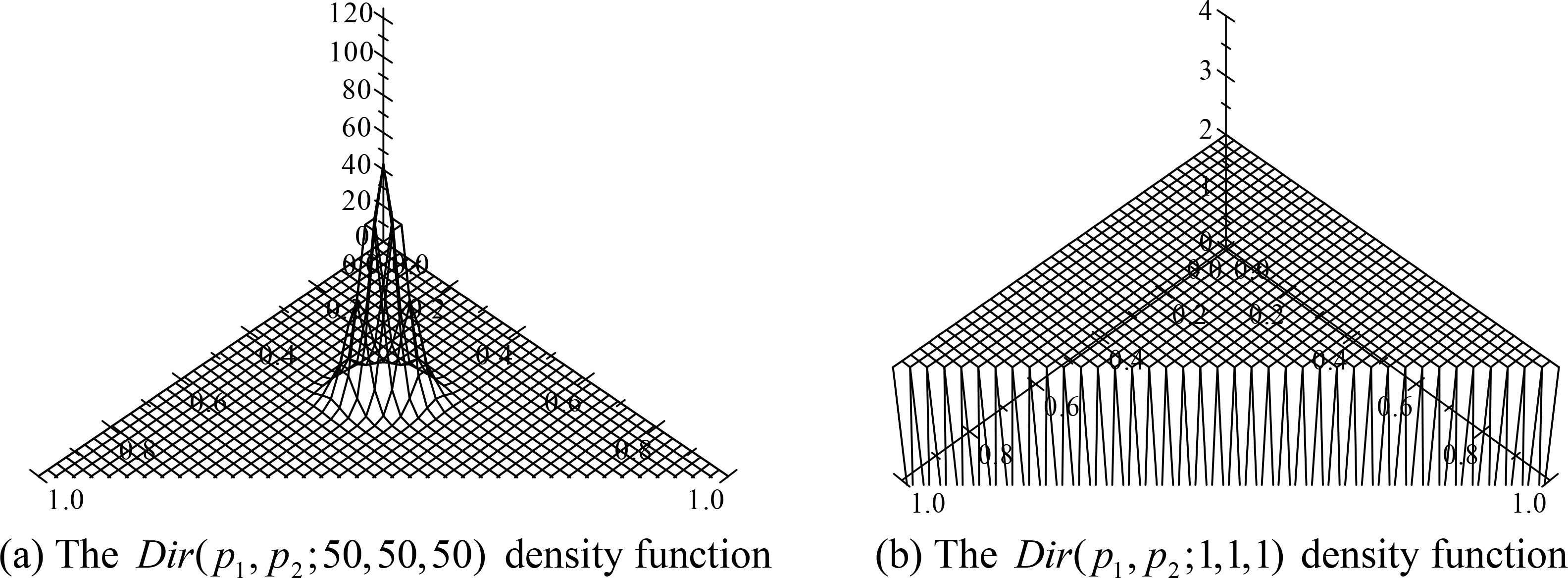
The Dirichlet density function is denoted by Dir(p1, p2,...pk−1; a1, a2,..., ak). When we use this density function to represent our prior belief about a probability that is a relative frequency, intuitively the parameter ai represents the number of times our experience is equivalent to having seen alternative i occur ai times. For example, in the case of a normal six-sided die bought from a store that sells reputable gambling apparatus, we might feel very strongly that all alternatives have the same probability and take a1 = a2 = ⋯ = a6 = 50 because our prior experience is equivalent to having seen each alternative occur 50 times. In the case of a three-sided die bought at a novelty store, we may have no reason to prefer one outcome over the other, but we would not feel strongly that they all have the same probability. So we might take a1 = a2 = a3 = 1. Figure 1a shows the Dir(p1, p2;50,50,50) density function and Figure 1b shows the Dir(p1, p2;1,1,1). Note that the Dir(p1, p2;50,50,50) is highly peaked at the point (1/3,1/3). The reason is that we have strong belief the die is fair. Note further that Dir(p1, p2;1,1,1) is uniform over the entire allowable range of values. The reason is that we are completely ignorant as to the probability of each outcome.
Suppose we represent our prior belief about the probabilities of the outcomes of the three-sided die with the Dir(p1, p2; a1, a2, a3), observe s1 occurrences of 1, s2 occurrences of 2, and s3 occurrences of the 3, and assume infinite exchangeability. Then it is possible to show [1,17] that the updated conditional probabilities based on these observations are given by:
where M = a1 + a2 + a3 and N = s1 + s2 + s3.
Assume our belief about the probabilities of the three alternatives is represented by the Dirichlet density function Dir(p1, p2; a1, a2, a3). Let MVN = r represent the event that the sample average equals r in the first N rolls, and let p(2| MVN = r) be the probability of a 2 on the N + 1 st role given MVN = r. If MVN = 2, it is not hard to see that we must have s1 = s3. If we assume all possible values of s1 and s2 that satisfy this constraint are equally probable given MVN = 2 and that N is even, then according to Equation 1 the probability of 2 on the N + 1 st role is given by
It is straightforward that:
We obtain a similar result for N odd. Hence the solution, which was obtained by applying the principle of indifference to the probability values subject to the mean value constraint, agrees with the solution obtained by representing our belief about the probabilities using the Dir(p1, p2; a1, a2, a3) density function, assuming all outcomes that satisfy the mean value constraint are equally probable, and doing Bayesian updating.
So, the maximum entropy solution does not agree with the Bayesian solution if we consider all outcomes satisfying the mean value constraint equally probable. We would need to make some other assumption about the likelihood of these outcomes to make Bayesian updating consistent with the maximum entropy solution. In some particular application perhaps there may be a justification for choosing a non-uniform distribution on the outcomes. However, in the absence of any other information, it seems least presumptuous to make it uniform.
Herein lies the conflict between maximizing entropy and using the Bayesian solution we provided. Is it least presumptuous to keep the probabilities of the outcomes of the toss as close to uniform as possible (maximum entropy solution), or is it least presumptuous to put a uniform distribution on all outcomes of the N tosses that satisfy the mean value constraint?
4. Conclusions
In general, there is no answer to the question just posed. Rather a way out of this conundrum is to carefully analyze each situation and adopt the strategy that seems most applicable, as suggested by Seidenfield [18]:
A pragmatic appeal to successful applications of the MAXENT formalism cannot be dismissed lightly. The objections that I raise in this paper are general. Whether (and if so, how) the researchers who apply MAXENT avoid these difficulties remains an open question. Perhaps, by appealing to extra, discipline-specific assumptions they find ways to resolve conflicts with MAXENT theory. A case-by-case examination is called for.
For example, consider again the case of the three-side die. If one purchased the die at a store which is known to sell fair gambling apparatus, then a priori one would believe almost for certain that the die was very close to fair, and so maximizing entropy relative to a mean value constraint could be regarded as a reasonable source of subjective probabilities. On the other hand, in the case where one had no reason to believe a priori that the die was fair (the die was purchased at a novelty store), the application of the principle of indifference, as done above, seems to be a more reasonable source of subjective probabilities. Notice that in both these situations we are conditioning on more information that just the mean value constraint. They represent different cases.
5. Further Reading
Dias and Shimony [19] forwarded criticisms of the principle of maximum entropy similar to those presented here. Jaynes [20] responds to these criticisms. Uffink [21,22] provides more detailed mathematical arguments making points similar to the ones forwarded here. Diaconis and Zabell [23] show that there are a number of distance measures that one could use to update probability. You then find the nearest probability to the one you start out with, but which incorporates the new constraint. They note that these different measures can give quite different answers and there is no natural way to choose between them.
Acknowledgments
This work was supported by National Library of Medicine grants number R00LM010822 and R01LM011663. We would like to thank Sandy Zabell for discussing the arguments in the manuscript with us, and for reading the entire draft of the manuscript and suggesting many useful modifications.
Author Contributions
Conceived the idea to write a manuscript concerning difficulties with maximizing entropy: Richard E. Neapolitan. Conceived the arguments in the manuscript: Richard E. Neapolitan, Xia Jiang. Discussed the content at length: Richard E. Neapolitan, Xia Jiang. Wrote the first draft of the manuscript: Richard E. Neapolitan. Contributed to the writing of the manuscript: Xia Jiang. Reviewed the final draft of the manuscript and made corrections/modifications: Richard E. Neapolitan, Xia Jiang. Both authors have read and approved the final manuscript.
Conflicts of Interest
The authors declare no conflict of interest.
References
- Neapolitan, R.E. Probabilistic Reasoning in Expert Systems; Wiley: New York, NY, USA, 1989. [Google Scholar]
- De Laplace, P.S. Philosophical Essay on Probabilities; Springer: New York, NY, USA, 1995. [Google Scholar]
- Keynes, J.M. A Treatise on Probability; Dover: New York, NY, USA, 2004. [Google Scholar]
- Weatherford, R. Philosophical Foundations of Probability Theory; Routledge & Kegan Paul: London, UK, 1982. [Google Scholar]
- Von Mises, R. Probability, Statistics, and Truth; George Allen & Unwin: London, UK, 1957. [Google Scholar]
- Kerrich, J.M. An Experimental Introduction to the Theory of Probability; Einer Munskgaard: Copenhagen, Denmark, 1946. [Google Scholar]
- Iverson, G.R.; Longcor, W.H.; Mosteller, F.; Gilbert, J.P.; Youtz, C. Bias and Runs in Dice Throwing and Recording: A Few Million Throws. Psychometrika 1971, 36, 417–434. [Google Scholar]
- De Finetti, B. Probability, Induction, and Statistics; Wiley: New York, NY, USA, 1972. [Google Scholar]
- Good, I.J. The Estimation of Probabilities: An Essay on Modern Bayesian Methods; Research Monograph No. 30; MIT Press: Cambridge, MA, USA, 1965. [Google Scholar]
- Good, I.J. 46656 Varieties of Bayesianism. Am. Stat 1971, 25, 62–63. [Google Scholar]
- Zabell, S.L. Symmetry and Its Discontents. In Causation, Chance, and Credence; Skyrms, B., Harper, W.L., Eds.; Kluwer Academics: Dordrecht, The Netherlands, 1988. [Google Scholar]
- Jaynes, E.T. Where Do We Stand on Maximum Entropy? In The Maximum Entropy Formalism; Levine, R.D., Tribus, M., Eds.; MIT Press: Cambridge, MA, USA, 1979. [Google Scholar]
- Carnap, R. Logical Foundations of Probability; University of Chicago Press: Chicago, IL, USA, 1950. [Google Scholar]
- Nagel, E. Principles of the Theory of Probability; University of Chicago Press: Chicago, IL, USA, 1939. [Google Scholar]
- Jaynes, E.T. On the Rationale of Maximum-Entropy Methods. Proc. IEEE 1982, 70, 939–952. [Google Scholar]
- Zabell, S.L. W.E. Johnson’s “Sufficientness” Postulate. Ann. Stat 1982, 10, 1090–1099. [Google Scholar]
- Neapolitan, R.E. Learning Bayesian Networks; Prentice Hall: Upper Saddle River, NJ, USA, 2004. [Google Scholar]
- Seidenfield, T. Entropy and Uncertainty. Philos. Sci 1986, 53, 259–287. [Google Scholar]
- Dias, P.M.C.; Shimony, A. . A Critique of Jaynes’ Maximum Entropy Principle. Adv. Appl. Math 1981, 2, 172–211. [Google Scholar]
- Jaynes, E.T. Some Random Observations. Synthese 1985, 63, 115–138. [Google Scholar]
- Uffink, J. Can the Maximum Entropy Principle be Explained as a Consistency Requirement? Stud. Hist. Philos. Sci. B Stud. Hist. Philos. Mod. Phys 1995, 26, 223–261. [Google Scholar]
- Uffink, J. The Constraint Rule of the Maximum Entropy Principle. Stud. Hist. Philos. Sci. B Stud. Hist. Philos. Mod. Phys 1996, 27, 47–79. [Google Scholar]
- Diaconis, P.; Zabell, S. Updating Subjective Probability. J. Am. Stat. Assoc 1982, 77, 822–830. [Google Scholar]
Figure 1.
Two Dirichlet density functions.

© 2014 by the authors; licensee MDPI, Basel, Switzerland This article is an open access article distributed under the terms and conditions of the Creative Commons Attribution license (http://creativecommons.org/licenses/by/3.0/).
Share and Cite
MDPI and ACS Style
Neapolitan, R.E.; Jiang, X. A Note of Caution on Maximizing Entropy. Entropy 2014, 16, 4004-4014. https://doi.org/10.3390/e16074004
AMA Style
Neapolitan RE, Jiang X. A Note of Caution on Maximizing Entropy. Entropy. 2014; 16(7):4004-4014. https://doi.org/10.3390/e16074004
Chicago/Turabian StyleNeapolitan, Richard E., and Xia Jiang. 2014. "A Note of Caution on Maximizing Entropy" Entropy 16, no. 7: 4004-4014. https://doi.org/10.3390/e16074004