An Entropy-Based Upper Bound Methodology for Robust Predictive Multi-Mode RCPSP Schedules

Abstract

Projects are an important part of our activities and regardless of their magnitude, scheduling is at the very core of every project. In an ideal world makespan minimization, which is the most commonly sought objective, would give us an advantage. However, every time we execute a project we have to deal with uncertainty; part of it coming from known sources and part remaining unknown until it affects us. For this reason, it is much more practical to focus on making our schedules robust, capable of handling uncertainty, and even to determine a range in which the project could be completed. In this paper we focus on an approach to determine such a range for the Multi-mode Resource Constrained Project Scheduling Problem (MRCPSP), a widely researched, NP-complete problem, but without adding any subjective considerations to its estimation. We do this by using a concept well known in the domain of thermodynamics, entropy and a three-stage approach. First we use Artificial Bee Colony (ABC)—an effective and powerful meta-heuristic—to determine a schedule with minimized makespan which serves as a lower bound. The second stage defines buffer times and creates an upper bound makespan using an entropy function, with the advantage over other methods that it only considers elements which are inherent to the schedule itself and does not introduce any subjectivity to the buffer time generation. In the last stage, we use the ABC algorithm with an objective function that seeks to maximize robustness while staying within the makespan boundaries defined previously and in some cases even below the lower boundary. We evaluate our approach with two different benchmarks sets: when using the PSPLIB for the MRCPSP benchmark set, the computational results indicate that it is possible to generate robust schedules which generally result in an increase of less than 10% of the best known solutions while increasing the robustness in at least 20% for practically every benchmark set. And, in an attempt to solve larger instances with 50 or 100 activities, we also used the MRCPSP/max benchmark sets, where the increase of the makespan is approximately 35% with respect to the best known solutions at the same time as with a 20% increase in robustness.

1. Introduction

Projects are an important part of our activities and regardless of their magnitude, scheduling is at the very core of every project. One of the most commonly sought objectives when scheduling projects is completing them on the shortest possible time considering both urgency and resource availability; and even though we might be aware of some of the risks that could affect our planned (baseline) schedule, there will always be a certain degree of uncertainty that will remain unaccounted for.

A formal and commonly accepted definition for project is: “a temporary organization to which resources are assigned to undertake a unique, novel and transient endeavor managing the inherent uncertainty and need for integration in order to deliver beneficial objectives of change” [1–3]. From this definition we notice that uncertainty is given and if we want to successfully complete our project we need to manage it. In practice, a rather common way to manage uncertainty is by adding a buffer time that consists basically of a percentage of the total estimated duration. This is a fast and easy way to account for unforeseen events but it is entirely subjective as it depends almost exclusively on the experience or inexperience of the scheduler. Besides, the scheduler has already included his personal judgment when estimating each activity’s duration. Including a subjective buffer time could be dangerously over or even underestimate both the schedule’s duration and its budget.

In this paper we approach buffer time generation borrowing a term from the field of thermodynamics, entropy. Our methodology estimates an upper bound for a project’s makespan that depends exclusively on the activity’s estimated duration and the precedence requirements. After the upper bound is generated we use a quality based robustness measure to generate schedules with maximized robustness and with a makespan that is at most (but not necessarily) as high as the upper bound (entropy containing) schedule. By using the concept of entropy we eliminate the subjectivity in buffer time generation, and provide an equally convenient procedure to account for uncertainty. The remainder of this paper is outlined as follows: Section 2 provides some background regarding the project scheduling problem, the way in which uncertainty has been handled in project scheduling, and the concept of robustness in scheduling. Section 3 describes the algorithm and the 3-stage methodology to generate schedules with maximized robustness and an entropy-based upper bound. Section 4 reports the computational results of the methodology when compared to the PSPLIB and MRCPSP/max benchmark instances. Finally, Section 5 presents the conclusions and future research directions.

2. Literature Review

2.1. Resource Constrained Project Scheduling Problem

In general, a project consists of a set of tasks, governed by precedence relationships. Usually, the objective of interest is to complete the project in the shortest possible time while obeying the established precedence. Project scheduling is less difficult when only precedence relations constrain the task scheduling and can be easily solved using techniques like Critical Path Method (CPM) and Program Evaluation and Review Technique (PERT). However, in most real situations, executing a task requires resources, which are generally available in limited amounts and this makes the project scheduling problem very difficult to solve optimally. When resources are constrained and each task can be executed in only one way, the scheduling problem is known as the Resource Constrained Project Scheduling Problem (RCPSP). The RCPSP has been studied by many authors and is known to be NP-Hard [4].

However, a more realistic situation is that in which each task can be completed in one out of several possible alternatives. Each alternative preferably leads to a different duration, and potentially requires either different resources and/or amount of resources. This problem, known as the multi-mode resource-constrained project scheduling problem (MRCPSP), is a generalization of the RCPSP. Kolisch [5] proved the NP-hardness of the MRCPSP as a generalization of the RCPSP.

2.1.1. Multi-mode Resource Constrained Project Scheduling Problem

The main difference between the single and multi-mode RCPSP are the amount of modes or ways in which an activity can be executed. Elmaghraby [6] introduced the concept of mode, which resembles real life project management where each activity can be done in one out of several alternatives. Each mode is characterized by its own duration, and they depend on the amount of resources they consume. This means that the project manager or scheduler can choose (if the mode is feasible) the amount of resource he is willing to invest or sacrifice in order to comply with the established due date. Another characteristic is the inclusion of non-renewable resources, along with the renewable resources already taken into account in the single mode RCPSP. The non-renewable resources are those whose total amount is limited over the project duration and the exhausted amount cannot be replenished, such as capital budget. When non-renewable resources are present in the project the problem becomes NP-complete [7]. Please refer to Talbot [8] for the details on the mathematical formulation of the MRCPSP with all the constraints.

Due to its complexity MRCPSP includes time/resource and resource/resource trade-offs for all resources types. De Reyck et al. [9] introduced the discrete time/resource trade off problem (DTRTP), which exemplifies the case that activities can be performed with different amounts of resources, resulting in different possible durations. Pollack-Johnson and Liberatore [10] studied discrepancies in quality between activity modes of DTRTP. Ranjbar et al. [11] extended a generalization of DTRTP with multiple resource types (MDTRTP). Such problem involves each renewable resource with time/resource trade off.

More researches regarding MRCPSP in the last decades can be found on Özdamar et al. [12], Pesch [13], Hartmann [14], Jósefowska et al. [15], Alcaraz et al. [16], Bouleiman and Lecocq [17], and Jarboui et al. [18]. Nudtasomboon and Randhawa [19] allowed pre-emption of activities in a multi-mode RCPSP. Salewski et al. [20] and Drexl et al. [21] extended the MRCPSP by introducing mode identity constraints, in which there are some activities that should be performed in the same way, e.g., by allocating the same resources to them. Erenguc et al. [22] introduced the crashable modes, where the duration of a mode can be shortened at the expense of an additional cost. This is a special case of the mode concept and has been a rather common practice among project managers when the project is running behind schedule. Bellenguez and Néron [23] considered activities which require staff members with certain skill levels.

Zhu et al. [24] employed a multi-mode problem with generalized resource constraints. Varma et al. [25] considered a multi-mode problem without nonrenewable resources. Multi-mode problems with generalized precedence constraints have been considered by De Reyck and Herroelen [26], Drexl et al. [21], Heilmann [27,28], Nonobe and Ibaraki [29], Brucker and Knust [30], Calhoun et al. [31], Sabzehparvar and Seyed-Hosseini [32] and Barrios et al. [33].

Furthermore, examples of quality considerations in MRCPSP can be found in: Tareghian and Taheri [34] whom employed the mode concept to consider quality but, their objective is to maximize the quality while the project’s deadline and budget (non-renewable resource capacity) must be observed. Also, Li and Womer [35] employed the mode concept to take quality considerations into account and whose goal is to find the reliability of a node in the supply chain. Tiwari et al. [36] proposed a model in which an activity may be started in a mode that does not allow completing the activity at a required quality level. Processing in such a mode then has to be followed by a rework mode that completes the activity.

2.1.2. Objectives Solved

Throughout decades, researchers have proposed many ways to tackle the MRCPSP using models that optimize different objectives. The objectives or performance indicators for projects can be divided in two broad categories: time performance indicators and financial evaluation indicators. However, these models usually do not take into account managing uncertainty in the projects, and if any disruption occurs, these deterministic schedules do not consider the proper idle times to improve flexibility and robustness [37].

2.1.2.1. Time Performance Indicators

Even though the most researched objective in MRCPSP is the minimization of makespan [38], objectives based on lateness, tardiness, and earliness have also been closely studied. Lateness (L_j) is the deviation of an activity’s completion time (C_j) from a given due date (d_j), (C_j–d_j), either a positive or negative value. Tardiness can be simply defined as the positive values of lateness, including 0 (T_j= max{0, C_j–d_j}), while the earliness would be the range of the absolute value of the negative values of lateness up to 0 (E_j = max{0, d_j–C_j}).

Franck and Schwindt [39] mentioned an MRCPSP with the objective of minimizing the sum of the earliness and tardiness values. Vanhoucke et al. [40] discussed a just-in-time objective which is achieved by minimizing the weighted sum of all earliness and tardiness values. Neumann et al. [41] studied the minimization of the maximum lateness and of the weighted total tardiness. An alternative objective minimizes the maximum value of all earliness and tardiness values. Lorenzoni et al. [42] proposed a variant where earliness and tardiness are measured with respect to a given time window in which an activity should be carried out. Nudtasomboon and Randhawa [19], Kolisch [43], Viana and de Sousa [44], and Ballestín et al. [45], considered the minimization of the weighted tardiness, which generalizes the makespan objective.

Nudtasomboon and Randhawa [19] proposed to minimize the sum of all activity completion times, while Rom et al. [46] minimized the weighted sum of the completion times. Similarly, Nazareth et al. [47] suggested minimizing the mean flow time, which is the average of all activity completion times. Vanhoucke [48] defined a set of time windows for each activity carrying out an activity within one of its time windows is desired due to quality considerations. The objective function minimizes penalties that are caused by executing activities outside their time windows.

2.1.2.2. Financial Indicators

Maniezzo and Mingozzi [49] and Möhring et al. [50,51] considered costs for each activity dependent on the activity’s start time and their objective is to minimize the sum of these costs. Achuthan and Hardjawidjaja [52] minimized total project costs which consist of earliness and tardiness costs with regard to due dates as well as costs related to the durations of the activities. Dodin and Elimam [53] aimed at minimizing costs which include costs for activity crashing (shortening the duration by increasing the resources assigned to it), material costs and inventory holding costs. Nonobe and Ibaraki [54] considered activity durations which have to be between a lower and an upper limit. This leads to an objective that minimizes the costs related to the durations.

Recent papers considering the objective to maximize the net present value include Kimms [55], Vanhoucke et al. [56], Mika et al. [57] and Padman and Zhu [58]. NPV is considered when cash inflows and outflows occur while the project is carried out. Icmeli-Tuckel and Rom [59] employed the NPV objective in a problem with continuous activity durations and time-dependent resource capacities. More examples of NPV maximization in MRCPSP can be found in Ulusoy et al. [60], Varma et al. [25], and Waligóra [61]. Chen and Chyu [62] maximized NPV by using a hybrid of branch-and-bound and memetic algorithm.

Variants of the NPV objective can be found on: Icmeli-Tuckel and Erenguc [63] pointed out that the cash flow associated with activity j might depend on the mode chosen for j. Etgar et al. [64] whom instead of fixed cash flows, considered individual cash flow functions of the completion time for each activity. Vanhoucke et al. [65] assumed the cash flow of an activity to be a linear non-increasing function of the activity’s completion time. In [66], at specific time periods cash inflows related to activity i occur and they are proportional to the fraction of i being completed at that moment. Najafi and Niaki [67] considered a cash flow that is initiated when the last activity of the subset is finished.

Some authors have extended the NPV objective by additional payments upon project completion. Icmeli-Tuckel and Erenguc [68] as well as Özdamar et al. [12] considered a penalty being charged for each period the project is finished after a given due date. Chiu and Tsai [69], Doersch and Patterson [70], and Sung and Lim [71] extended this by including also bonus payments for early completion. Ulusoy and Cebelli [72] investigated the negotiation process to find the timing of payments and the amount of each specific payment between a client (who seeks to minimize its NPV) and a contractor (seeks to maximize NPV). Dayanand and Padman [73] treated a similar problem but restricted themselves to the client’s point of view.

2.1.3. Solution Procedures

Throughout many years of research, many solution procedures have been developed to try to optimally solve the scheduling problem (especially to minimize the makespan) while satisfying all of its conditions and constraints. These solution procedures include both meta-heuristic algorithms such as: Genetic Algorithm (GA), Simulated Annealing (SA) and Tabu Search (TS); as well as exact procedures like enumeration and Branch-and-Bound (B&B). Here we review some of the most popular methods used.

2.1.3.1. Exact Procedures

Solving MRCPSP using an exact procedure implies that the problem will be solved to optimality; nonetheless, they are always limited in terms of the problem size due to the NP nature of the problem. Optimal procedures include: dynamic programming, 0–1 programming, graph representation approaches, and implicit enumeration with branch-and-bound. In this review, the focus will be on branch-and-bound algorithms, because of their popularity and widely accepted efficiency and effectiveness.

A variety of branch-and-bound procedures have been proposed for solving RCPSPs and its variations to optimality since Land and Doig [74], where large subsets of fruitless candidates are discarded as a group, by using upper and lower estimated bounds of the quantity being optimized. Another example of a B&B method was to use certain enhancements to solve an Assignment Problem with Side Constraints (APSC) [75]. Various B&B algorithms have been developed, and among them we can find: Stinson et al. [76], Christofides et al. [77], Demeulemeester and Herroelen [78,79], Sprecher et al. [80], and Mingozzi et al. [81].

Three of the most competitive exact algorithms for MRCPSP, also derivate from the B&B algorithm: The precedence tree algorithm, first introduced by Patterson et al. [82]. Later, Sprecher and Drexl [83] reconstructed the algorithm to be more efficient by including some bounding criteria. The mode and delay alternative procedure is a branch-and-bound approach proposed by Sprecher et al. [84], an extension of the concept of delay alternatives used by Christofides et al. [77] and Demeulemeester and Herroelen [78] for the single mode RCPSP. The mode and extension alternative was developed by Hartmann and Drexl [14] and adopts the concept of mode alternatives developed by Sprecher et al. [84] but uses a different way to extend partial schedules based on a method proposed by Stinson et al. [76]. However, all of the exact methods have found limitations when trying to generalize their implementation to other instances as they are very instance specific and generally can’t handle increasing problem sizes; therefore, meta-heuristics become dominant in solving RCPSP.

2.1.3.2. Meta-heuristics

Known for their capabilities and accessibility, several meta-heuristics such as Tabu Search, Simulated Annealing, and Genetic Algorithm, are some of many early recognized methods. De Reyck et al. [9] presented several heuristic procedures for the DTRTP based on local search and Tabu Search. Hartmann [85] developed a Genetic Algorithm to solve MRCPSP, in which single pass and multi pass local search components were adopted as local search to improve schedules. Józefowska et al. [15] proposed a Simulated Annealing algorithm to solve the MRCPSP, in which two versions of SA were discussed: SA without penalty function and SA with penalty function. Bouleimen and Lecocq [17] also proposed SA for MRCPSP, but the approach used was to use two embedded search loops alternating activity and mode neighborhood exploration to improve the search.

As the progress of meta-heuristics continues, several other algorithms have sprouted out over recent years; for instance, there are Ant Colony Optimization (ACO), Particle Swarm Optimization (PSO), Scatter Search (SS), Differential Evolution (DE), and Artificial Immune System (AIS), etc. Zhang et al. [86] proposed a Particle Swarm Optimization, adopting a procedure checking and adjusting infeasible particle (represented solutions) and transforming infeasible solutions into feasible ones. Jarboui et al. [18] also presented a PSO approach but combinatorial, in which he adopted a unique local search procedure with a unique solution encoding and representation. Damak et al. [87] proposed a DE approach to solve the MRCPSP, and analyzed the effect of population size on the solution quality. The Van Peteghem and Vanhoucke [88] approach used Artificial Immune System (proposed by De Castro and Timmis [89]) to solve the MRCPSP. Carazo et al. [90] solved project portfolio selection and scheduling problem using TS and SS. And recently Wang and Fang [91] used Estimation of Distribution Algorithm (EDA) to solve MRCPSP with the criterion to minimize makespan.

Some of the hybrid forms of implementation include: Ranjbar et al. [11] developed a hybrid heuristic procedure using scatter search algorithm with path re-linking methodology to solve the discrete time/resource trade-off problem MDTRTP. Shi et al. [92] proposed a hybrid Ant Colony Optimization and Scatter Search (ACOSS) to solve RCPSP in real time.

2.2. Uncertainty in Project Management

There are many sources of uncertainty, both internal and external, in project scheduling. These begin from process uncertainties involving measurable data all the way to external uncertainties coming from environmental conditions, technology changes and market parameters. Some of the most common sources of uncertainty are variable operation times and resource availability, and their effects that impact the tasks scheduled in the form of idle and waiting times. Waiting times eventually result in completion time delay while idle times may result in resource under-utilization.

Uncertainty may cause that numerous disruptions arise at the time of executing a schedule. Consequently, the actual schedule executed will probably differ from the baseline estimated in the planning stages. A detailed consideration of uncertainty is required in order to have an effective scheduling. This consideration leads to increase the schedule’s flexibility, and this flexibility is usually the result of adding buffer times.

2.2.1. Buffer Time Generation

Regardless of the literature found with respect to buffer time generation in project management, in practice this is done based on the experience of the scheduler rather than in a scientific and methodical manner. Following are the references to some of the literature regarding time buffer generation in projects.

Gao [93] introduced the temporal protection which extends the duration of activities based on the uncertainty statistics of the resources that are used for their execution. Davenport et al. [94] proposed improvements of this temporal protection technique with their time window slack and focused time window slack approaches in which they do not include slack into activity durations, but explicitly compute available slack time per activity in solution schedules. In this way, they are able to utilize the same slack time for protecting more than activity, and concentrate slack in areas of the schedule that are most important or most vulnerable.

Mehta and Uzsoy [95,96] inserted additional idle time into the predictive schedule to absorb the impact of machine breakdowns. Herroelen and Leus [97] that discussed about Critical Chain Scheduling and Buffer Management (CC/BM), considered as the most important breakthrough in the history of project management and which recommended a project buffer of half the project duration or half the duration of the longest non-critical chain path leading into it.

Other methods can be found in [98,99]. More recent methods can be found on Van de Vonder et al. [100], where the resource flow dependent float factor (RFDFF) was proposed as an extension to the adapted float factor (ADFF) heuristic proposed by [101,102]. RFDFF starts from an un-buffered schedule and modifies it by adding safety buffers in front of activities. The hope is that the time buffers serve as a cushion to prohibit the propagation of the disruptions through the schedule.

More recently Van de Vonder et al. [103] proposed two new time buffer generation algorithms: First, the Virtual Activity Duration Extension (VADE) heuristic, which relies on the variability in the activity durations of the predecessors of an activity to decide on the need for a time buffer; second, the Starting Time Criticality heuristic (STC), which exploits information about both the weights of the activities and the variance of the activity durations. The basic idea is to start from an initial un-buffered schedule and iteratively create intermediate schedules by adding a one-unit time buffer in front of that activity that needs it the most in the current intermediate schedule, until adding more safety would no longer improve the schedule’s stability. The latest paper found regarding time buffer generation is from Nazarian and Ko [104], where they present models that generate buffer times in order to design robust manufacturing lines.

2.2.2. Entropy as a Measure of Uncertainty

Many methods have been used to deal with uncertainty in diverse research fields. Some of those methods include: Fuzzy Logic, Bounded Uncertainty, Constraint Propagation Stochastic Modeling and Entropy. Entropy is a basic concept in thermodynamics, which expresses the uniformity of energy distribution or the disordered degree of particles in system. The advantage of entropy functions over the others mentioned is that unlike the other methods, entropy is capable of providing a more exact measure for uncertainty. Shannon [105] introduced it into the scope of information theory and here it refers to the measure of the uncertainty in a random variable.

Even though the concept itself has been around for over 50 years, very few research has been made on the application of entropy to project management. In fact, after an extensive search only two references could be found applying the concept of entropy to the project management domain. Bushuyev and Sochnev [106] used it as a unified measure of uncertainty that compares various types and sources of risk in projects. Sun et al. [107] combined it with Analytic Network Process (ANP) in order to quantify and rank risk sources provided by a panel of construction experts.

The formula that Shannon defined for entropy in the information theory goes as follows:

$$S=-\sum p_i\hspace{0.17em}\text{ln\hspace{0.17em}}{p}_i$$

(1)

where p_i corresponds to the probability of occurrence of some state or event, and the sum is extended over the set of all states or events. However, in practice, in very rare cases this probability distribution curve is known. Nonetheless, an estimation that we can make is one regarding the duration of the activity i, d_i, and we can define a range d_il < d_i < d_iu where d_il is the activity’s shortest possible duration, d_i is its most probable duration and d_iu is its worst or longest possible duration.

Based on this range for the activity duration, Bushuyev and Sochnev [106] used Shannon’s formula to measure the entropy of both single activities on formula (2) and complete projects on formula (3). Here, E_i represents the set of unfavorable events for activity i or the time between LFT _di and EFT _diu as shown in Figure 1. The term δt is defined as a relevant time interval, and it is dependent on the nature of the project; we define it as checkpoints for the project, not necessarily milestones. The riskier the project, or the more unstable the environment in which we develop it, the more frequent checkpoints need to be established. This way, the project manager has more current information at hand and can take decisions faster (reduce the entropy) to re-gain control of the project in case of the occurrence of an incident that may affect it. For a project manager, the concept of entropy is related to the control of the project: mitigate the impact of negative events in order to keep the scope of the project and its expected outcome as intact as possible. In practice, one of the most common ways in which control is exerted is by setting checkpoints which are different from milestones. At each checkpoint, usually in the form of meetings, the project manager receives updated information about the status of the project and with this information he takes decision to keep it as close as possible to its baseline. Every time a checkpoint is reached, the project’s entropy decreases because there is current information about which activities have been completed, the work in progress, and what is still un-started. With every decision taken by the project manager, the options available as to how to get to the next checkpoint decrease thus reducing uncertainty.

In order to determine the entropy of an activity first we need to determine the set of unfavorable events as shown in formula (4) where s_i refers to the slack of the activity i:

$$S_{ID}=-\frac{E_i}{(d_{iu}-d_{il})\hspace{0.17em}\text{ln\hspace{0.17em}}\left(\frac{\delta t}{d_{iu}-d_{il}}\right)}$$

(2)

$$S=-\sum _{ID}{S}_{ID}$$

(3)

$$E_i=(d_{iu}-d_i)-s_i=EF{T}_{diu}-LF{T}_{di}$$

(4)

Figure 1 gives a graphical representation of the set of unfavorable events, and the relevant time interval. In this figure, the top bar (in grey) represents an activity scheduled with the most probable duration d_i, and so, the slack, s_i is the time interval between EFT _di and LFT _di. The bottom bar (in white) shows the EFT _dil with the shortest possible duration d_il and the EFT _diu with the worst possible duration d_iu. As shown in the figure, E_i is the time between LFT _di and EFT _diu and the parameter δt is defined by the user.

It is important to notice that an activity’s entropy does not depend on its execution mode but rather on the range of the estimation of its duration. This means that the higher the difference between d_iu and d_il, the higher the scheduler considers the activity’s uncertainty and therefore, the higher the value of its entropy. On the other hand, the level of entropy of the schedule is directly affected by the modes selected. This is because, as we will detail in Section 3, we use Activity Priority Rules (APR) that determine the order in which activities are scheduled based on a priority value. This priority value depends either on the resource consumption or the duration of the activity and these values depend on the mode in which the activity will be executed. The activity to be scheduled next is chosen based on the rule selected and whether the priority value is the largest or smallest and therefore the schedule’s entropy is determined after a complete optimized schedule has been generated.

2.3. Robustness

In an effort to close the gap between the knowledge generated in academia and the real world practices in project management, Icmeli-Tuckel and Rom [108] conducted a 22-question survey among project managers from different industries in the United States of America. One of the most significant findings of this survey is that “when quality is the most important scheduling objective, delays in project completion occur less frequently.” In their analysis, Icmeli-Tuckel and Rom [109] defined that “the quality of a project is measured by the amount of time and money spent on reworking the activities that do not satisfy (customer) specifications.”

Using the aforementioned study as a reference, the term “schedule robustness” was introduced by Al-Fawzan and Haouari [110]. They defined it as “the ability (of a schedule) to cope with small increases in the time duration of some activities that may result from incontrollable factors.” The authors proposed the total sum of the free slacks as the measure of robustness and presented a bi-objective model that maximizes robustness along with minimization of makespan. Kobyalanksy and Kutcha [111] proposed a modification on the mentioned model and established that a robust schedule is that which maximizes the free slack/activity duration ratio. Chtourou and Haouari [112] proposed 12 different robustness measures based on activity slack. Lambrechts et al. [113] defined a model based on weights and a free slack utility function for each activity.

Chtourou and Haouari [112] proposed a slack-based model to maximize a schedule’s robustness applied to the single mode RCPSP. The authors introduced 12 different robustness measures divided into three groups. Every group defines four different models, with the first model being the simplest because it only considers one value and the fourth of each group being the most sensitive taking into account the number of immediate successors and resource requirement weights. The main difference between each group is the value they use for the slack, i.e., Group 1 takes into account the complete value of the slack in their models, which could result in a bias if the slack is too large; Group 2 replaces the slack value for a binary variable which equals to 1 if there is slack or 0 if no slack is available; and Group 3, out of which RM₁₂ originates, uses the minimum between the slack value and a fraction of the activity’s duration. In the Group 3, the user has to define the value of frac, the portion of the activity’s duration to use when comparing to the slack.

Extending the Chtourou and Haouari [112] model from RCPSP to the MRCPSP and subjecting it to the constraints presented in [8], the formulation to maximize the schedule’s robustness goes as follows:

$$Max\hspace{0.17em}Z=\sum _{m=1}^{M_I}\sum _{i=1}^I\left(min(s_{im},(frac*d_{im}))*Nsuc{c}_i*\sum _{k=1}^{R^{\rho }}{r}_{imk}^{\rho }\right)$$

(5)

where frac is a threshold (%) of activity duration (0 < frac < 1), Nsucc_i denotes the number of immediate successors of activity i, and s_im represents the slack of activity i if executed in mode m.

Equation (5) establishes that our objective is to maximize the robustness measure, which is based on the slack of each activity in each available mode. The slack s_im is calculated by s_im = LST_im–EST_im, where EST_im (LST_im) is the earliest (latest) start time of activity i as determined by the standard forward (backward) recursion procedure [114]. The latest start time, LST_im, of every activity is defined as the latest time at which activity i could start without delaying any of its successors earliest start time.

Section 3 will give a detailed explanation on the approach to produce the robusted schedules; for now however, we will only specify that these robusted schedules are generated after an initial schedule has been optimized and an entropy-based upper bound has been determined.

As seen from this literature review, on the last decades many researchers have proposed a wide variety of models, algorithms and procedures in order to help generate schedules that resemble project management under real life circumstances. Nonetheless, to the best of our knowledge, quality measures in conjunction with the use of entropy function to generate such baseline schedules have not been yet developed for the MRCPSP.

3. Methodology

The procedure begins by extracting a set of instances for of each benchmark set and determining their feasibility. In MRCPSP, an infeasible instance is that in which even when using the least resource consuming modes the total amount of non-renewable source required exceed the availability. An infeasible solution refers to a schedule with a combination of modes whose consumption of non-renewable resources is greater than the amount available and/or whose total completion time is greater than the target time required. This procedures cycle until a feasible variation is selected.

Once a feasible variation is selected, the process to generate robust base-line schedules consists of three stages. In stage I a lower bound or minimized makespan schedule is generated by using Artificial Bee Colony (ABC), a powerful meta-heuristic. In stage II, an entropy-based makespan upper bound is generated using the schedule from stage I as an input. Finally, in stage III, we use ABC again but now to generate schedules with maximized robustness and with a makespan at most as high as the upper bound generated previously. Following is a short pseudo-code for the implementation of the method:

Repeat until feasible
Randomly pick benchmark instance
If feasible then
        Stage I: Generate a schedule with minimized makespan (makespanI)
        Stage II: Calculate Stage I-schedule’s entropy (makespanII)
        Stage III: Generate schedule with maximized robustness (makespanIII ≤ makespanII)
End
End

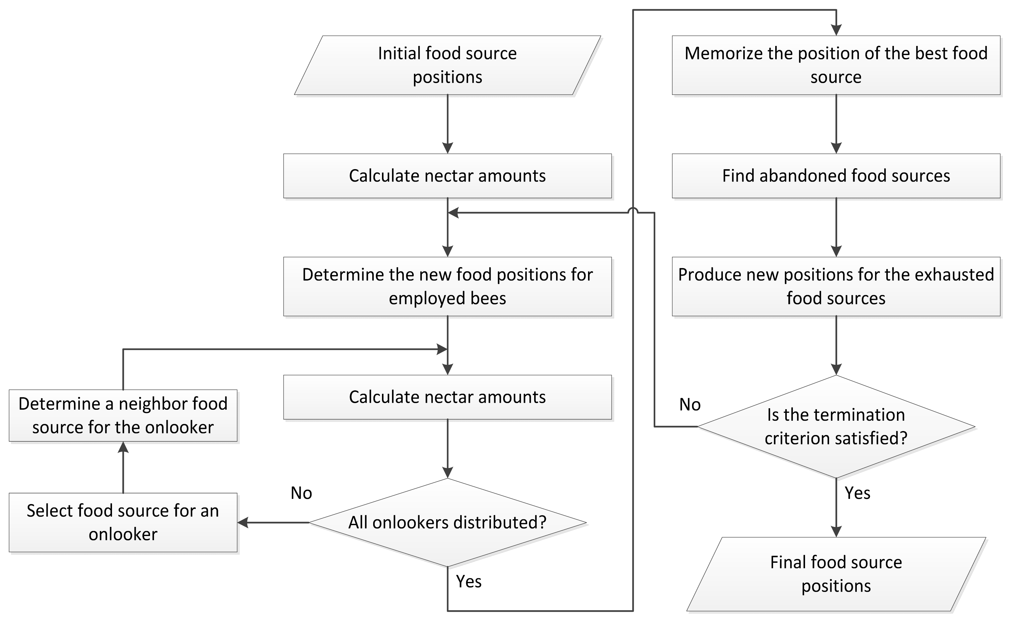
3.1. Artificial Bee Colony

Artificial bee colony is a rather newly developed optimization tool based on the intelligent foraging behavior of honey bee swarm [115–119], and composes several distinct features, e.g., scalability, fault tolerance, adaptation, speed, modularity, autonomy, and parallelism [120], which makes it a potential tool for optimization problems. The main idea of ABC algorithms follows that individual bees are part of a society and have an opinion which is part of a search space shared by every bee. Generally, three groups of bees are considered in the colony. They are employed bees, onlookers and scouts.

In ABC framework, it is assumed to have only one artificial employed bee for each food source. The position of a food source corresponds to a possible solution in the problem’s solution space and the nectar amount of a food source denotes the quality of the associated solution. Each cycle in ABC consists of three different steps: sending the employed bee onto their food sources and evaluating their nectar amounts; after sharing the nectar information of food sources, the selection of food sources regions by the onlookers and evaluating the nectar amount of the food sources; determining the scout bees and then sending them randomly onto possible new food sources. In general, the procedure for the ABC algorithm for continuous problems can be described as follows:

• The initialization phase: The initial solutions are n-dimensional real vectors generated randomly.
• The employed bee phase: Each employed bee is associated with a solution and they apply a random modification (local search) on the solution (assigned food source) to find a new solution (new food source). Once the new food source is obtained, it will be evaluated and compared to the previous. If the fitness of the new solution is better than the previous, the bee will forget the old food source and memorize the new one. Otherwise, she will keep applying modifications until the abandonment criterion is reached.
• The onlooker bee phase: When all employed bees have completed their local search, they share the nectar information of their food source with the onlookers, each of whom will then select a food source in a probabilistic manner. The probability by which an onlooker bee will choose a food source is calculated by:
  $$p_i=\frac{f_i}{{\sum }_{i=1}^{SN}{f}_i}$$

  (6)
  where p_i is the probability by which an onlooker chooses a food source i, SN is the total number of food sources, and f_i is the fitness value of the food source i. The onlooker bees tend to choose the food sources with better fitness value (higher amount of nectar).
• The scout bee phase: If the quality of a solution can’t be improved after a predetermined number of trials (abandonment limit), the food source is abandoned, and the corresponding employed bee becomes a scout. This scout will then produce a randomly generated food source.

All these steps are repeated through a maximum number of cycles (MNC) determined by the user, or until another termination criterion is satisfied. Figure 2 presents a flow chart for implementing the ABC algorithm:

ABC algorithm was developed to solve continuous functions and therefore, certain modifications must be made in order to apply it to combinatorial problem such as scheduling. In broad strokes, the most significant adaptations made to ABC in order to solve the MRCPSP are as follow:

First, everything within the coding is represented in a matrix form. All the activity lists, schedules and all the information related to the benchmark instance is stored as matrices and/or groups of matrices. The second and most important is the modification of the local search, which consists of two operators: swap and insert or both. Refer to Figure 3a,b, where the top row (1,2,4,…, I) represents the identification of activity i, and the bottom row (1,2,3,…,1) represents the mode in which each activity will be executed. Now, supposed we randomly select activity 5 and activity 9 of solution x (Figure 3a) to swap their modes. If this is the case, then activity 5 will be executed in mode 3 instead of mode 2, and activity 9 will now be executed in mode 2, but they will remain in the same order in the schedule, and all other activities will remain with their modes unchanged. If operator insert (Figure 3b) is chosen instead, with the same activities involved (insert mode of activity 9 in 5), then activity 5 will now be executed in mode 3, but this will also change the mode in which the activities between the two activities involved are executed. So, in this example, activity 7 will now be executed in mode 2, activity 11 using mode 2, and activity 9 in mode 1. If mixed operator, swap & insert, is chosen then both of this operators will be executed one after the other.

These operators, however, are not restricted to the mode execution; activities can also be swapped and/or inserted. The difference is that if activities are selected for swap/insert, an internal procedure will schedule them until all their predecessors have been scheduled. So, for example take again activities 5 and 9 selected for a swap but activity 5 is the only predecessor for activity 9. If this is the case, the activity list would follow the order: 1, 2, 4, 7, 11, 5, 9,…, I. Using the operators on both modes and activities helps to extend the solution search space and therefore increases the possibility of finding better solutions.

3.2. Three-Stage Procedure

Before beginning the three-stage procedure, the instance’s information is extracted and its feasibility is evaluated. If feasible then the three-stage procedure will run until the termination criterion is met, otherwise it will continue to randomly select instances until a feasible one is selected.

3.2.1. Stage I—Initial Minimized Makespan Schedule

Part of the complexity in solving the MRCPSP relies in selecting one out of the amount of modes available. In practice, however, we can’t just experiment with all the modes available. We need to select one of the modes available for every activity, preferably based on some kind of rule or parameters which could hopefully optimize either duration, resource consumption or both. In stage I, we generate a population number of initial solutions (schedules) and at least five of these initial solutions are based on modes selected by using Mode Selection Rules. The modes selected for the remaining initial schedules (if more than five) are determined randomly.

3.2.1.1. Mode Selection Rules

At least five of the initial schedules are made with modes selected by using the Mode Selection Rules presented in

Table 1. Mode Selection Rules.

Priority Rule	Description
SFM—Shortest Feasible Mode	Find the feasible mode combination for which the makespan is minimal
LRP—Least Resource Proportion	Choose the mode which leads to the smallest value of the criterion, $\text{max}(\frac{r_{imk}^{\rho }}{K^{\rho }})\forall m$ where $r_{imk}^{\rho }$ stands for the requirement of renewable resource type k per period by activity i executed in mode m. Kρ= total number of renewable resource types in the project.
LPSRD—Least Product Sum of Resource and Duration	For each activity, choose the execution mode which has the minimum product sum of non-renewable resource usage and its corresponding mode duration, $\text{min}{\sum }_{k=1}^{K^v}(r_{imk}^v*d_{im})\forall m$.
LTRU—Least Total Resource Usage	Choose the execution mode which requires the least total non-renewable usage, $\text{min}{\sum }_{k=1}^{K^v}{r}_{imk}^v\forall m$ where $r_{imk}^v$ represents the requirement of non-renewable resource type k per period by activity i executed in mode m. Kv represents the total number of non-renewable resource types in the project.
LRS—Least Sum of Non-renewable Resource	Choose the execution mode which requires the least sum of the ratio of the non-renewable consumption to its corresponding resource limitation, $\text{min}{\sum }_{k=1}^{K^v}\frac{r_{imk}^v}{R_k^v}\forall m$. Here, $R_k^v$ stands for the amount of non-renewable resource type k available per period.

. Shortest Feasible Mode (SFM) and Least Resources proportion were taken from Boctor [121]; the remaining three rules were taken from Chen and Chyu [122]. The mode selection rule to be used is chosen randomly and based on this selection the information of the mode is used to determine the activity list, resource consumption and ultimately, the makespan of the schedule. If population is greater than five then the remaining schedules are made with mode combinations (population–5) determined randomly. The mode combinations found using the MSR could be feasible or infeasible; nonetheless, they are kept in the rest of the procedure because they could become feasible with the local search. On the other hand, all the mode combinations determined randomly always begin as feasible solutions.

Once the execution modes are selected, either by using the MSR or randomly, the next step is to determine the activity lists that will be used in the generation of the initial schedules. The order in which activities are to be scheduled is determined by rules, more specifically Activity Priority Rules.

3.2.1.2. Activity Priority Rules

To establish the order in which every activity will be executed, a priority value derived from the activity priority rules is calculated. The activity to be scheduled next is chosen based on the rule selected and whether the priority value is the largest or smallest. The priority rule used for every solution is selected randomly and they can be found in

Table 2. Activity Priority Rules.

Priority Rule	References	Description
max ACTIM	[123–125]	= CPM – LSTi where CPM stands for the duration of the Critical Path while LST represents the Latest Start Time of activity i.
max GCUMRD	[126]	The sum of the renewable resource demand of the activity considered and the renewable resource demands of all its immediate successors.
max MTS	[127]	| S̄i | the total number of successors for activity i.
max MIS	[127]	| Si | the number of immediate successors for activity i.
max ROT	[128]	$\frac{{\sum }_{k=1}^{K^{\rho }}\frac{r_{ik}^{\rho }}{R_k^{\rho }}}{d_i}$ sum of the ratio of the renewable resource requirement over the resource availability divided by the activity duration for activity i
max WRUP	[129]	$0.7*\mid S_i\mid +0.3*\frac{{\sum }_{k=1}^{K^{\rho }}\frac{r_{ik}^{\rho }}{R_k^{\rho }}}{d_i}$, a weighted sum of the number of immediate successors and an average resource use over all renewable resource types.
min EFT	[130]	EFTi Earliest finish time of activity i.
min LFT	[130]	LFTi Latest finish time of activity i.
min SLK	[130]	LFTi – EFTi
min LNRJ	[126]	| $\overline{N{S}_{\iota }}$| the total number of activities that are not precedence related with activity i
min RSM	[131]	dij = max[0, (EFTi – LSTj)]

:

3.2.1.3. Initial Schedule Generation and Optimization

The final step required within the Initialization Phase of the ABC algorithm is to generate the initial schedules. In this three-stage procedure the schedules are generated using a Serial Generation Scheme (SGS). This means that only one activity is considered at each time and the scheduling order will follow the order provided by the activity list which already considers the information about the activity’s predecessors. Each activity is assigned at the earliest feasible start time.

When all the initial schedules are generated within the initialization phase of ABC, the two improvement phases take place, using the local search operators introduced in Section 3.1. In the Employed Bees Phase, all the solutions are selected for improvement. If a solution is not improved with the local search a counter for solution non-improvement will increase. If a solution is improved its counter will be restarted regardless of the number of non-improvements it had previously. If a solution reaches the abandonment limit for not being improved this solution will be marked for replacement when the Scouts Bees Phase is reached where a new solution will be generated.

The Onlooker Bees Phase makes improvements to solutions based on the probability function described in (6). With higher solution fitness, the probability for it being selected for improvement is increased. Similar to the Employed Bees Phase, if the solution selected is not improved with the local search operators a counter for solution non-improvement will increase but it’s restarted if the solution is improved. If a solution reaches the abandonment limit the solution is marked for replacement by a new solution.

Scouts Bees Phase is the final stage in the ABC algorithm employed. In this stage, all the solutions that reached the abandonment limit are replaced by new solutions. This new solutions can be generated either by using the MSR detailed previously or randomly, the way in which they are determined is selected randomly.

These three improvement phases are performed a maximum number of cycles times and when this criterion is reached, the schedule with the shortest makespan is reported as the lower bound for the three-stage procedure.

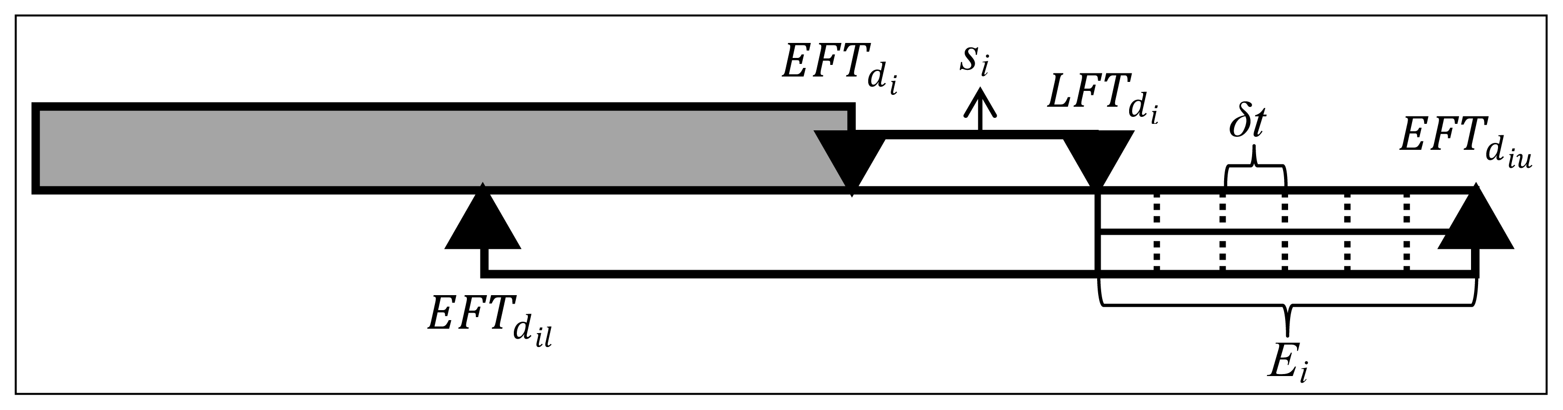
3.3. Stage II—Determining the Schedule’s Entropy

The output for Stage I is a schedule with a minimized makespan which will serve as lower bound for the three-stage procedure. Stage II calculates the activities and schedule’s entropy and with this, a new and possibly—though not necessarily—higher makespan that will serve as an upper bound. The entropy value for each of the activities is calculated using formula (2) as shown in the following example.

Suppose at the end of Stage I we obtain the schedule shown in

Table 3. Example for the Calculation of Activities and a Schedule’s Entropy. (a) Optimized Schedule from Stage I; (b) Range of Estimated Durations; (c) s_i, E_u, S_ID calculation; (d) Resulting Schedule for Stage II.

(a)
Stage I ABC Schedule (Optimized Makespan)
Activity	Start	Duration	Finish
1	0	0	0
3	0	2	2
5	2	7	9
2	0	2	2
4	2	2	4
7	4	4	8
10	9	3	12
8	9	6	15
6	8	2	10
11	15	3	18
9	15	2	17
12	18	0	18

Table 3. Example for the Calculation of Activities and a Schedule’s Entropy. (a) Optimized Schedule from Stage I; (b) Range of Estimated Durations; (c) s_i, E_u, S_ID calculation; (d) Resulting Schedule for Stage II.

(b)
Durations Estimation
Activity	dil	di	diu
1	0	0	0
3	2	2	8
5	7	9	10
2	2	3	5
4	2	6	7
7	4	8	9
10	3	9	9
8	6	7	7
6	2	4	10
11	3	7	8
9	2	4	10
12	0	0	0

Table 3. Example for the Calculation of Activities and a Schedule’s Entropy. (a) Optimized Schedule from Stage I; (b) Range of Estimated Durations; (c) s_i, E_u, S_ID calculation; (d) Resulting Schedule for Stage II.

(c)
Slack, Unfavorable Events and Entropy Calculation
Activity	EST	EFT	LST	LFT	Slack	EFT diu	Eu	SID
1	0	0	0	0	0	0	0	0
3	0	2	17	19	17	8	0	0
5	0	9	0	9	0	10	1	1
2	0	3	3	6	3	5	0	0
4	9	15	9	15	0	16	1	1
7	9	17	14	22	5	18	0	0
10	3	12	6	15	3	12	0	0
8	15	22	15	22	0	22	0	0
6	22	26	22	26	0	32	6	2
11	15	22	19	26	4	23	0	0
9	22	26	22	26	0	32	6	2
12	26	26	26	26	0	26	0	0

Table 3. Example for the Calculation of Activities and a Schedule’s Entropy. (a) Optimized Schedule from Stage I; (b) Range of Estimated Durations; (c) s_i, E_u, S_ID calculation; (d) Resulting Schedule for Stage II.

(d)
Stage II Entropy Containing Schedule (Upper-bound Makespan)
Activity	Start	Duration	Finish
1	0	0	0
3	0	2	2
5	2	8	10
2	0	2	2
4	2	3	6
7	6	4	10
10	10	3	14
8	10	6	16
6	10	4	13
11	16	3	19
9	16	4	19
12	19	0	19

. Table 3b details the scheduler’s estimations for the activity’s shortest possible duration d_il, the most probable duration d_i and the longest possible duration, d_iu. Furthermore, suppose that we are executing our project in a risky environment and therefore we establish daily checkpoints δt = 1. In order to complete the parameters to estimate the entropy we now have to estimate the slack for every activity, following the activity list from the optimized schedule and this is done with the standard forward and backward recursion procedure where EST (LST) is the Earliest (Latest) Start Time and EFT (LFT) is the Earliest (Latest) Finish Time, and EFT _diu is the Earliest Finish Time with the worst possible duration; the results are shown in Table 3c. After the entropy for each activity is calculated, this value is added to the activity’s current duration and with this a new Entropy Containing Schedule is developed as shown in Table 3d.

Let’s take activity 5 as an example, refer to Table 3a. In Stage I, the mode selected for activity 5 determined that its duration will be of 7 time units. In Table 3b we notice that the scheduler determined that the shortest possible duration (d_il) for activity 5 was of 7 time units, the most probable (d_i) was 9 and the longest possible duration (d_iu) was of 10 time units. We run the forward and backward procedure using the most probable duration and we find that activity 5 is part of the critical path for this schedule and therefore has slack s_i = 0. As mentioned previously, this project is being executed in a risky environment and therefore the project manager determines that daily checkpoints are necessary, δt = 1. The EFT _diu is determined by adding the difference between the worst (d_iu) and most probable (d_i) durations to the Earliest Finish Time with the most probable duration (EFT _di), EFT _diu = EFT _di + (d_iu–d_i) and for this case EFT _diu = 10. With Equation (4), we first determine that the set of unfavorable events (E_u) is 1 and using the ceiling function on Equation (2) to avoid fractions of time periods, we find that the entropy for activity 5, S₅ = 1. To form the entropy containing schedule, we add the activity’s entropy values to its current duration and we determine using the same activity list as determined in Stage I we evaluate the new schedule. In our example, the new duration for activity 5 is of 8 time units and after evaluating all the activities, the new makespan for this schedule is 19 time units.

This entropy containing schedule will serve as an upper bound for the makespan in the third and final stage. Notice that even if an activity increases its duration this will not necessarily affect the total makespan of the schedule. For example, notice activity 9, in Stage I the duration was of 2 time units and its entropy increases its duration another 2 time units. Nonetheless, the schedule is only affected in 1 time unit because of the precedence relationships and the activity list determined previously.

3.4. Stage III—Final Robusted Schedule

To produce the robusted schedules, we solve the same model introduced by Talbot [8] and presented in Section 3.1. These robusted schedules, however, instead of minimizing the makespan seek to maximize the robustness while keeping the makespan in a range defined by the boundaries determined in Stage I and Stage II. Recall that Stage I produces a lower bound schedule with minimized makespan (which is not necessarily the lowest makespan the robusted schedule can achieve) while Stage II produces an upper bound makespan by generating an entropy containing schedule. In Stage III, we apply the ABC algorithm again as used in Stage I, but there are 2 major differences:

• In the Initialization phase we keep generating schedules, until the initial population is complete. Contrary to the Initialization phase in Stage I in which the initial makespan of the schedule is irrelevant, in Stage III, only the schedules with initial makespan within the range defined previously are considered as part of the initial population, the rest are discarded.
• The objective function in Stage III maximizes the robustness of the population using Equation (5).

At the end of Stage III, the schedule reported will be one with maximized robustness and with a makespan usually ranging from the lower bound generated in Stage I and at most as high as the entropy containing schedule generated in Stage II. There are cases however, in which the makespan for the robusted schedule is even lower than the lower bound found in Stage I. If this happens, we evaluate if the robustness measure for the Stage III schedule is higher. If so, then this is reported as the result from Stage III. If the makespan is lower but the robustness measure is lower than the Stage I schedule then this schedule is discarded because what we are trying to offer are robust schedules rather than lower makespan. Let’s continue with our previous example to determine the robustness measure. Refer to

Table 7. Results for the evaluation of 40 problem instances for the j10 benchmark set.

No.	Instance	BKO	ABC			ENTROPY			ROBUST
			MS	Dev	RM	MS	Dev	RM	MS	Dev	RM
1	j1020_3	21	21.00	-	44.50	21.00	-	49.25	21.00	-	49.25
2	j108_3	17	18.00	5.88	39.75	26.00	52.94	67.50	18.00	5.88	39.75
3	j1063_5	12	12.00	-	20.00	15.00	25.00	105.75	12.00	-	45.25
4	j1046_10	20	20.00	-	64.25	24.00	20.00	101.50	20.00	-	66.25
5	j1037_3	29	27.00	(6.90)	73.00	29.00	-	80.50	26.00	(10.34)	75.25
6	j1031_6	20	20.00	-	40.00	21.00	5.00	55.50	20.00	-	61.25
7	j104_9	21	17.00	(19.05)	32.50	23.00	9.52	37.00	17.00	(19.05)	32.50
8	j1055_1	18	18.00	-	80.00	21.00	16.67	87.00	19.00	5.56	82.00
9	j103_3	19	18.00	(5.26)	39.50	19.00	-	47.25	18.00	(5.26)	39.50
10	j1016_10	26	26.00	-	39.00	27.00	3.85	42.50	26.00	-	69.25
11	j1020_4	17	17.00	-	28.00	17.00	-	30.00	17.00	-	53.75
12	j1036_1	32	32.00	-	82.50	36.00	12.50	93.75	32.00	-	82.50
13	j1018_2	15	15.00	-	21.75	17.00	13.33	31.50	15.00	-	23.25
14	j1063_3	17	17.00	-	73.25	20.00	17.65	79.00	18.00	5.88	105.25
15	j1060_1	13	13.00	-	21.00	15.00	15.38	62.75	13.00	-	34.25
16	j1029_10	28	26.00	(7.14)	31.00	28.00	-	33.00	27.00	(3.57)	59.25
17	j1026_2	12	12.00	-	23.50	14.00	16.67	34.00	11.00	(8.33)	25.50
18	j1018_6	15	15.00	-	28.00	16.00	6.67	30.50	15.00	-	35.00
19	j1043_6	16	16.00	-	32.50	21.00	31.25	32.50	16.00	-	85.75
20	j1062_4	15	15.00	-	69.50	15.00	-	73.50	15.00	-	85.25
21	j107_5	24	24.00	-	39.00	26.00	8.33	44.25	25.00	4.17	41.00
22	j1029_10	28	28.00	-	40.50	30.00	7.14	59.75	27.00	(3.57)	48.50
23	j1028_10	18	18.00	-	60.25	22.00	22.22	72.00	22.00	22.22	90.25
24	j1014_2	19	19.00	-	41.50	21.00	10.53	79.75	19.00	-	77.50
25	j1010_6	18	17.00	(5.56)	28.75	18.00	-	32.25	14.00	(22.22)	42.00
26	j1036_5	23	21.00	(8.70)	73.50	24.00	4.35	80.50	15.00	(34.78)	73.50
27	j1044_9	17	17.00	-	62.50	21.00	23.53	66.00	17.00	-	62.50
28	j1023_8	18	18.00	-	40.00	20.00	11.11	46.75	18.00	-	49.50
29	j1018_3	17	16.00	(5.88)	38.00	18.00	5.88	40.00	16.00	(5.88)	38.00
30	j1034_4	23	23.00	-	41.00	25.00	8.70	42.75	23.00	-	74.75
31	j1026_4	16	16.00	-	28.00	18.00	12.50	38.75	18.00	12.50	38.75
32	j103_7	14	14.00	-	10.00	20.00	42.86	18.00	15.00	7.14	27.50
33	j1063_2	17	17.00	-	71.00	22.00	29.41	163.25	17.00	-	135.50
34	j1042_5	20	21.00	5.00	101.00	25.00	25.00	124.50	22.00	10.00	120.25
35	j1014_1	16	17.00	6.25	43.75	19.00	18.75	54.25	17.00	6.25	90.25
36	j1010_9	10	10.00	-	27.00	11.00	10.00	49.75	11.00	10.00	49.75
37	j1045_10	25	26.00	4.00	120.50	27.00	8.00	127.50	27.00	8.00	141.75
38	j1050_4	20	19.00	(5.00)	116.00	23.00	15.00	128.50	19.00	(5.00)	140.75
39	j1051_7	21	21.00	-	81.25	23.00	9.52	86.25	21.00	-	81.25
40	j1060_8	13	13.00	-	40.00	14.00	7.69	101.75	13.00	-	40.00

.

Table 4. Example for the Calculation of Activities and a Schedule’s Entropy. (a) Optimized Makespan—Stage I; (b) Entropy Containing Schedule—Stage II; (c) Schedules generated during Initialization Phase in Stage III; (d) Final Robust Schedule generated in Stage III.

(a)
Stage I ABC Schedule (Lower Bound)
Activity	Start	Duration	Finish	RM
1	0	0	0	67.25
3	0	2	2	67.25
5	2	7	9	67.25
2	0	2	2	67.25
4	2	2	4	67.25
7	4	4	8	67.25
10	9	3	12	67.25
8	9	6	15	67.25
6	8	2	10	67.25
11	15	3	18	67.25
9	15	2	17	67.25
12	18	0	18	67.25

Table 4. Example for the Calculation of Activities and a Schedule’s Entropy. (a) Optimized Makespan—Stage I; (b) Entropy Containing Schedule—Stage II; (c) Schedules generated during Initialization Phase in Stage III; (d) Final Robust Schedule generated in Stage III.

(b)
Stage II Entropy Containing Schedule (Upper Bound)
Activity	Start	Duration	Finish	RM
1	0	0	0	93.5
3	0	2	2	93.5
5	2	8	10	93.5
2	0	2	2	93.5
4	2	3	6	93.5
7	6	4	10	93.5
10	10	3	14	93.5
8	10	6	16	93.5
6	10	4	13	93.5
11	16	3	19	93.5
9	16	4	19	93.5
12	19	0	19	93.5

Table 4. Example for the Calculation of Activities and a Schedule’s Entropy. (a) Optimized Makespan—Stage I; (b) Entropy Containing Schedule—Stage II; (c) Schedules generated during Initialization Phase in Stage III; (d) Final Robust Schedule generated in Stage III.

(c)
Activity	Start	Duration	Finish	Activity	Start	Duration	Finish
1	0	0	0	1	0	0	0
4	0	2	2	3	0	2	2
3	0	2	2	5	2	7	9
6	2	2	4	2	0	2	2
5	2	7	9	6	2	2	4
7	4	4	8	4	4	2	6
8	9	6	15	7	6	4	10
9	15	2	17	10	9	3	12
11	15	3	18	8	10	6	16
2	8	2	10	11	16	3	19
10	10	3	13	9	16	2	18
12	18	0	18	12	19	0	19
1	0	0	0	1	0	0	0
2	0	2	2	3	0	2	2
3	0	2	2	2	0	2	2
5	2	7	9	6	2	2	4
4	2	2	4	5	2	7	9
6	4	2	6	4	4	2	6
7	6	4	10	10	9	3	12
10	9	3	12	7	6	4	10
8	10	6	16	8	10	6	16
9	16	2	18	9	16	2	18
11	16	3	19	11	16	3	19
12	19	0	19	12	19	0	19

Table 4. Example for the Calculation of Activities and a Schedule’s Entropy. (a) Optimized Makespan—Stage I; (b) Entropy Containing Schedule—Stage II; (c) Schedules generated during Initialization Phase in Stage III; (d) Final Robust Schedule generated in Stage III.

(d)
Stage III Robusted Schedule (FINAL)
Activity	Start	Duration	Finish	RM
1	0	0	0	93.5
4	0	2	2	93.5
3	0	2	2	93.5
6	2	2	4	93.5
5	2	7	9	93.5
7	4	4	8	93.5
8	9	6	15	93.5
9	15	2	17	93.5
11	15	3	18	93.5
2	8	2	10	93.5
10	10	3	13	93.5
12	18	0	18	93.5

show the schedule reported in Stage I with Robustness Measure (RM) = 67.25 and Stage II with Robustness Measure = 93.5 respectively. To calculate this measure we need to define parameter frac (for this example it was set as 0.25) which stands for 25% of the duration of activity i in mode m. The robustness measure will take the minimum between the activity’s total slack and the value of (min (s_i, frac*d_i)) and later multiply it by the number of successors and resource used in mode m. Table 4c demonstrates four different schedules generated in the Initialization Phase for Stage III. Finally, Table 4d presents the schedule with maximized robustness that will be reported at the end of Stage III.

4. Computational Results

4.1. Scope

To evaluate the practicality of our approach we conducted experiments solving the test instances generated by the ProGen and collected in the PSPLIB [132]. In this benchmark, each set of instances contain 2 renewable and 2 non-renewable resources and the number of activities goes from 10, 12, 14, 16, 18, 20 and up to 30, being 30 activities the most complicated to solve. Every activity, except for the dummies (i = 1 and i = I), has 3 modes in which they can be executed. As the number of activities increases, the possible mode combinations increase exponentially, starting from 59,049 when the number of activities is 10 and rising up to 2.05891E+14 when working with 30 activities.

Also, in an effort to solve larger instances, we used the MRCPSP/max benchmark set collected in [133]. The instances in these sets contain 50 or 100 activities respectively; use three renewable, three non-renewable and three doubly constrained resources; and every activity can be executed in at least three and in up to five different modes. However; there are significant differences regarding the constraints when compared to the MRCPSP we are solving for this paper. In order to sort through these differences and be able to use most of the information (number of activities, resources and some of the network structure) we had to pre-process the data and disconnect loops between successors and predecessors which are not considered in the original MRCPSP. Nonetheless, this process affects almost completely the way in which most of the activities are interconnected originally from beginning to end. This in turn affects the gap between solutions obtained with the ABC algorithm and the best known solutions because by changing the network, it’s essentially a different problem. And even though comparing solutions for what are basically different problems is unfair and not as promising as when compared when solving the original MRCPSP, we still compare against the MRCPSP/max best known solutions because these are our only objective point of reference and we also consider this could be the worst case scenario.

The experiments were very straight-forward, following the procedures described in Section 3 and the only additional information used were the parameters used to evaluate the formulas. The purpose of this study is to develop an approach that basically generates a lower and upper bound for a schedule’s makespan and ultimately generate a robust baseline schedule within these boundaries which is capable of absorbing variations caused by its inherent uncertainty. And even though our main objective was not to minimize the makespan, in most of the MRCPSP cases in the PSPLIB the best-known solution was reached as the lower bound. Also, it is worth to mention that in practically every set of these instances at least one better solution was found. On the other hand, the results for the MRCPSP/max were not as promising as when solving the original MRCPSP and for these sets the best-known solution was not achieved for any of the instances solved. Again, we consider this is due to the pre-processing done and the change in the relationships between activities.

4.2. Description of the Procedure

The first step in our procedure was to conduct a short sensitivity analysis where a total of five parameters, each with three different levels, were tested. At each test, only one specific parameter changed its level while the remaining four parameters were kept at their base level. The base levels were chosen empirically; however, their values are the strictest possible settings among the levels. This means that the higher levels were chosen for parameters that increase the search space or number of solutions evaluated (population size and MNC); while the lowest and most quality demanding levels were chosen for those parameters that are linked directly to the solution’s quality (abandonment limit, δt, frac).

Table 5. Parameters and levels for sensitivity analysis.

Parameter	Settings (* base level)
Population size	5	15	30*
Abandonment limit	5*	10	15
MNC	5	10	20*
δt (relevant time interval)	1*	2	3
frac	0.25*	0.50	0.75

shows the levels chosen to conduct the sensitivity analysis.

The sensitivity analysis was performed on every set of benchmark instances. As an example,

Table 6. Sensitivity Analysis Result for one problem instance of j10 benchmark set.

		Deviation when compared to Optimal Makespan (%)			Deviation when compared to ABC Makespan (%)
		ABC Schedule	Entropy Schedule	Robust Schedule	Entropy Schedule	Robust Schedule
Population Size	5	33.33	55.56	50.00	16.67	12.50
	15	6.67	20.00	20.00	12.50	12.50
	30	-	6.67	6.67	6.67	6.67
Abandonment Limit	5	-	6.67	6.67	6.67	6.67
	10	26.67	46.67	46.67	15.79	15.79
	15	31.82	45.45	31.82	10.34	-
MNC	5	7.69	23.08	23.08	14.29	14.29
	10	4.55	4.55	4.55	-	-
	20	-	6.67	6.67	6.67	6.67
δt (relevant time interval)	3	95.00	130.00	100.00	17.95	2.56
	2	18.75	37.50	37.50	15.79	15.79
	1	-	6.67	6.67	6.67	6.67
Frac	0.25	-	6.67	6.67	6.67	6.67
	0.5	26.67	46.67	46.67	15.79	15.79
	0.75	31.82	45.45	31.82	20.00	-
MNC	5	7.69	23.08	23.08	14.29	14.29
	10	4.55	4.55	4.55	-	-
	20	-	6.67	6.67	6.67	6.67
δt (relevant time interval)	3	95.00	130.00	100.00	17.95	2.56
	2	18.75	37.50	37.50	15.79	15.79
	1	-	6.67	6.67	6.67	6.67
Frac	0.25	-	6.67	6.67	6.67	6.67
	0.5	26.67	46.67	46.67	15.79	15.79
	0.75	31.82	45.45	31.82	20.00	-

shows the results of the sensitivity analysis when performed for one of the problem instances on j10. The values marked in grey represent the base level used for the sensitivity analysis. The deviation between makespan was determined by (M_s–M*)/M* where M* represents the optimal or best-known makespan and M_s denotes the makespan of the schedule against which it is being compared. When comparing the ABC against the entropy schedules and robust schedule, M* refers to the makespan achieved for the ABC schedule. The same analysis was performed on the rest of the benchmark sets and the results confirm our empirical choice for the base level settings. The best results (when comparing ABC Schedule vs. Optimal Makespan) are obtained when using higher levels on parameters that increase the search space and using the lowest levels for those parameters that are linked directly to the solution’s quality.

4.3. Results

After determining the levels for the parameters (Population Size: 30, Abandonment Limit: 5, MNC: 20, δt: 1, frac: 0.25), we proceeded to run our experiments on every benchmark set. The algorithm cycles through the total problem instances available for each set, and randomly selects a predetermined number of feasible instances to be solved and compared against their best-known solutions. Even though in the case of MRCPSP/max we are essentially solving a different. Table 7 shows an example of the results obtained when evaluating the j10 benchmark set. The description of this table is as follows: Column BKO indicates the best-known solution for the problem instance; ABC, ENTROPY and ROBUST indicate the kind of schedule being compared against the BKO and under each of them we find the columns: MS which stands for makespan of that particular schedule, Dev which is the deviation of the schedule’s makespan when compared to BKO and RM which represents the robustness measure obtained for the schedule. The numbers highlighted indicate that a solution better than the BKO was achieved either in the ABC schedule or in the robust schedule and therefore, the deviation is shown in parentheses to indicate a negative value. Recall that the ROBUST schedule is independent of the ABC schedule generated and the only hard restriction is that its makespan should be at most as high as the ENTROPY makespan.

Similarly to the sensitivity analysis, this same table was generated for all the remaining benchmark sets and for each of them we evaluated if the deviation is statistically equal to 0 in case of the ABC schedule and if it’s statistically equal to 10 in the case of the Entropy and Robust Schedules.

When solving for the MRCPSP/max benchmark set we evaluate if the deviation is statistically equal to 25 in case of the ABC schedule and if it’s statistically equal to 35 in the case of the Entropy and Robust Schedules. When solving for the MRCPSP, the selection for the hypotheses values was based on values which are lower than the typical buffers used in practice. From previous field experience, a typical project buffer consists of adding (rather subjectively) a value of 10 and up to 20% of the estimated initial budget depending on the uncertainty under which the project is being executed. For this research, we wanted to prove that to objectively define a robust schedule is possible, and even a duration range is better than the values used in practice.

Regarding the values for the MRCPSP/max, it would not be a fair comparison to use the same hypotheses values because as aforementioned, the problem has different constraints and the preprocessing of the data alters the expected performance of the algorithm.

Table 8. Results for the evaluation of 40 problem instances for the MRCPSP and MRCPSP/max benchmark set.

Summarized Results for Benchmark Evaluations
		j10	j12	j14	j16	j18	j20	j30	mm50	mm100
ABC	Avg. Dev.	(1.06)	0.41	3.43	3.36	2.12	5.78	9.61	24.72	32.94
	Std. Dev.	4.31	4.89	7.99	8.55	5.46	8.89	12.39	7.50	11.54
	Avg. RM.	49.68	71.93	107.51	121.25	134.01	154.83	251.03	840.56	963.99
	Improved BKO’s	8.00	11.00	7.00	7.00	4.00	4.00	-	-	-
	p-value	0.13	0.60	0.01	0.02	0.02	0.00	0.73	0.07	0.04
	95% CI. Lower Bound	(2.44)	(1.17)	0.84	0.59	0.35	2.91	(3.53)	10.13	18.31
	95% CI. Upper Bound	0.32	2.00	6.02	6.13	3.89	8.66	2.50	29.20	60.59
ENTROPY	Avg. Dev.	13.17	15.05	17.85	16.52	13.49	18.88	21.11	39.99	69.10
	Inc. Avg. Dev. (x)	13.44	35.43	4.20	3.92	5.37	2.26	1.20	0.62	1.10
	Std. Dev.	11.60	13.76	12.49	12.62	10.35	11.74	13.57	12.30	24.28
	Avg. RM.	65.77	95.91	124.84	153.76	167.16	195.62	293.59	1,030.88	1,573.40
	Inc. Avg. RM. (%)	32.40	33.34	16.12	26.81	24.73	26.35	16.96	22.64	40.32
	p-value	0.10	0.03	0.00	0.00	0.04	<.0001	<.0001	0.35	<.0001
	95% CI. Lower Bound	9.42	10.60	13.80	12.43	10.14	15.08	(1.31)	30.79	53.20
	95% CI. Upper Bound	16.93	19.51	21.89	20.61	16.84	22.68	3.78	48.78	87.06
ROBUST	Avg. Dev.	(0.51)	1.24	12.94	11.61	8.33	11.08	10.96	30.37	53.66
	Inc. Avg. Dev.	(0.52)	1.99	2.77	2.46	2.93	0.92	0.14	0.23	0.63
	Std. Dev.	9.31	7.85	9.36	11.39	7.64	8.79	12.81	9.59	18.78
	Avg. RM.	65.33	91.03	131.39	152.62	168.15	192.63	276.25	1,012.07	1,363.76
	Inc. Avg. RM. (%)	31.52	26.56	22.21	25.87	25.47	24.42	10.05	20.40	31.17
	Improved BKO’s	7.00	11.00	1.00	1.00	1.00	1.00	-	-	-
	ROB = ABC or ROB = ENT	11.00	8.00	10.00	20.00	17.00	14.00	19.00	16.00	18.00
	p-value	<.0001	<.0001	0.06	0.38	0.18	0.45	0.06	0.05	0.01
	95% CI. Lower Bound	(3.53)	(1.31)	9.90	7.92	5.85	8.23	9.90	29.46	41.32
	95% CI. Upper Bound	2.50	3.78	15.97	15.30	10.80	13.93	15.97	46.59	67.61

summarizes the results achieved for all the benchmark sets. Here rows ABC, ENTROPY and ROBUST summarize the results achieved during Stage I, Stage II and Stage III, respectively, while the columns define the benchmark set in which the results were obtained. The row Avg. Dev. represents the Average Deviation obtained from the instances solved, Std. Dev. is the Standard Deviation of the average deviations, and Avg. RM stands for the Average Robustness of the 40 schedules. The number of solutions that were improved when compared to the BKO is registered in the row Improved BKO’s while row p-value is the criterion to evaluate our hypotheses. Furthermore, the rows 95% CI shows the lower and upper bound for the 95% confidence interval of the Avg. Dev estimation. In the ENTROPY and ROBUST sections, we have 2 extra rows that measure the increase in the average deviation and in the robustness with respect to the ABC schedule. ROBUST also includes a row that counts the times in which the robusted schedule is equal to either the ABC schedule or the Entropy schedule. Just as in Table 7, the negative values here are shown in parenthesis.

Given the differences in the benchmark information and the significant differences in results, we will discuss the results for the MRCPSP and the MRCPSP/max separately. First, regarding the MRCPSP and based on the summary for columns j10–j30 presented in Table 8 we can make the following claims: we can conclude with a 95% of confidence that for the instances solved the Avg. Dev. when trying to minimize the makespan (Stage I—ABC schedule) will not exceed 8.66% in the worst case, and its upper bound will be around 4%, on average. With a 95% confidence the upper limit for the Avg. Dev. on the Entropy schedule (Stage II) will be 22.68% in the worst case while 17% on average when compared to the BKO. Keep in mind, however, that the schedule for Stage II is based on Stage I, and so the increase in Avg. Dev. when compared to the ABC schedule is on average only 9.4% while the average increase on robustness is 25% and up to 33%.

For Stage III we can observe with a 95% confidence that the upper limit will not exceed 16% regardless of the benchmark tested. The average deviation when compared to the BKO is 7.95%, and only 1.52% when compared to the ABC schedule generated in Stage I. The average increase in robustness is 23% and it goes up to 31%. Also, with the 40 instances solved for each set, the schedule generated in Stage III fell in one of the limits (Stage I or Stage II) in at most 50% of the cases, and just as in Stage I, an improvement on the BKO was made in practically every benchmark set.

These results, lead us to conclude that although ABC was initially developed to solve continuous problems, making the right adjustments proves that it is a powerful meta-heuristic algorithm to work on discrete problems as well.

Now, regarding the results for MRCPSP/max mm50 and mm100 recall our hypotheses for Stage I (ABC Schedule):

From the results in Table 8, we cannot reject our null hypothesis for the mm50 set which states that the average deviation with respect to the best-known solutions is 25. And we can state with a 95% confidence that the Avg. Dev. will range from 10.13 up to 29.20. For the mm100 set however, we reject our null hypothesis and our 95% confidence goes from 18.31 to 60.59. For Stage II and Stage III, we stated the following hypotheses:

Based on Table 8, we reject the null hypothesis in both stages for instances solved of the mm100 but we fail to reject the null hypotheses for the mm50 set. The Entropy Schedule for the mm50 instances solved has an Avg. Dev. of 39.99, which represents a 0.62 increase with respect to the ABC Schedule from Stage I. The increase in RM on the other hand is a significant 22.64% from the initial schedule. The Robust Schedule has an Avg. Dev. of 30.37, and in the worst case it will be 46.59 while 29.46 on the best case with an average increase in RM of 20.40%. Also, 16 of the schedules generated in this stage falls in either one of the boundaries.

5. Conclusions

The main purpose of this study was to introduce an approach to generate baseline schedules that are capable of absorbing variations caused by the uncertain environment in which they have to be executed. The impact of this methodology is significant in the sense that it allows project managers to easily estimate a range in which a schedule can be completed without adding any personal judgment into the evaluation. This range is only dependent on the nature of the environment—whether it is very uncertain or relatively stable—the durations estimated for every activity and the way in which the activities are interconnected. We evaluate this approach by solving the MRCPSP and the MRCPSP/max benchmark sets and the computational results show that for the MRCPSP set it is possible to generate robust baseline schedules with an increase of at most 16% with respect to the best-known solutions but which are statistically less than or equal to 10% for every set. For the MRCPSP/max benchmark sets we speculate that the significant difference in results derives from the way in which the instances were generated. For these sets, the relationships between activities violate constraints established in the original MRCPSP being solved in this paper and therefore trying to solve it with the exact same algorithm does not result in the same promising results as with the MRCPSP. However, the approach in general is still applicable and we will use this benchmark sets for future researches as it does present an even more realistic scenario within project management.

References

1. Turner, J.R. The Handbook of Project Based Management; McGraw-Hill: London, UK, 1993. [Google Scholar]
2. Turner, J.R. The Handbook of Project Based Management, 2nd ed; McGraw-Hill: London, UK, 1999. [Google Scholar]
3. Turner, J.R.; Müller, R. On the nature of the project as a temporary organization. Int. J. Proj. Manag 2003, 21, 1–8. [Google Scholar]
4. Blazewicz, J.; Lenstra, J.K.; Kan, A.H.G. Scheduling subject to resource constraints: Classification and complexity. Discret. Appl. Math 1983, 5, 11–24. [Google Scholar]
5. Kolisch, R. Project Scheduling under Resource Constraints—Efficient Heuristics for Several Problem Cases; Physica-Verlag: Heidelberg, Germany, 1995. [Google Scholar]
6. Elmaghraby, S.E. Activity Networks: Project Planning and Control by Network Models; Wiley: New York, NY, USA, 1977. [Google Scholar]
7. Kolisch, R.; Drexl, A. Local search for a non-preemptive multimode resource constrained project scheduling. IIE Trans 1997, 29, 987–999. [Google Scholar]
8. Talbot, B. Resource-constrained project scheduling with time resource tradeoffs: The nonpreemptive case. Manag. Sci 1982, 28, 1197–1210. [Google Scholar]
9. De Reyck, B.; Demuelemeester, E.L.; Herroelen, W.S. Local search methods for the discrete time/resource trade-off problem in project networks. Nav. Res. Logist. Q 1998, 45, 553–578. [Google Scholar]
10. Pollack-Johnson, B.; Liberatore, M.J. Incorporating quality considerations into project time/cost trade-off analysis and decision making. IEEE Trans. Eng. Manag 2006, 53, 31–37. [Google Scholar]
11. Ranjbar, M.; De Reyck, B.; Kianfar, F. A hybrid scatter search for the discrete time/resource trade-off problem in project scheduling. Eur. J. Oper. Res 2009, 193, 35–48. [Google Scholar]
12. Özdamar, L.; Ulusoy, G.; Bayyigit,, M. A heuristic treatment of tardiness and net present value criteria in resource constrained project scheduling. Int. J. Phys. Distrib. Logist. Manag 1998, 28, 805–824. [Google Scholar]
13. Pesch, E. Lower bounds in different problem classes of project schedules with resource constraints. In Project Scheduling: Recent Models, Algorithms and Applications; Weglarz, J., Ed.; Kluwer Academic Publishers: Springer US, New York, NY, USA, 1999; pp. 53–76. [Google Scholar]
14. Hartmann, S.; Drexl, A. Project scheduling with multiple modes: A comparison of exact algorithms. Networks 1998, 32, 283–297. [Google Scholar]
15. Józefowska, J.; Micka, M.; Rózycki, R.; Waligóra, G. Simulated annealing for multi-mode resource-constrained project scheduling. Ann. Oper. Res 2001, 102, 117–155. [Google Scholar]
16. Alcaraz, J.; Maroto, C.; Ruiz, R. Solving the multimode resource constrained project scheduling problem with genetic algorithms. J. Oper. Res. Soc 2003, 54, 614–626. [Google Scholar]
17. Bouleimen, K.; Lecocq, H. A new efficient simulated annealing algorithm for the resource-constrained project scheduling problem and its multiple mode version. Eur. J. Oper. Res 2003, 149, 268–281. [Google Scholar]
18. Jarboui, B.; Damak, N.; Siarry, P.; Rebai, A. A combinatorial particle swarm optimization for solving multi-mode resource-constrained project scheduling problems. Appl. Math. Comput 2008, 195, 299–308. [Google Scholar]
19. Nudtasomboon, N.; Randhawa, S.U. Resource-constrained project scheduling with renewable and non-renewable resources and time-resource tradeoffs. Comput. Ind. Eng 1997, 32, 227–242. [Google Scholar]
20. Salewski, F.; Schirmer, A.; Drexl, A. Project scheduling under resource and mode identity constraints: Model, complexity, methods, and application. Eur. J. Oper. Res 1997, 102, 88–110. [Google Scholar]
21. Drexl, A.; Nissen, R.; Patterson, J.H.; Salewski, F. Progen/px—An instance generator for resource-constrained project scheduling problems with partially renewable resources and further extensions. Eur. J. Oper. Res 2000, 125, 59–72. [Google Scholar]
22. Erenguc, S.S.; Ahn, T.; Conway, D.G. The resource constrained project scheduling problem with multiple crashable modes: An exact solution method. Nav. Res. Logist 2001, 48, 107–127. [Google Scholar]
23. Bellenguez, O.; Néron, E. Lower bounds for the multi-skill project scheduling problem with hierarchical levels of skills. Lect. Notes Comput. Sci 2005, 3616, 229–243. [Google Scholar]
24. Zhu, G.; Bard, J.F.; Yu, G. A branch-and-cut procedure for the multimode resource-constrained project-scheduling problem. INFORMS J. Comput 2006, 18, 377–390. [Google Scholar]
25. Varma, V.A.; Uzsoy, R.; Pekny, J.; Blau, G. Lagrangian heuristics for scheduling new product development projects in the pharmaceutical industry. J. Heuristics 2007, 13, 403–433. [Google Scholar]
26. De Reyck, B.; Herroelen, W.S. The multi-mode resource-constrained project scheduling problem with generalized precedence relations. Eur. J. Oper. Res 1999, 119, 538–556. [Google Scholar]
27. Heilmann, R. Resource-constrained project scheduling: A heuristic for the multi-mode case. OR Spektrum 2001, 23, 335–357. [Google Scholar]
28. Heilmann, R. A branch-and-bound procedure for the multi-mode resource-constrained project scheduling problem with minimum and maximum time lags. Eur. J. Oper. Res 2003, 144, 348–365. [Google Scholar]
29. Nonobe, K.; Ibaraki, T. Formulation and tabu search algorithm for the resource constrained project scheduling problem. In Essays and Surveys in Metaheuristics; Ribeiro, C.C., Hensen, P., Eds.; Kluwer Academic Publishers: Norwell, MA, US, 2002; pp. 557–588. [Google Scholar]
30. Brucker, P.; Knust, S. Resource-constrained project scheduling and timetabling. In The Practice and Theory of Automated Timetabling III; Burke, E., Erben, W., Eds.; Springer: Berlin/Heidelberg, 2001; Volume 2079, pp. 277–293. [Google Scholar]
31. Calhoun, V.D.; Pekar, J.J.; McGinty, V.B.; Adali, T.; Watson, T.D.; Pearlson, G.D. Different activation dynamics in multiple neural systems during simulated driving. Hum. Brain Mapp 2002, 16, 158–167. [Google Scholar]
32. Sabzehparvar, M.; Seyed-Hosseini, S.M. A mathematical model for the multi-mode resource-constrained project scheduling problem with mode dependent time lags. J. Supercomput 2008, 44, 257–273. [Google Scholar]
33. Barrios, A.; Ballestin, F.; Valls, V. A double genetic algorithm for the MRCPSP/max. Comput. Oper. Res 2011, 38, 33–43. [Google Scholar]
34. Tareghian, H.R.; Taheri, S.H. A solution procedure for the discrete time, cost and quality tradeoff problem using electromagnetic scatter search. Appl. Math. Comput 2007, 190, 1136–1145. [Google Scholar]
35. Li, H.; Womer, K. Modeling the supply chain configuration problem with resource constraints. Int. J. Proj. Manag 2008, 26, 646–654. [Google Scholar]
36. Tiwari, V.; Patterson, J.H.; Mabert, V.A. Scheduling projects with heterogeneous resources to meet time and quality objectives. Eur. J. Oper. Res 2009, 193, 780–790. [Google Scholar]
37. Bonfill, A.; Espuña, L.; Puigjaner, L. Proactive approach to address the uncertainty in short-term scheduling. Comput. Chem. Eng 2008, 32, 1689–1706. [Google Scholar]
38. Kolisch, R.; Padman, R. An integrated survey of deterministic project scheduling. Omega 2001, 29, 249–272. [Google Scholar]
39. Franck, B.; Schwindt, C. Different Resource-constrained Project Scheduling Models with Minimal and Maximal Time-lags; Technical Report WIOR-450; Universität Karlsruhe: Karlsruhe, Germany, 1995. [Google Scholar]
40. Vanhoucke, M.; Demeulemeester, E.L.; Herroelen, W.S. An exact procedure for the resource-constrained weighted earliness-tardiness project scheduling problem. Ann. Oper. Res 2001, 102, 179–196. [Google Scholar]
41. Neumann, K.; Schwindt, C.; Zimmermann, J. Recent results on resource-constrained project scheduling with time windows: Models, solution methods, and applications. Cent. Eur. J. Oper. Res 2002, 10, 113–148. [Google Scholar]
42. Lorenzoni, L.L.; Ahonen, H.; de Alvarenga, A.G. A multi-mode resource-constrained scheduling problem in the context of port operations. Comput. Ind. Eng 2006, 50, 55–65. [Google Scholar]
43. Kolisch, R. Integrated scheduling, assembly area- and part-assignment for large-scale, make-to-order assemblies. Int. J. Prod. Econ 2000, 64, 127–141. [Google Scholar]
44. Viana, A.; de Sousa, J.P. Using meta-heuristics in multi-objective resource constrained project scheduling. Eur. J. Oper. Res 2000, 120, 359–374. [Google Scholar]
45. Ballestin, F.; Valls, V.; Quintanilla, S. Due Dates and RCPSP. In International Series in Operations Research & Management Science; Józefowska, J., Weglarz, J., Eds.; Springer: New York City, US, 2006; Volume 92, pp. 79–104. [Google Scholar]
46. Rom, W.O.; Icmeli-Tuckel, O.; Muscatello, J.R. MRP in a job shop environment using a resource constrained project scheduling model. Omega 2002, 30, 275–286. [Google Scholar]
47. Nazareth, T.; Verma, S.; Bhattacharya, S.; Bagchi, A. The multiple resource constrained project scheduling problem: A breadth-first approach. Eur. J. Oper. Res 1999, 112, 347–366. [Google Scholar]
48. Vanhoucke, M. Scheduling an R&D project with quality-dependent time slots. Lect. Notes Comput. Sci 2006, 3982, 621–630. [Google Scholar]
49. Maniezzo, V.; Mingozzi, A. The project scheduling problem with irregular starting time costs. Oper. Res. Lett 1999, 25, 175–182. [Google Scholar]
50. Möhring, R.H.; Schulz, A.S.; Stork, F.; Uetz, M. On project scheduling with irregular starting time costs. Oper. Res. Lett 2001, 28, 149–154. [Google Scholar]
51. Möhring, R.H.; Schulz, A.S.; Stork, F.; Uetz, M. Solving project scheduling problems by minimum cut computations. Manag. Sci 2003, 49, 330–350. [Google Scholar]
52. Achuthan, N.; Hardjawidjaja, A. Project scheduling under time dependent costs—A branch and bound algorithm. Ann. Oper. Res 2001, 108, 55–74. [Google Scholar]
53. Dodin, B.; Elimam, A.A. Integrated project scheduling and material planning with variable activity duration and rewards. IIE Trans 2001, 33, 1005–1018. [Google Scholar]
54. Nonobe, K.; Ibaraki, T. Chapter 9. A metaheuristic approach to the resource constrained project scheduling with variable activity durations and convex cost functions. In International Series in Operations Research & Management Science; Józefowska, J., Weglarz, J., Eds.; Springer: New York, NY, USA, 2006; Volume 92, pp. 225–248. [Google Scholar]
55. Kimms, A. Maximizing the net present value of a project under resource constraints using a Lagrangian relaxation based heuristic with tight upper bounds. Ann. Oper. Res 2001, 102, 221–236. [Google Scholar]
56. Vanhoucke, M.; Demeulemeester, E.L.; Herroelen, W.S. On maximizing the net present value of a project under renewable resource constraints. Manag. Sci 2001, 47, 1113–1121. [Google Scholar]
57. Mika, M.; Waligóra, G.; Weglvarz, J. Simulated annealing and tabu search for multi-mode resource-constrained project scheduling with positive discounted cash flows and different payment models. Eur. J. Oper. Res 2005, 164, 639–668. [Google Scholar]
58. Padman, R.; Zhu, D. Knowledge integration using problem spaces: A study in resource-constrained project scheduling. J. Sched 2006, 9, 133–152. [Google Scholar]
59. Icmeli-Tuckel, O.; Rom, W.O. Solving the resource constrained project scheduling problem with optimization subroutine library. Comput. Oper. Res 1996, 23, 801–817. [Google Scholar]
60. Ulusoy, G.; Sivrikaya-Şerifoğlu, F.; Şahin, Ş. Four payment models for the multi-mode resource constrained project scheduling problem with discounted cash flows. Ann. Oper. Res 2001, 102, 237–261. [Google Scholar]
61. Waligóra, G. Discrete-continuous project scheduling with discounted cash flows—A tabu search approach. Comput. Oper. Res 2008, 35, 2141–2153. [Google Scholar]
62. Chen, A.H.L.; Chyu, C.C. Economic optimization of resource-constrained project scheduling: A two-phase meta-heuristic approach. J. Zhejiang Univ. Sci 2010, 11, 481–494. [Google Scholar]
63. Icmeli-Tuckel, O.; Erenguc, S.S. A branch and bound procedure for the resource constrained project scheduling problem with discounted cash-flows. Manag. Sci 1996, 42, 1395–1408. [Google Scholar]
64. Etgar, R.; Shtub, A.; LeBlanc, L.J. Scheduling projects to maximize net present value—The case of time-dependent, contingent cash flows. Eur. J. Oper. Res 1997, 96, 90–96. [Google Scholar]
65. Vanhoucke, M.; Demeulemeester, E.L.; Herroelen, W.S. Maximizing the net present value of a project with linear time-dependent cash flows. Int. J. Prod. Res 2001, 39, 3159–3181. [Google Scholar]
66. Vanhoucke, M.; Demeulemeester, E.L.; Herroelen, W.S. Progress payments in project scheduling problems. Eur. J. Oper. Res 2003, 148, 604–620. [Google Scholar]
67. Najafi, A.A.; Niaki, S.T.A. A genetic algorithm for resource investment problem with discounted cash flows. Appl. Math. Comput 2006, 183, 1057–1070. [Google Scholar]
68. Icmeli-Tuckel, O.; Erenguc, S.S. The resource constrained time/cost tradeoff project scheduling problem with discounted cash flows. J. Oper. Manag 1996, 14, 255–275. [Google Scholar]
69. Chiu, H.N.; Tsai, D.M. An efficient search procedure for the resource-constrained multi-project scheduling problem with discounted cash flows. Constr. Manag. Econ 2002, 20, 55–66. [Google Scholar]
70. Doersch, R.H.; Patterson, J.H. Scheduling a project to maximize its present value: A zero-one programming approach. Manag. Sci 1977, 23, 882–889. [Google Scholar]
71. Sung, C.S.; Lim, S.K. A project activity scheduling problem with net present value measure. Int. J. Prod. Econ 1994, 37, 177–187. [Google Scholar]
72. Ulusoy, G.; Cebelli, S. An equitable approach to the payment scheduling problem in project management. Eur. J. Oper. Res 2000, 127, 262–278. [Google Scholar] [Green Version]
73. Dayanand, N.; Padman, R. Project contracts and payment schedules: The client’s problem. Manag. Sci 2001, 47, 1654–1667. [Google Scholar]
74. Land, A.H.; Doig, A.G. An automatic method of solving discrete programming problems. Econometrica 1960, 28, 497–520. [Google Scholar]
75. Mazzola, J.; Neebe, A. Resource-constrained assignment scheduling. Oper. Res 1986, 34, 560–572. [Google Scholar]
76. Stinson, J.; Davis, E.; Khumawala, B. Multiple resource-constrained scheduling using branch and bound. AIIE Trans 1978, 10, 252–259. [Google Scholar]
77. Christofides, N.; Alvarez-Valdes, R.; Tamarit, J.M. Project scheduling with resource constraints: A branch and bound approach. Eur. J. Oper. Res 1987, 29, 262–273. [Google Scholar]
78. Demeulemeester, E.L.; Herroelen, W.S. A Branch-and-Bound procedure for the multiple resource-constrained project scheduling problems. Manag. Sci 1992, 38, 1803–1818. [Google Scholar]
79. Demeulemeester, E.L.; Herroelen, W.S. New benchmark results for the resource-constrained project scheduling problem. Manag. Sci 1995, 43, 1485–1492. [Google Scholar]
80. Sprecher, A.; Kolisch, R.; Drexl, A. Semi-active, active, and non-delay schedules for the resource-constrained project scheduling problem. Eur. J. Oper. Res 1995, 80, 94–102. [Google Scholar]
81. Mingozzi, A.; Maniezzo, V.; Ricciardelli, S.; Bianco, L. An exact algorithm for the resource-constrained project scheduling problem based on a new mathematical formulation. Manag. Sci 1998, 44, 714–729. [Google Scholar]
82. Patterson, J.H.; Slowinski, R.; Talbot, F.B.; Weglarz, J. An algorithm for a general class of precedence and resource constrained scheduling problems. In Advances in Project Scheduling; Slowinski, R., Weglarz, J., Eds.; Elsevier Science: Amsterdam, The Netherlands, 1989; pp. 3–28. [Google Scholar]
83. Sprecher, A.; Drexl, A. Multi-mode resource-constrained project scheduling by a simple, general and powerful sequencing algorithm. Eur. J. Oper. Res 1998, 107, 431–450. [Google Scholar]
84. Sprecher, A.; Hartmann, S.; Drexl, A. An exact algorithm for project scheduling with multiple modes. OR Spektrum 1997, 19, 195–203. [Google Scholar]
85. Hartmann, S.A. self-adapting genetic algorithm for project scheduling under resource constraints. Nav. Res. Logist 2002, 49, 433–448. [Google Scholar]
86. Zhang, H.; Tam, C.M.; Li, H. Multimode project scheduling based on particle swarm optimization. Comput. Aided Civ. Infrastruct 2006, 21, 90–103. [Google Scholar]
87. Damak, N.; Jarboui, B.; Siarry, P.; Loukil, T. Differential evolution for solving multimode resource-constrained project scheduling problems. Comput. Oper. Res 2009, 205, 2653–2659. [Google Scholar]
88. Van Petegehm, V.; Vanhoucke, M. An artificial immune system for the multimode resource-constrained project scheduling problem. Lect. Notes Comput. Sci 2009, 5482, 85–96. [Google Scholar]
89. De Castro, L.N.; Timmis, J.I. Artificial immune systems: A novel paradigm for pattern recognition. In Artificial Neural Networks in Pattern Recognition; Alonso, L., Corchado, J., Fyfe,, C., Eds.; University of Paisley: Paisley, UK, 2002; pp. 67–84. [Google Scholar]
90. Carazo, A.F.; Gómez, T.; Molian, J.; Hernández-Díaz, A.; Guerrero, F.M. Solving a comprehensive model for multi-objective project portfolio selection. Comput. Oper. Res 2010, 37, 630–639. [Google Scholar]
91. Wang, L.; Fang, C. An effective estimation of distribution algorithm for the multimode resource constrained project scheduling problem. Comput. Oper. Res 2012, 39, 449–460. [Google Scholar]
92. Shi, Y.J.; Chen, W.; Teng, H.F.; Lan, X.P.; Hu, L.C. An efficient hybrid algorithm for resource-constrained project scheduling. Inf. Sci 2010, 180, 1031–1039. [Google Scholar]
93. Gao, H. Building Robust Schedules Using Temporal Protection—An Empirical Study of Constraint Based Scheduling under Machine Failure Uncertainty. Master’s Thesis, Department of Industrial Engineering, University of Toronto, Toronto, ON, Canada, 1995. [Google Scholar]
94. Davenport, A.J.; Gefflot, C.; Beck, J.C. Slack-based techniques for robust schedules. Proceedings of 6th European Conference on Planning, Toledo, Spain, September 12–14, 2001.
95. Mehta, S.V.; Uzsoy, R.M. Predictable scheduling of a job shop subject to breakdowns. IEEE Trans. Robot. Autom 1998, 14, 365–378. [Google Scholar]
96. Mehta, S.V.; Uzsoy, R.M. Predictive scheduling of a single machine subject to breakdowns. Int. J. Comput. Integr. Manuf 1999, 12, 15–38. [Google Scholar]
97. Herroelen, W.S.; Leus, R. On the merits and pitfalls of critical chain scheduling. J. Oper. Manag 2001, 19, 559–577. [Google Scholar]
98. Newbold, R.C. Project Management in the Fast Lane—Applying the Theory of Constraints; The St. Lucie Press: Boca Raton, FL, USA, 1998. [Google Scholar]
99. A Guide to Implementing the Theory of Constraints (TOC). Available online: http://www.dbrmfg.co.nz/Projects%20Critical%20Chain.htm accessed on 6 September 2014.
100. Van de Vonder, S.; Demeulemeester, E.L.; Herroelen, W.S.; Leus, R. The trade-off between stability and makespan in resource-constrained project scheduling. Int. J. Prod. Res 2006, 44, 215–236. [Google Scholar] [Green Version]
101. Leus, R. The Generation of Stable Project Plans. Ph.D. Dissertation, Department of Applied Economics, Katholieke Universiteit Leuven, Leuven, Belgium, 2003. [Google Scholar]
102. Leus, R.; Herroelen, W.S. The complexity of machine scheduling for stability with a single disrupted job. Oper. Res. Lett 2005, 33, 151–156. [Google Scholar]
103. Van de Vonder, S.; Demeulemeester, E.; Herroelen, W. Proactive heuristic procedures for robust project scheduling: An experimental analysis. Eur. J. Oper. Res 2008, 189, 723–733. [Google Scholar]
104. Nazarian, E.; Ko, J. Robust manufacturing line design with controlled moderate robustness in bottleneck buffer time to manage stochastic inter-task times. J. Manuf. Syst 2013, 32, 382–391. [Google Scholar]
105. Shannon, C.E. A mathematical theory of communication. Bell System Tech J 1948, 27. [Google Scholar]
106. Bushuyev, S.; Sochnev, S. Entropy measurement as a project control tool. Int. J. Proj. Manag 1999, 17, 343–350. [Google Scholar]
107. Sun, L.; Fu, G.; Wang, M. Application of entropy in design risk management of the large-scale construction project. Proceedings of the 2nd IEEE International Conference on Information Management and Engineering, Chengdu, China, 16–18 April 2010; pp. 116–120.
108. Icmeli-Tuckel, O.; Rom, W.O. Analysis of the characteristics of projects in diverse industries. J. Oper. Manag 1998, 16, 43–61. [Google Scholar]
109. Icmeli-Tuckel, O.; Rom, W.O. Ensuring quality in resource constrained project scheduling. Eur. J. Oper. Res 1997, 103, 483–496. [Google Scholar]
110. Al-Fawzan, M.A.; Haouari, M. A bi-objective model for robust resource-constrained project scheduling. Int. J. Prod. Econ 2005, 96, 175–187. [Google Scholar]
111. Kobyalanski, P.; Kutcha, D. A note on the paper by M.A. Al-Fawzan and M. Haouari about A bi-objective model for robust resource-constrained project scheduling. Int. J. Prod. Econ 2007, 107, 496–501. [Google Scholar]
112. Chtourou, H.; Haouari, M. A two stage priority rule based algorithm for robust resource constrained project scheduling. Comput. Ind. Eng 2008, 55, 183–194. [Google Scholar]
113. Lambrechts, O.; Demeulmeester, E.; Herroelen, W. A tabu search procedure for developing robust predictive project schedules. Int. J. Prod. Econ 2008, 111, 493–508. [Google Scholar]
114. Hartmann, S.; Kolisch, R. Experimental evaluation of state-of-the-art heuristics for the resource-constrained project scheduling problem. Eur. J. Oper. Res 2000, 127, 394–407. [Google Scholar]
115. Karaboga, D. An Idea Based on Honey Bee Swarm for Numerical Optimization; Technical Report TR06; Computing Engineering Department, Erciyes University: Erciyes, Turkey, 2005. [Google Scholar]
116. Karaboga, D.; Akay, B. A comparative study of Artificial Bee Colony algorithm. Appl. Math. Comput 2009, 214, 108–132. [Google Scholar]
117. Karaboga, D.; Basturk, B. A powerful and efficient algorithm for numerical function optimization: Artificial bee colony (ABC) algorithm. J. Glob. Optim 2007, 39, 459–471. [Google Scholar]
118. Karaboga, D.; Basturk, B. On the performance of artificial bee colony (ABC) algorithm. Appl. Soft Comput 2008, 8, 687–697. [Google Scholar]
119. Karaboga, D. A new design method based on artificial bee colony algorithm for digital IIR filters. J. Frankl. Inst 2009, 346, 328–348. [Google Scholar]
120. Kassabalidis, I.; El-Sharkawi, M.A.; Marks, R.J.; Arabshahi, P.; Gray, A.A. Swarm intelligence for routing in communication networks. Proceedings of the IEEE Global Telecommunication Conference, San Antonio, TX, USA, 25–29 November 2001; 6, pp. 3613–3617.
121. Boctor, F.F. Heuristics for Scheduling Projects with Resource Restrictions and Several Resource-Duration Modes. Int. J. Prod. Res 1993, 31, 2547–2558. [Google Scholar]
122. Chen, A.H.L.; Chyu, C.C. A memetic algorithm for maximizing net present value in resource-constrained project scheduling problem. Proceedings of the IEEE Congress on Evolutionary Computation, Hong Kong, China, 1–6 June 2008; pp. 2401–2408.
123. Brooks, G.H.; White, C.R. An algorithm for finding optimal or near-optimal solutions to the production scheduling problem. J. Ind. Eng 1965, 16, 34–40. [Google Scholar]
124. Bedworth, D.D. Industrial Systems: Planning, Analysis, Control; Wiley: New York, NY, USA, 1973. [Google Scholar]
125. Whitehouse, G.E.; Brown, J.R. GENRES: An extension of Brook’s algorithm for project scheduling with resource constraints. Comput. Ind. Eng 1979, 3, 261–268. [Google Scholar]
126. Demeulemeester, E.L.; Herroelen, W.S. International Series in Operations Research & Management Science: Project Scheduling—A Research Handbook; Kluwer Academic: Boston, MA, USA, 2002; Volume 49. [Google Scholar]
127. Alvarez-Valdés, R.; Tamarit, J.M. Heuristic algorithms for resource-constrained project scheduling: A review and empirical analysis. In Advances in Project Scheduling; Slowinski, R., Weglraz, J., Eds.; Elsevier: Amsterdam, The Netherlands, 1989; pp. 113–134. [Google Scholar]
128. Elsayed, E.A. Algorithms for project scheduling with resource constraints. Int. J. Prod. Res 1982, 20, 95–103. [Google Scholar]
129. Ulusoy, G.; Özdamar, L. Heuristic performance and network/resource characteristics in resource constrained projects scheduling. J. Oper. Res. Soc 1989, 40, 1145–1152. [Google Scholar]
130. Davis, E.W.; Patterson, J.H. A comparison of heuristic and optimum solutions in resource constrained project scheduling. Manag. Sci 1975, 21, 944–955. [Google Scholar]
131. Brand, J.D.; Meyer, W.L.; Shaffer, L.R. The Resource Scheduling Problem in Construction; Civil Engineering Studies Report No. 5; Department of Civil Engineering, University of Illinois: Urbana, IL, USA, 1964. [Google Scholar]
132. The Library PSBLIB. Available online: http://www.om-db.wi.tum.de/psplib/library.html accessed on 2 June 2014.
133. Multimode Project Duration Problem MRCPSP/max. Available online: http://www.wiwi.tu-clausthal.de/en/chairs/produktion/research/research-areas/project-generator/%20mrcpspmax accessed on 15 July 2014.
Figure 1. Graphical representation of the set of unfavorable events and relevant time interval, Ei and δt respectively.
Entropy 16 05032f1
Figure 2. Artificial Bee Colony Algorithm Flowchart.
Entropy 16 05032f2
Figure 3. (a) Example of swap operator; (b) example of insert operator.
Entropy 16 05032f3