Article

Adaptive Synchronization for a Class of Uncertain Fractional-Order Neural Networks

1
College of Mathematics and Information Science, Shaanxi Normal University, Xi’an 710119, China
2
Department of Applied Mathematics, Huainan Normal University, Huainan 232038, China
3
School of Electronic Engineering, University of Electronic Science and Technology of China, Chengdu 611731, China
*
Author to whom correspondence should be addressed.
Entropy 2015, 17(10), 7185-7200; https://doi.org/10.3390/e17107185
Submission received: 1 August 2015 / Revised: 26 September 2015 / Accepted: 19 October 2015 / Published: 22 October 2015
(This article belongs to the Special Issue Complex and Fractional Dynamics)

Abstract

:
In this paper, synchronization for a class of uncertain fractional-order neural networks subject to external disturbances and disturbed system parameters is studied. Based on the fractional-order extension of the Lyapunov stability criterion, an adaptive synchronization controller is designed, and fractional-order adaptation law is proposed to update the controller parameter online. The proposed controller can guarantee that the synchronization errors between two uncertain fractional-order neural networks converge to zero asymptotically. By using some proposed lemmas, the quadratic Lyapunov functions are employed in the stability analysis. Finally, numerical simulations are presented to confirm the effectiveness of the proposed method.

1. Introduction

Fractional calculus, as a branch of mathematics, mainly handles the generalization of the concepts of differentiation and the integration of arbitrary orders. Nowadays, fractional-order systems, which are expressed by fractional-order differential equations, play a momentous role in different control applications [1,2,3,4]. For instance, these fractional-order systems have been utilized in controller design, in mathematical modeling of some real-life phenomena, and in identification of physical systems [5,6,7,8,9,10]. One of the major advantages of the fractional-order derivatives is that they can furnish a satisfying framework for the expression of memory and hereditary properties of certain processes and materials. Consequently, many researchers utilize fractional-order calculus in neural networks to construct fractional-order neural networks, which can be more appropriate to describe the dynamical behavior of the neurons in neural networks, such as “memory”. In [11], Arena et al. first give a cellular neural network with fractional-order cells. In [12], Petráč introduces a fractional-order 3-cell network which exhibits limit cycles and stable orbits for different parameter values. Besides, fractional-order neural networks may play an important role in parameter estimation domain [13,14]. Accordingly, the combination of memory terms (a fractional-order derivative or integral operator) into neural networks is an important improvement, and it will be of great significance to study fractional-order neural networks [3,15].
The synchronization problem has captured more and more researchers’s attention due to its potential applications in secure communication [3,6,7,15]. It is known that there are many synchronization results about integer-order neural networks (see, [16,17] and references therein). Since bifurcations and chaos of fractional-order neural networks have been firstly appeared in [18,19], some significant results on fractional-order neural networks have been given. In [20], a fractional-order Hopfield neural model is discussed, and its stability is studied by energy-like functions. Chaos in fractional-order cellular neural networks is investigated in [21]. By using the Mittag-Leffler function, M-matrix and linear feedback control, the synchronization problem for a class of fractional-order chaotic neural networks is studied in [3]. For more recent results concerning chaotic synchronization in fractional-order neural networks one can refer to [22,23,24] and the references therein.
Meantime, the actual systems are often subject to external disturbances and some system uncertainties. These unknown terms, which have to be handled during analyzing and controlling the system, can be brought through various forms, and they are hardly to be avoided. To the authors’ best knowledge, there are only very few works dealing with the robust synchronization of uncertain fractional-order neural networks.
Based on the above discussions, we know that it is still of considerable meaning to find some direct systematic approaches for designing robust synchronization controllers of uncertain fractional-order neural networks. Thanks to the works of Li et al. [4], the Lyapunov direct method (also called the Lyapunov second method) has been extended to fractional-order nonlinear systems. In this paper, a robust controller is designed to solve the synchronization problem of fractional-order neural networks with both system uncertainties and unknown Lipshitz constants. The fractional-order Lyapunov approach is used to analyze the stability of the closed-loop system. There are three main contributions which are worth to be emphasized: (1) adaptive synchronization controller is designed for fractional-order neural networks; (2) quadratic Lyapunov function is used in the stability analysis for fractional-order neural networks; (3) fractional-order adaptation law is proposed to update the controller parameter.
The rest of this paper is organized as follows: Some necessary definitions and lemmas are given in Section 2. The introduction of fractional-order network model, the design of synchronization controller and stability analysis are included in Section 3. Section 4 presents a simulation example. Finally, this paper is concluded in Section 5.

2. Preliminaries

The fractional-order integrodifferential operator is the extended concept of the integer-order integrodifferential operator. The commonly used definitions in literatures are Grünwald-Letnikov, Riemann-Liouville, and Caputo definitions. The main reason why Caputo’s derivative was introduced for engineering applications, is that its Laplace transform requires integer-order derivatives for the initial conditions. On the contrary, the classical Riemann-Liouville definition has a Laplace transform that involves fractional-order derivatives that are difficult to be physically interpreted. We will use the Caputo’s derivative in this paper. The lower limit of the fractional calculus is set as 0. The fractional-order integral with order α can be expressed as:
0 D t α f ( t ) = 1 Γ ( α ) 0 t ( t τ ) α 1 f ( τ ) d τ .
where Γ ( · ) is the Euler’s Gamma function. The Caputo fractional derivative is defined as follows:
0 C D t α f ( t ) = 1 Γ ( n α ) 0 t ( t τ ) n α 1 f ( n ) ( τ ) d τ ,
where α is the fractional order, and n is an integer satisfying n 1 α < n . For simplicity, we will invariably assume that 0 < α < 1 in the rest of this paper. Consequently, (2) can be written as:
0 C D t α f ( t ) = 1 Γ ( 1 α ) 0 t ( t τ ) α f ( τ ) d τ .
In controlling nonlinear systems, Lyapunov second method gives a way to analyze the stability of the system without explicitly solving the differential equations. Although the Lyapunov stability theory for integer-order systems was proposed in 1892 and it has been studied and modified by lots of expert researchers, the Lyapunov stability theory for fractional order systems has not been developed until recently [4]. One of the main contribution of [4] is the following Lemma:
Lemma 1. 
[4] Suppose that x = 0 be an equilibrium of the following fractional-order nonlinear system:
0 C D t α x ( t ) = f ( x ) ,
where x ( t ) R n is the state vector, and f ( x ) R n is a Lipschitz continuous nonlinear function. If there exists a Lyapunov function V ( t , x ( t ) ) such that:
g 1 x p 1 V ( t , x ( t ) ) g 2 x p 1 p 2 , 0 C D t β V ( t , x ( t ) ) g 3 x p 1 p 2 ,
where 0 < β < 1 , t 0 , g 1 , g 2 , g 3 , p 1 and p 2 are arbitrary positive constants. Then the equilibrium point of system (4) is Mittag–Leffler stable.
Lemma 2. 
[4] Mittag-Leffler stability means asymptotical stability.
The following Lemmas and properties will be used in this paper.
Lemma 3. 
[25,26] Let x ( t ) R n be a continuous and derivable function. Then for any t > 0 the following inequality holds:
1 2 0 C D t α x T ( t ) x ( t ) x T ( t ) 0 C D t α x ( t ) .
Definition 1. 
[1] The Mittag–Leffler function with two parameters can be written as:
E α , β ( z ) = k = 0 z k Γ ( α k + β ) ,
where α , β > 0 and z C . Note that E 1 , 1 ( z ) = e z .
The Laplace transform of Mittag–Leffler function is
L { t β 1 E α , β ( a t α ) } = s α β s α + a .
Lemma 4. 
[1] If x ( t ) C 1 [ 0 , T ] for some T > 0 , then the following equations hold:
0 C D t α 0 C D t α x ( t ) = x ( t ) x ( 0 )
and
0 C D t α 0 C D t α x ( t ) = x ( t ) .
In this paper, we employ the Caputo version and use an algorithm for fractional order differential equations, which is the generalization of Adams-Bashforth-Moulton one. A brief introduction of the algorithm is given as following.
Let consider the following fractional order differential equation:
0 C D t α y ( t ) = f ( t , y ( t ) ) , y ( 0 ) = y 0 .
According to Lemma 4, the above Equation (11) is equivalent to the Volterra integral equation
y ( t ) = y 0 + 1 Γ ( α ) 0 t ( t τ ) α 1 f ( τ , y ( τ ) ) d τ .
Let h = T / N , N Z , t n = n h , n = 0 , 1 , , N . Then (12) can be approximated as [1]
y h ( t n + 1 ) = y 0 + h α Γ ( α + 2 ) f ( t n + 1 , y h p ( t n + 1 ) ) + h α Γ ( α + 2 ) j = 0 n a j , n + 1 f ( t j , y h ( t j ) )
where a j , n + 1 = n α + 1 ( n α ) ( n + 1 ) α for j = 0 and a j , n + 1 = ( n j + 2 ) α + 1 + ( n j ) α + 1 2 ( n j + 1 ) α + 1 for 1 j n , y h p ( t n + 1 ) = y 0 + 1 Γ ( α ) j = 0 n b j , n + 1 f ( t j , y h ( t j ) ) , p = α + 1 , and b j , n + 1 = h α α ( n + 1 j ) α ( n j ) α .
The estimation error is max | y ( t j ) y h ( t j ) | = o ( h p ) [1].

3. Main Results

3.1. Problem Statement

The dynamic of a class of fractional-order cellular neural networks can be expressed by the following fractional-order differential equations:
0 C D t α x i ( t ) = c i x i ( t ) + j = 1 n a ¯ i j ( t ) f j ( x j ( t ) ) + I i , i = 1 , 2 , , n ,
where α is the fractional order, n is the number of units in the neural network, x i ( t ) represents the state of the ith unit at time t, a ¯ i j ( t ) , which is assumed to be disturbed, is the constant connection weight of the jth neuron on the ith neuron, f j ( x ) is unknown nonlinear function, c i corresponds to the rate with which the ith neuron will reset its potential to the resting state when disconnected from the network, and I i represents the external input.
Let us denote x ( t ) = [ x 1 ( t ) , , x n ( t ) ] T , f ( x ( t ) ) = [ f 1 ( x ( t ) ) , , f n ( x ( t ) ) ] T , C = diag ( c 1 , , c n ) , I = [ I 1 , , I n ] T , A ¯ ( t ) = a ¯ 11 ( t ) a ¯ 1 n ( t ) a ¯ n 1 ( t ) a ¯ n n ( t ) , then the fractional-order neural network (14) can be rewritten into the following compact form:
0 C D t α x ( t ) = C x ( t ) + A ¯ ( t ) f ( x ( t ) ) + I .
The following assumptions are needed.
Assumption 1. 
The unknown nonlinear function f ( x ( t ) ) is fully unknown, and there exists an unknown positive constant L such that
f ( x 1 ) f ( x 2 ) L x 1 x 2 ,
for all x 1 , x 2 R n .
Remark 1. 
Assumption 1 can be seen in many literatures [3,13,15,16,17,18,19,22,23,24]. Besides, different from most of above works, in this paper, we assume that the Lipschitz constant L i is unknown. Accordingly, Assumption 1 is actual, in fact, the exact value of a Lipschitz constant is hard to determine in a Lipschitz continuous function.
Assumption 2. 
The disturbed parameter matrix A ( t ) has bounded norm with unknown upper bound, i.e., their exists an unknown positive constant κ such that A κ .
Based on the drive-response concept, we set the system (14) as the drive fractional-order neural network and consider a response network which can be characterized as follows:
0 C D t α y i ( t ) = c i y i ( t ) + j = 1 n a ¯ i j ( t ) f j ( y j ( t ) ) + I i + u i ( t ) + d i ( t ) , i = 1 , 2 , , n ,
or, equivalently:
0 C D t α y ( t ) = C y ( t ) + A ¯ ( t ) f ( y ( t ) ) + I + u ( t ) + d ( t ) ,
where y ( t ) = [ y 1 ( t ) , , y n ( t ) ] T R n is the state vector of the response system, d ( t ) = [ d 1 ( t ) , , d n ( t ) ] T R n is the unknown external disturbance, and u ( t ) = [ u 1 ( t ) , , u n ( t ) ] T R n is the control input which will be given later.
Assumption 3. 
The external disturbance d i ( t ) is a bounded continuous function, i.e., there exists an unknown positve constant ρ i such that
| d i ( t ) | ρ i .
Remark 2. 
It should be noted that Assumption 3 is not restrictive because we only assume the existence of the upper bound of the disturbance d i ( t ) , and its exact value is not needed in the controller design.

3.2. Adaptive Synchronization Controller Design and Stability Analysis

Defining the synchronization error e ( t ) = [ e 1 ( t ) , , e n ( t ) ] T as:
e ( t ) = y ( t ) x ( t ) ,
then the error dynamics between the response system (18) and the drive system (15) can be written as:
0 C D t α e ( t ) = C e ( t ) + A ¯ ( t ) [ f ( y ( t ) ) f ( x ( t ) ) ] + u ( t ) + d ( t ) .
Multiplying e T ( t ) to both sides of (21), and using Assumption 1, we have
e T ( t ) 0 C D t α e ( t ) = e T ( t ) C e ( t ) + e T ( t ) A ¯ ( t ) [ f ( y ( t ) ) f ( x ( t ) ) ] + e T ( t ) u ( t ) + e T ( t ) d ( t ) e T ( t ) C e ( t ) + κ L e ( t ) 2 + i = 1 n e i ( t ) u i ( t ) + i = 1 n e i ( t ) d i ( t ) = e T ( t ) C e ( t ) + a e ( t ) 2 + i = 1 n e i ( t ) u i ( t ) + i = 1 n e i ( t ) d i ( t ) e T ( t ) C e ( t ) + a e ( t ) 2 + i = 1 n e i ( t ) u i ( t ) + i = 1 n | e i ( t ) | ρ i ,
where a = κ L is an unknown constant.
Then, the controller can be designed as
u i ( t ) = a ^ ( t ) e i ( t ) ρ ^ i ( t ) sign ( e i ( t ) ) ,
where a ^ ( t ) and ρ ^ i ( t ) are the estimation functions of the unknown positive constants a and ρ i , respectively.
To proceed, let us give the following Lemmas first.
Lemma 5. 
(Fractional Monotonicity Principle). Suppose that 0 C D t α y ( t ) 0 , then the following results hold: y ( t ) y ( 0 ) for all t > 0 , and furthermore, the function y ( t ) is monotone decreasing.
Proof. 
It is easy to know that there exists a nonnegative function h ( t ) such that
0 C D t α y ( t ) + h ( t ) = 0 .
Taking the Laplace transform on (24) gives
Y ( s ) = y ( 0 ) s H ( s ) s α
where Y ( s ) and H ( s ) are the Laplace transform of y ( t ) and h ( t ) , respectively.
Taking the inverse Laplace transform on (25) yields
y ( t ) = y ( 0 ) 0 C D t α h ( t ) .
From the definition of fractional-order integration (1) and (26) we have
y ( t ) = y ( 0 ) 1 Γ ( α ) 0 t ( t τ ) α 1 h ( τ ) d τ .
Noting that h ( t ) 0 , we have 1 Γ ( α ) 0 t ( t τ ) α 1 h ( τ ) d τ 0 . It follows from (27) that y ( t ) y ( 0 ) for all t > 0 . Furthermore, for arbitrary t 1 < t 2 , we have
y ( t 1 ) y ( t 2 ) = 1 Γ ( α ) 0 t 2 ( t τ ) α 1 h ( τ ) d τ 1 Γ ( α ) 0 t 1 ( t τ ) α 1 h ( τ ) d τ = 1 Γ ( α ) t 1 t 2 ( t τ ) α 1 h ( τ ) d τ 0
from which we know the function y ( t ) is monotone decreasing.  ☐
Lemma 6. 
Suppose that V 1 ( t ) = 1 2 x 2 ( t ) + 1 2 y 2 ( t ) , where x ( t ) , y ( t ) R are continuous functions. If
0 C D t α V 1 ( t ) k x 2 ( t ) ,
where k is a positive constant, then the following inequality holds:
x 2 ( t ) 2 V 1 ( 0 ) E α ( 2 k t α ) .
Proof. 
Using the fractional integral operator 0 C D t α to both sides of (29), it follows from Lemma 4 that
V 1 ( t ) V 1 ( 0 ) k 0 C D t α x 2 ( t ) .
It follows from (31) that
x 2 ( t ) 2 V 1 ( 0 ) 2 k 0 C D t α x 2 ( t ) .
There exists a nonnegative function m ( t ) such that
x 2 ( t ) + m ( t ) = 2 V 1 ( 0 ) 2 k 0 C D t α x 2 ( t ) .
Taking the Laplace transform ( L { · } ) on (33) gives
X 2 ( s ) = 2 V 1 ( 0 ) s α 1 s α + 2 k s α s α + 2 k M ( s )
where X 2 ( s ) and M ( s ) are Laplace transform of x 2 ( t ) and m ( t ) , respectively. Using (8), the solution of (34) can be given as
x 2 ( t ) = 2 V 1 ( 0 ) E α ( 2 k t α ) m ( t ) * [ t 1 E α , 0 ( 2 k t α ) ]
where * represents the convolution operator. Noting that both E α , 0 ( 2 k t α ) and t 1 are nonnegative functions, it follows from (35) that (30) holds. And this ends the proof of Lemma 5.  ☐
Lemma 7. 
Let V 2 ( t ) = 1 2 x T ( t ) x ( t ) + 1 2 y T ( t ) y ( t ) , where x ( t ) , y ( t ) R n have continuous derivative. If there exists a constant h 0 > 0 such that
0 C D t α V 2 ( t ) h 0 x T ( t ) x ( t ) ,
then x ( t ) and y ( t ) are bounded for all t > 0 , and x ( t ) converges to zero asymptotically, where · represents the Euclid norm.
Proof. 
Lemma 6 is a straight corollary of Lemma 5.  ☐
From above discussions, now we are ready to give the following results.
Theorem 1. 
Consider the drive neural network (15) and the response neural network (18). Suppose that Assumptions 1 and 3 are satisfied. Let the synchronization controller be designed as (23), and a ^ ( t ) and ρ ^ i ( t ) are respectively updated as
0 C D t α a ^ ( t ) = σ e ( t ) 2 ,
and
0 C D t α ρ ^ i ( t ) = γ i | e i ( t ) | ,
where σ and γ i are positive design parameters, then synchronization between two neural networks (15) and (18) will be achieved.
Proof. 
Consider the following Liyapunov function candidate:
V ( t ) = 1 2 e T ( t ) e ( t ) + 1 2 σ a ˜ 2 ( t ) + 1 2 i = 1 n 1 γ i ρ ˜ i 2 ( t ) ,
where
a ˜ ( t ) = a ^ ( t ) a
and
ρ ˜ i ( t ) = ρ ^ i ( t ) ρ i
are the estimation errors of the unknown constants a and ρ i , respectively. Noting that the Caputo derivative of a constant is 0, we know that 0 C D t α a ˜ ( t ) = 0 C D t α a ^ ( t ) and 0 C D t α ρ ˜ i ( t ) = 0 C D t α ρ ^ i ( t ) . By applying Lemma 3 to (39), we have
0 C D t α V ( t ) e T 0 C D t α e ( t ) + 1 σ a ˜ ( t ) 0 C D t α a ˜ ( t ) + i = 1 n 1 γ i ρ ˜ i ( t ) 0 C D t α ρ ˜ i ( t ) = e T 0 C D t α e ( t ) + 1 σ a ˜ ( t ) 0 C D t α a ^ ( t ) + i = 1 n 1 γ i ρ ˜ i ( t ) 0 C D t α ρ ^ i ( t )
Substituting (22), the control input (23) and the fractional-order parameter adaptation laws (37) and (38) into (42) yields
0 C D t α V ( t ) e T ( t ) C e ( t ) + a e ( t ) 2 + i = 1 n e i ( t ) u i ( t ) + 1 σ a ˜ ( t ) 0 C D t α a ^ ( t ) + i = 1 n | e i ( t ) | ρ i + i = 1 n 1 γ i ρ ˜ i ( t ) 0 C D t α ρ ^ i ( t ) = e T ( t ) C e ( t ) + a e ( t ) 2 a ^ ( t ) e ( t ) 2 + 1 σ a ˜ ( t ) 0 C D t α a ^ ( t ) + i = 1 n | e i ( t ) | ρ i + i = 1 n 1 γ i ρ ˜ i ( t ) 0 C D t α ρ ^ i ( t ) i = 1 n ρ ^ i ( t ) | e i ( t ) | = e T ( t ) C e ( t ) a ˜ ( t ) e ( t ) 2 + 1 σ a ˜ ( t ) 0 C D t α a ^ ( t ) + i = 1 n 1 γ i ρ ˜ i ( t ) 0 C D t α ρ ^ i ( t ) i = 1 n ρ ˜ i ( t ) | e i ( t ) | = e T ( t ) C e ( t ) c e T ( t ) e ( t ) ,
where c = min { c 1 , c 2 , , c n } is a positive constant.
Consequently, from Lemma 6 and (43) we can conclude that all signals in the closed-loop system will remain bounded and the synchronization error e ( t ) will converge to zero asymptotically. This ends the proof of Theorem 1.  ☐
Remark 3. 
Compared with the integer-order calculus, fractional-order integration and differentiation provides a pleasurable technique for depicting hereditary and memory properties of the actual systems. With respect to fractional-order systems, it is very hard to analyze the stability by finding its dominant roots or by using other algebraic methods, which are usually used in the stability of integer-order systems. Up to now, direct check of the stability of fractional-order systems by using polynomial criteria is still not possible, because the characteristic equation of the fractional order system is not a polynomial but a pseudo-polynomial function of fractional powers of the complex variable s [7,27,28]. So, most of control schemes existing for integer-order neural networks can not be extended to fractional-order neural directly. Literature [29] considered α-synchronization for fractional-order neural networks, but, unfortunately, the given result is not correct [30]. Yet, in this paper, our work offers a framework to analyze the stability of the fractional-order neural networks.
Remark 4. 
It should be pointed out that the proposed Lemma 5 might be very powerful in stability analysis of fractional-order nonlinear systems by using fractional-order Lyapunov second method.
Remark 5. 
To update a ^ ( t ) and ρ ^ i ( t ) , fractional-order adaptation laws (37) and (38) are introduced in this paper. Compared with classical integer-order adaptation law, the fractional-order adaptation law enlarges the parameter adaptation performance by heightening one degree of freedom. From (37) and (38) we can see that the systems parameters σ and γ i should be positive, and their values will influence the change speed of the two functions a ^ ( t ) and ρ ^ i ( t ) . Thus, in the simulation, the synchronization errors will converge to the origin more rapidly if we choose the parameters larger.
Remark 6. 
The synchronization problem is investigated for a class of fractional-order chaotic neural networks in [3] and [15]. It should be pointed out that our work is quite different with the result in [3] and [15]. First, in [3] and [15], a simple feedback controller is constructed, yet, in this paper we consider the adaptive synchronization problem and design fractional-order adaptation laws to update the control parameters online. Second, in [3], the stability analysis is carried out based on the following conclusion (see, [3], Equation (23))
0 C D t | e i ( t ) | = sign ( e i ( t ) ) 0 C D t e i ( t ) .
But according to the definition of the Caputo’s derivative, the function should be differentiable. Is | e i ( t ) | differentiable if e i ( t ) is sign reversal? Thus, the aforementioned conclusion is questionable. In this paper, the underlying closed-loop stability is discussed and strict proofs are given.

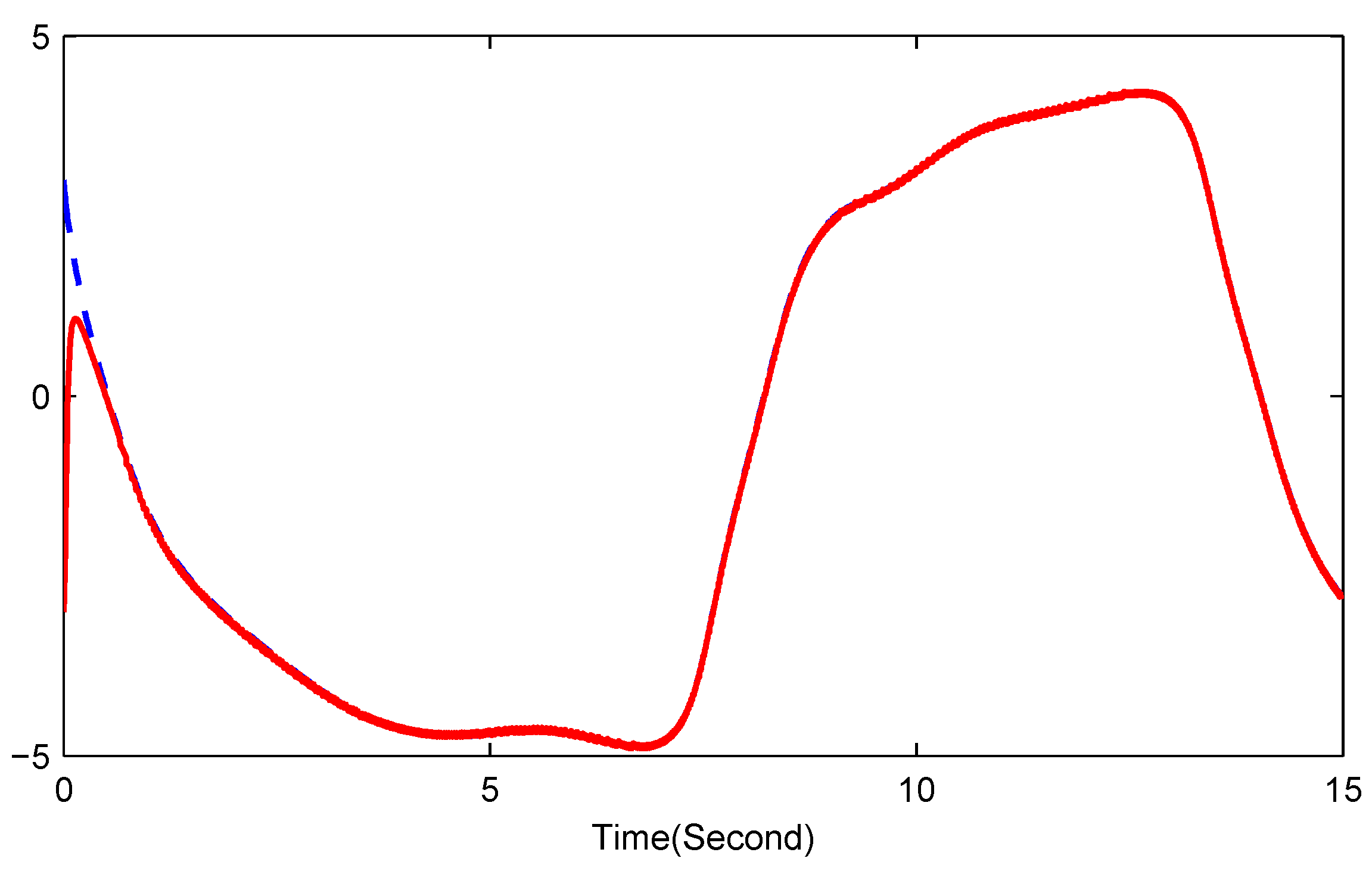
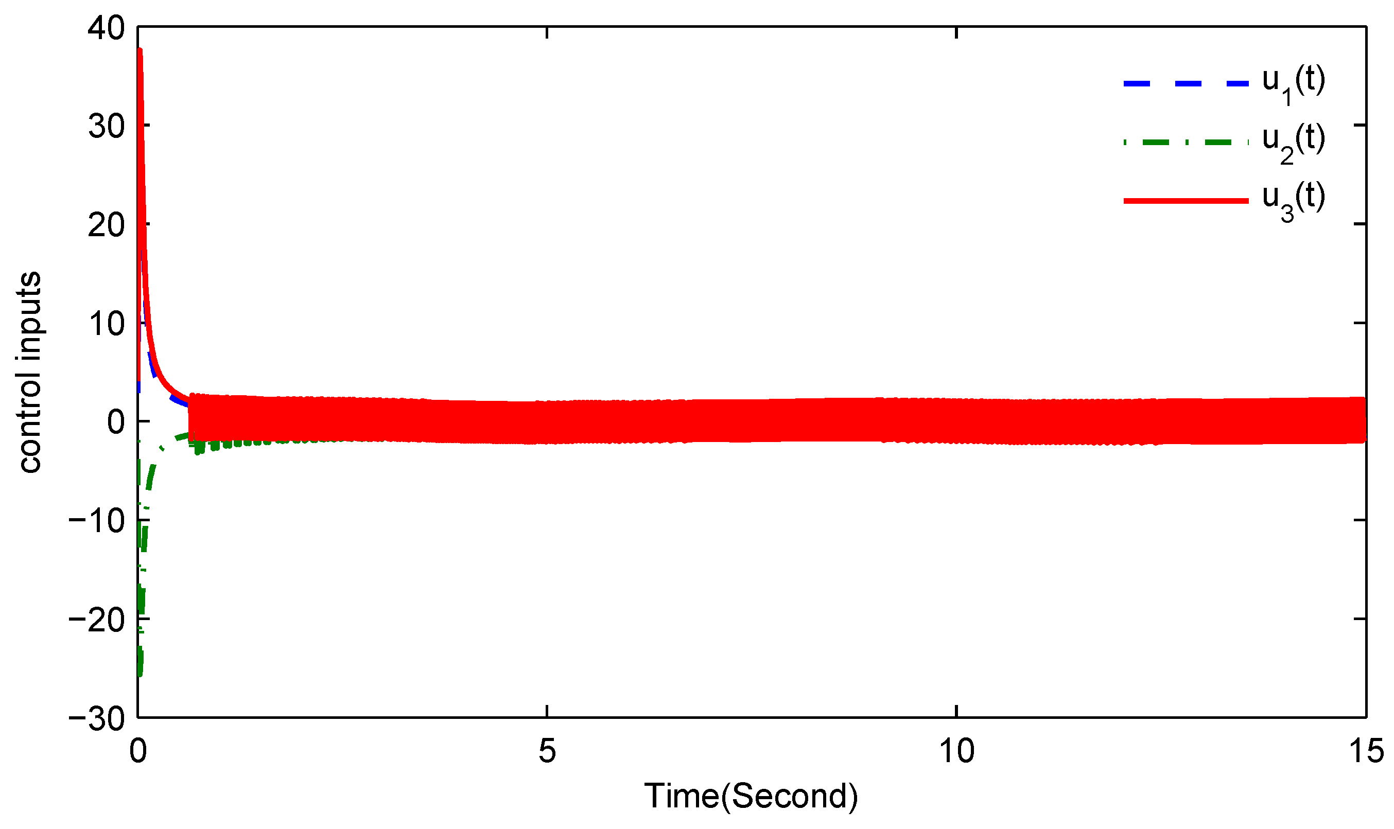
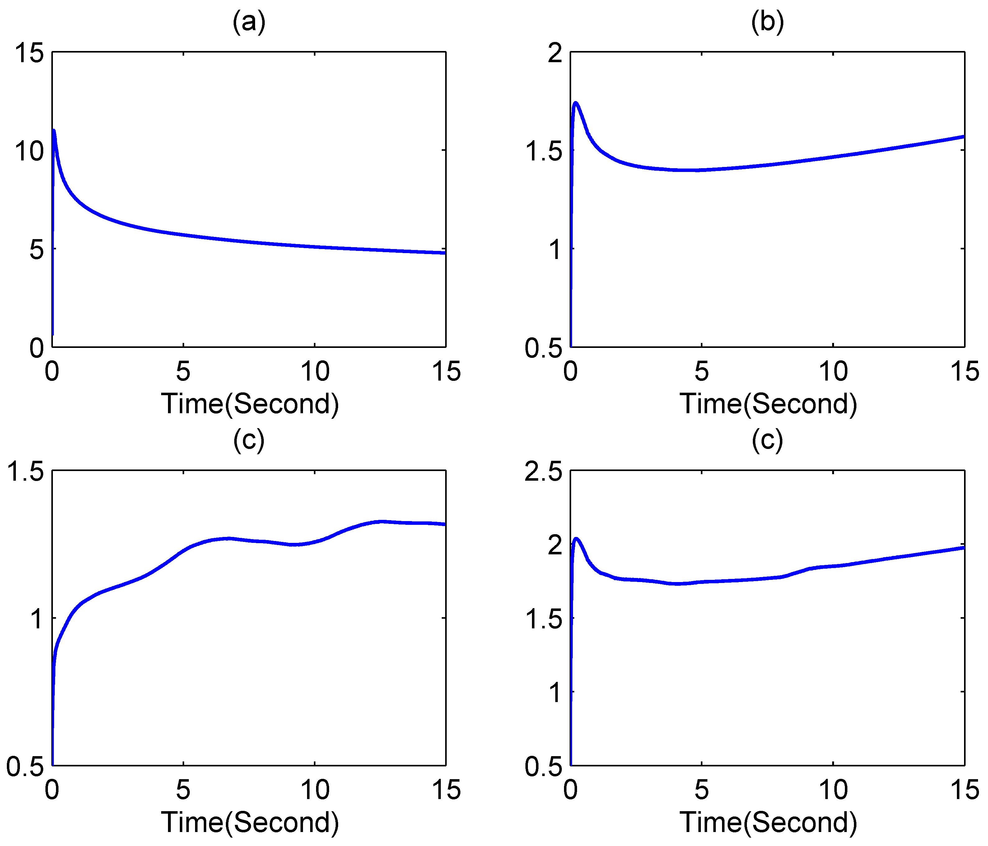
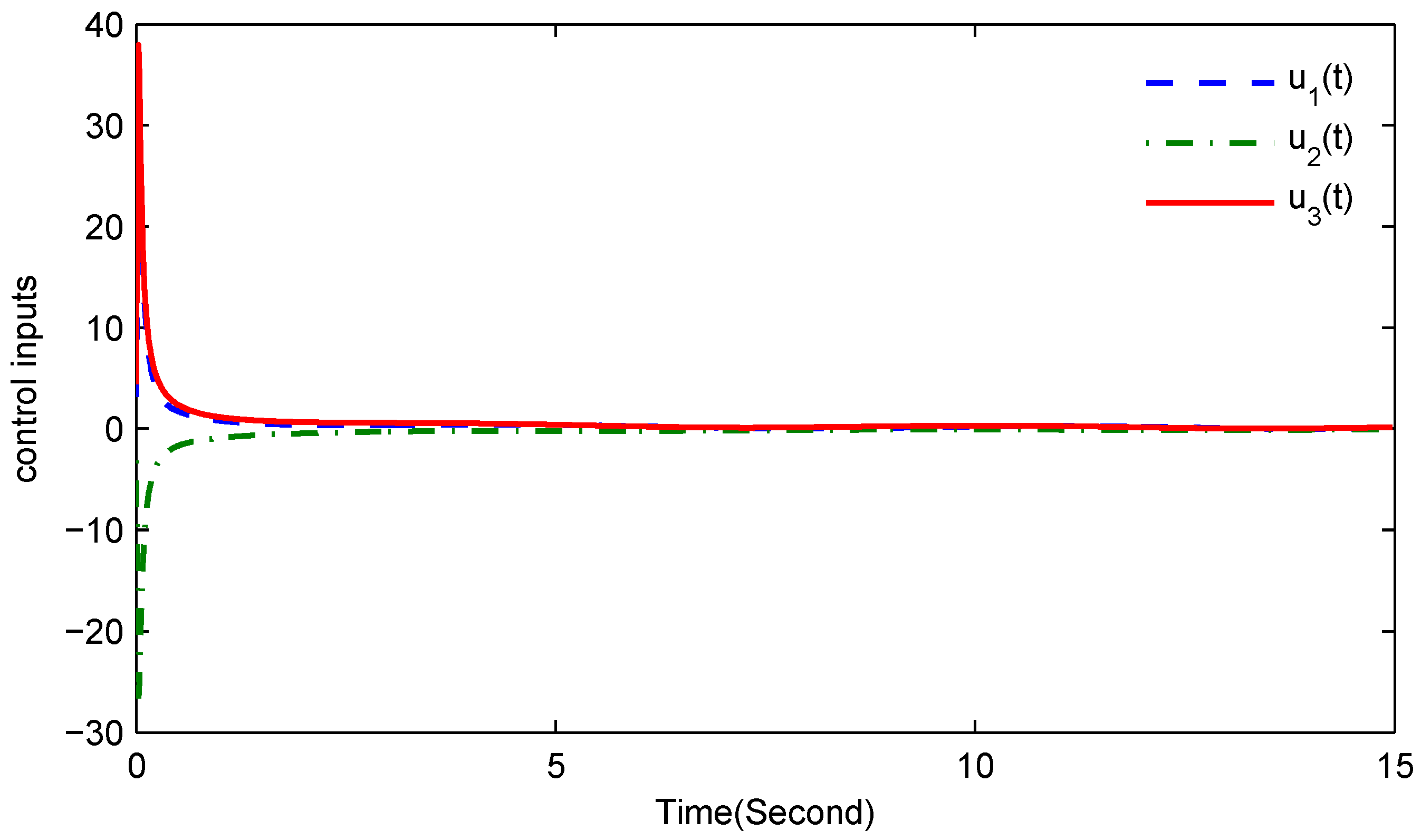
4. Simulation Studies

In the drive neural network (15), let the fractional order α be α = 0 . 81 , the nonlinear function f i ( x i ( t ) ) = tanh ( x i ( t ) ) , c i = 1 , I i = 0 for i = 1 , 2 , 3 , and A ¯ = 2 + sin t 1 . 20 2 sin t 1 . 80 1 . 71 + cos t 1 . 15 4 . 75 sin t 1 . 10 .
Under these parameters, the dynamical behavior of neural network (15) is depicted in Figure 1.
Figure 1. Dynamical behavior of system (15) with initial value [ 2 , 2 , 3 ] T .
Entropy 17 07185 g001
With respect to the response neural network (18), the initial values are chosen as y 1 ( 0 ) = 2 , y 2 ( 0 ) = 2 , y 3 ( 0 ) = 3 . The design parameters are chosen as σ = 2 , γ 1 = γ 3 = 3 , γ 2 = 1 . The external disturbance is chosen as d ( t ) = [ 0 . 5 sin ( t ) , 0 . 4 cos ( t ) , 0 . 2 sin ( t ) + 0 . 2 cos ( t ) ] T , and we can see that Assumption 3 is satisfied. Besides, we can see that the controller has nothing to to with the systems nonlinear functions f ( x ( t ) ) and f ( y ( t ) ) once Assumption 1 is satisfied. Here we give the exact models of the two fractional-order neural networks is only for the simulation purpose.
The simulation results are depicted in Figure 2, Figure 3, Figure 4, Figure 5, Figure 6 and Figure 7. Figure 2, Figure 3, Figure 4 and Figure 5 show the synchronization between two fractional-order neural networks and the time response of the synchronization errors. The time response of the the control inputs, and the updated parameters are included in Figure 6 and Figure 7, respectively. From the results we can see that the synchronization errors converge to origin rapidly, and favorable synchronization performance has been achieved.
Figure 2. Synchronization between x 1 ( t ) (dashed line) and y 1 ( t ) (solid line).
Entropy 17 07185 g002
Figure 3. Synchronization between x 2 ( t ) (dashed line) and y 2 ( t ) (solid line).
Entropy 17 07185 g003
Figure 4. Synchronization between x 3 ( t ) (dashed line) and y 3 ( t ) (solid line).
Entropy 17 07185 g004
Figure 5. Synchronization errors.
Entropy 17 07185 g005
Figure 6. Control inputs.
Entropy 17 07185 g006
Figure 7. The time response of control parameters: (a) a ^ ( t ) , (b) ρ ^ 1 ( t ) , (c) ρ ^ 2 ( t ) , (d) ρ ^ 3 ( t ) .
Entropy 17 07185 g007
To avoid the chattering phenomenon which is brought form the sign function (see, the controller (23)), the sign function can be replaced by some continuous functions. For example, let us use arctan ( 20 · ) to replace sign ( · ) , the simulation results are presented in Figure 8 and Figure 9.
Figure 8. Synchronization errors without chattering phenomenon.
Entropy 17 07185 g008
Figure 9. Control inputs without chattering phenomenon.
Entropy 17 07185 g009

5. Conclusions

We investigate the robust adaptive synchronization for fractional-order neural networks with both system uncertainties and unknown Lipschitz constants. It is showed that fractional-order differential equations can be used to update parameters online and quadratic Lyapunov functions can be used in the stability analysis of fractional-order neural networks. The proposed methods enable us to establish a fundamental stability analysis framework in fractional-order neural networks. Working towards relaxing the requirements of the knowledge of system uncertainties (for example, the system uncertainties are fully unknown) in the controller design is our further investigation direction.

Acknowledgements

This research is supported by the National Natural Science Foundation of China (Grant Nos. 11401243, 61403157), the Natural Science Foundation for the Higher Education Institutions of Anhui Province of China (Grant Nos. KJ2015A178, KJ2015A256), the Jiangsu Planned Projects for Postdoctoral Research Funds (Grant No. 1501048B), the Natural Science Foundation of Anhui Province (Grant No. 1508085QA16), and the the Fundamental Research Funds for the Central Universities of China (Grant No. GK201504002).

Author Contributions

In this paper, Shenggang Li is in charge of the adaptive synchronization controller design. Heng Liu is in charge of the fractional calculus theory, the fractional-order adaptation law design and paper writing. Hongxing Wang and Yuhong Huo mainly contribute in the stability analysis, and Junhai Luo is in charge of the discussion and the simulation. All authors have read and approved the final manuscript.

Conflicts of Interest

The authors declare no conflict of interest.

References

  1. Podlubny, I. Fractional Differential Equations; Academic Press: San Diego, CA, USA, 1999. [Google Scholar]
  2. Hilfer, R. Applications of Fractional Calculus in Physics; World Scientific York: Singapore, Singapore, 2000. [Google Scholar]
  3. Chen, L.; Qu, J.; Chai, Y.; Wu, R.; Qi, G. Synchronization of a class of fractional-order chaotic neural networks. Entropy 2013, 15, 3265–3276. [Google Scholar] [CrossRef]
  4. Li, Y.; Chen, Y.; Podlubny, I. Mittag-Leffler stability of fractional order nonlinear dynamic systems. Automatica 2009, 45, 1965–1969. [Google Scholar] [CrossRef]
  5. Delavari, H.; Baleanu, D.; Sadati, J. Stability analysis of Caputo fractional-order nonlinear systems revisited. Nonlinear Dyn. 2012, 67, 2433–2439. [Google Scholar] [CrossRef]
  6. Liu, H.; Li, S.; Sun, Y.; Wang, H. Adaptive fuzzy synchronization for uncertain fractional-order chaotic systems with unknown non-symmetrical control gain. Acta Phys. Sin. 2015, 64, 070503. (In Chinese) [Google Scholar]
  7. Liu, H.; Li, S.; Sun, Y.; Wang, H. Prescribed performance synchronization for fractional-order chaotic systems. Chin. Phys. B 2015, 24, 090505. [Google Scholar] [CrossRef]
  8. Dadras, S.; Momeni, H.R. Fractional-order dynamic output feedback sliding mode control design for robust stabilization of uncertain fractional-order nonlinear systems. Asian J. Control 2014, 16, 489–497. [Google Scholar] [CrossRef]
  9. Shen, J.; Lam, J. Non-existence of finite-time stable equilibria in fractional-order nonlinear systems. Automatica 2014, 50, 547–551. [Google Scholar] [CrossRef]
  10. Yin, C.; Cheng, Y.; Zhong, S.M.; Bai, Z. Fractional-order switching type control law design for adaptive sliding mode technique of 3D fractional-order nonlinear systems. Complexity 2015. [Google Scholar] [CrossRef]
  11. Arena, P.; Caponetto, R.; Fortuna, L.; Porto, D. Bifurcation and chaos in non-integer order cellular neural networks. Int. J. Bifurac. Chaos 1998, 8, 1527–1539. [Google Scholar] [CrossRef]
  12. Petráč, I. A note on the fractional-order cellular neura lnetworks. In Proccedings of 2006 International Joint Conference on Neural Networks, Vancouver, BC, Canada, 16–21 July 2006; pp. 1021–1024.
  13. Wu, R.; Lu, Y.; Chen, L. Finite-time stability of fractional delayed neural networks. Neurocomputing 2015, 149, 700–707. [Google Scholar] [CrossRef]
  14. Huang, H.; Huang, T.; Chen, X. A mode-dependen tapproach to state estimation of recurrent neural networks with Markovian jumping parameters and mixed delays. Neural Netw. 2013, 46, 50–61. [Google Scholar] [CrossRef] [PubMed]
  15. Ma, W.; Li, C.; Wu, Y.; Wu, Y. Adaptive synchronization of fractional neural networks with unknown parameters and time delays. Entropy 2014, 16, 6286–6299. [Google Scholar] [CrossRef]
  16. Li, T.; Song, A.G.; Fei, S.M.; Guo, Y.Q. Synchronization control of chaotic neural networks with time-varying and distributed delays. Nonlinear Anal. Theory Methods Appl. 2009, 71, 2372–2384. [Google Scholar] [CrossRef]
  17. Gan, Q.T.; Hu, R.X.; Liang, Y.H. Adaptive synchronization for stochastic competitive neural networks with mixed time-varying delays. Commun. Nonlinear Sci. Numer. Simul. 2012, 17, 3708–3718. [Google Scholar] [CrossRef]
  18. Arena, P.; Fortuna, L.; Porto, D. Chaotic behavior in noninteger-order cellular neural networks. Phys. Rev. E 2000, 61, 776–781. [Google Scholar] [CrossRef]
  19. Arena, P.; Caponetto, R.; Fortuna, L.; Porto, D. Bifurcation and chaos in noninteger order cellular neural networks. Int. J. Bifurac. Chaos 1998, 8, 1527–1539. [Google Scholar] [CrossRef]
  20. Boroomand, A.; Menhaj, M. Fractional-order hopfield neural networks. In Advances in Neuro-Information Processing; Springer: Berlin/Heidelberg, Germany, 2009; pp. 883–890. [Google Scholar]
  21. Huang, X.; Zhao, Z.; Wang, Z.; Lia, Y.X. Chaos and hyperchaos in fractional-order cellular neural networks. Neurocomputing 2012, 94, 13–21. [Google Scholar] [CrossRef]
  22. Hu, C.; Yu, J.; Jiang, H. Finite-time synchronization of delayed neural networks with Cohen-Grossberg type based on delayed feed back control. Neurocomputing 2015, 143, 90–96. [Google Scholar] [CrossRef]
  23. Chen, J.; Zeng, Z.; Jiang, P. Global Mittag-Leffler stability and synchronization of memristor-based fractional-order neural networks. Neural Netw. 2014, 51, 1–8. [Google Scholar] [CrossRef] [PubMed]
  24. Bao, H.; Cao, J. Projective synchronization of fractional-order memristor-based neural networks. Neural Netw. 2015, 63, 1–9. [Google Scholar] [CrossRef] [PubMed]
  25. Aguila-Camacho, N.; Duarte-Mermoud, M.A.; Gallegos, J.A. Lyapunov functions for fractional order systems. Commun. Nonlinear Sci. Numer. Simul. 2014, 19, 2951–2957. [Google Scholar] [CrossRef]
  26. Duarte-Mermoud, M.A.; Aguila-Camacho, N.; Gallegos, J.A.; Castro-Linares, R. Using general quadratic Lyapunov functions to prove Lyapunov uniform stability for fractional order systems. Commun. Nonlinear Sci. Numer. Simul. 2015, 22, 650–659. [Google Scholar] [CrossRef]
  27. Lazarević, M.P.; Debeljković, D.L. Finite time stability analysis of linear autonomous fractional order systems with delayed state. Asian J. Control 2005, 7, 440–447. [Google Scholar]
  28. Asheghan, M.M.; Delshad, S.S.; Beheshti, M.T.H.; Tavazoei, M.S. Non-fragile control and synchronization of a new fractional order chaotic system. Appl. Math. Comput. 2013, 222, 712–721. [Google Scholar] [CrossRef]
  29. Yu, J.; Hu, C.; Jiang, H. α-stability and α-synchronization for fractional-order neural networks. Neural Netw. 2012, 35, 82–87. [Google Scholar] [CrossRef] [PubMed]
  30. Li, K.; Peng, J.; Gao, J. A comment on “α-stability and α-synchronization for fractional-order neural networks”. Neural Netw. 2013, 48, 207–208. [Google Scholar]

