The Bogdanov–Takens Normal Form: A Minimal Model for Single Neuron Dynamics

Abstract

Conductance-based (CB) models are a class of high dimensional dynamical systems derived from biophysical principles to describe in detail the electrical dynamics of single neurons. Despite the high dimensionality of these models, the dynamics observed for realistic parameter values is generically planar and can be minimally described by two equations. In this work, we derive the conditions to have a Bogdanov–Takens (BT) bifurcation in CB models, and we argue that it is plausible that these conditions are verified for experimentally-sensible values of the parameters. We show numerically that the cubic BT normal form, a two-variable dynamical system, exhibits all of the diversity of bifurcations generically observed in single neuron models. We show that the Morris–Lecar model is approximately equivalent to the cubic Bogdanov–Takens normal form for realistic values of parameters. Furthermore, we explicitly calculate the quadratic coefficient of the BT normal form for a generic CB model, obtaining that by constraining the theoretical I-V curve’s curvature to match experimental observations, the normal form appears to be naturally cubic. We propose the cubic BT normal form as a robust minimal model for single neuron dynamics that can be derived from biophysically-realistic CB models.

1. Introduction

Our purpose here is to present a robust minimal model for single neuron dynamics. We have a dynamical systems approach, and the detailed calculations can be found in [1].

Near a bifurcation, the behavior of any physical system is universal (i.e., not dependent on its specific details) and is described by a universal equation called the normal form [2,3]. These equations are universality classes, and very different dynamical systems (near a given bifurcation) will be described by the same normal form. Although this is mathematically strictly true infinitesimally near the bifurcation, it occurs often that the qualitative aspects of the behavior of the system are still given by the normal form, even outside of the infinitesimal neighborhood of the bifurcation point. In this work, we will show that the electrical dynamics of a single neuron can be an example of this fact.

At the present time, to describe neuronal dynamics for different types of neurons, there is an overwhelming diversity of thousands of high dimensional nonlinear models. This class of models is called conductance-based models (CB models), and they are considered the most biophysically realistic models [4,5,6,7]. In the last few decades, the detailed electrophysiological and biophysical description of the wide diversity of conductances [8] led scientists to the possibility of building a detailed CB model of many of the neuronal types studied [5]. Each different CB model, built using adjustments of parameters with the experimental data, can have more than twenty nonlinear equations. This has generated in the last few decades a massive production of different CB models for different types of neurons or experimental scenarios and the development of databases of thousands of different CB models [9].

Although there is a huge diversity of types of neurons (and CB models), there is a robust dynamics observed experimentally (and numerically) in almost all of them. This distinctive electrical dynamics observed in neurons is called the excitable behavior of neurons. In 1948, it was Hodgkin who classified this excitable behavior observed in neurons into two major groups [10]: (1) Class I neural excitability: action potentials can be generated with arbitrarily low frequency, depending on the strength of the applied current; (2) Class II neural excitability: action potentials are generated in a certain frequency band that is relatively insensitive to changes in the strength of the applied current.

In the late 1990s, a connection between this classification and bifurcation theory was noticed [11]. It was realized that Class I neural excitability is consistent with a saddle-node homoclinic bifurcation. On the other hand, Class II neural excitability was consistent with a local subcritical Andronov–Hopf bifurcation with a narrow range of bistability. However, it has been shown that this classification is consistent with a broader set of global bifurcation, such as saddle-node homoclinic bifurcation, the saddle-homoclinic bifurcation and the big homoclinic bifurcation, which can lead to secondary local bifurcations. Therefore, despite the huge diversity of types of neurons and models, they display a universal dynamics generically captured by a two-variable dynamical system [7,12,13]. These minimal models can be phenomenological models or reduced CB models. Procedures have been developed to reduce the number of variables in CB models [7,14]. However, the mathematical mechanisms by which single neurons display this universal planar dynamics are still not fully clear.

We propose here a solution to this problem adopting a dynamical systems approach, with the idea that we have to look for a robust behavior related to the experimental data and construct from its analysis the simplest possible model satisfying the requirements.

We first show that due to the very special mathematical structure of CB models if we impose the conditions to have in some neighborhood of the space of parameters both the saddle-node and the Andronov–Hopf bifurcations, we naturally arrive at the Bogdanov–Takens (BT) bifurcation point. Furthermore, we find that these conditions are equivalent to having both positive and negative feedback and a time scale separation, which are precisely two conditions that have been reported as a key dynamical mechanism for neurons to exhibit excitable behavior [15,16]. However, we still have to impose that the system should be in the neighborhood of the transition between having one or three fixed points, since both situations are generically observed experimentally [7]. We show that this last requirement is satisfied imposing a third condition, which implies that the coefficient of a quadratic term in the BT normal form at the critical point vanishes. We have then to include cubic nonlinearities at the critical point, and the quadratic term will appear with a small coefficient as an unfolding term (as happens in a subcritical bifurcation). The calculation of the cubic BT normal form gives us explicit formulas for the coefficients in terms of the parameters of the CB model under consideration. Additionally, all of the original variables of the CB model are expressed in terms of the critical variables, which we can choose to be $(u,\dot{u})$, where u is the membrane potential and $\dot{u}$ its time derivative. The coefficients and the original physical variables are given by analytical expressions, which result from a standard calculation using the results in [1,17,18]. We present here the BT cubic normal form in Arnold’s choice, which leads to a second order in the time differential equation for the variable u, which has a very appealing mechanical interpretation as a Hamiltonian system with a nonlinear friction. We investigate numerically this equation, and we find that it robustly exhibits the local and global bifurcations observed in single neurons.

2. Conductance-Based Models

2.1. Mathematical Structure of Conductance-Based Models

CB models are a class of ODEs with a special structure that can be completely characterized. In any CB model, there is one variable that in this paper we will call u that represents the membrane potential and other set of variables that we will call $m_j$ that represents the gating probability of a ion channel sub-unit over time. In nondimensional variables, a general form of a CB model can be written as follows:

$$\begin{array}{c}\hfill \begin{array}{cc}\hfill \dot{u}& =I-I_{\text{ionic}}(u,\overrightarrow{m};\overrightarrow{\eta })\hfill \\ \hfill \dot{m_j}& =\frac{m_j^{\infty }(u;{\overrightarrow{\sigma }}_j)-m_j}{{\tau }_j(u;{\overrightarrow{\sigma }}_j)}j=1,2\cdots N\hfill \end{array}\end{array}$$

(1)

The functions $m_j^{\infty }(u;{\overrightarrow{\sigma }}_j)$ represent the stationary probability of a gating variable $m_j$ to be activated, and ${\tau }_j(u;{\overrightarrow{\sigma }}_j)$ is its decay time. Typically, $m_j^{\infty }(u;{\overrightarrow{\sigma }}_j)$ and ${\tau }_j(u;{\overrightarrow{\sigma }}_j)$ are functions of the membrane potential u and depend on the same set of parameters ${\overrightarrow{\sigma }}_j$. These parameters are shaped by the biophysical structure of the ion channel and its kinetic properties. We will call the vector formed by the union of all these parameters ${\overrightarrow{\sigma }}_T$ (i.e., ${\overrightarrow{\sigma }}_T={\cup }_{j=1}^k{\overrightarrow{\sigma }}_j$). The symbol I represents the input current to the neuron, and the function $I_{\text{ionic}}(u,\overrightarrow{m};\overrightarrow{\eta })$ represents the overall ionic current that goes through the membrane. This last quantity depends on parameters, such as the reversal potential and the maximal conductance of a specific ionic current. We will use the vector $\overrightarrow{\eta }$ to collect together all of these parameters of different ion channels (i.e., $\overrightarrow{\eta }=\left(u_1,\cdots ,u_n,g_1\cdots ,g_n\right)$). In general, for any conductance-based model, the overall ionic current can be written as follows:

$$I^{\text{ionic}}(u,\overrightarrow{m};\overrightarrow{\eta })\equiv \sum _{j=1}^n{I}_j^{\text{ionic}}=\sum _{j=1}^n{g}_j\prod _{l\in w_j}{m}_l^{p_l}(u-u_j)$$

(2)

Each $I_j^{\text{ionic}}$ represents an ionic current associated with an ionic conductance j (or ion channel j) and, in general, can be written as:

$$I_j^{\text{ionic}}=g_j\prod _{l\in w_j}{m}_l^{p_l}(u-u_j)$$

(3)

where $g_j$ is the maximal conductance and $u_j$ is the reversal potential associated with the j-th ionic current. For a given current $I_j^{\text{ionic}}$, there is a specific set of gating variables ($\left\{m_l:l\in w_j\right\}$) that dynamically controls the current (see Equation (3)). We will define $w_j$ as the set of indexes that represents the identities of the gating variables present in a given ionic current j (e.g., for the Hodgkin and Huxley model, the sodium current has the gating variables m and h). Because each gating variable $m_l$ represents the probability of a specific sub-unit of a given ionic channel j to be open, the same gating variable cannot belong to two different ionic currents. This restriction is based on the nature of the ionic channel’s biophysics: the activity of one ionic channel does not directly affect the activity of another ionic channel (indirectly, it does through the coupling with the potential u), since their mechanisms of opening and closing are not physically connected [19]. Then, all of the sets of indexes $w_j$ are disjoint.

2.2. The Linear Part Is a Rank-1 Updated Diagonal Matrix

By doing the following nonsingular translation $\overrightarrow{m}={\overrightarrow{m}}^{\infty }(u;\overrightarrow{\sigma })+\overrightarrow{x}$, any generic CB model equation (i.e., Equation (1)) can be transformed into the equivalent equation:

$$\begin{array}{ccc}& \dot{u}& =I-I^{\text{ionic}}(u,{\overrightarrow{m}}^{\infty }+\overrightarrow{x};\overrightarrow{\eta })\hfill \end{array}$$

$$\begin{array}{ccc}& \dot{x_j}& =-\frac{x_j}{{\tau }_j(u;{\overrightarrow{\sigma }}_j)}-\frac{\partial m_j^{\infty }(u;{\overrightarrow{\sigma }}_j)}{\partial u}\dot{u}j=1,2,\cdots ,N\hfill \end{array}$$

(4)

Using Definition (2), the total ionic current reads:

$$I^{\text{ionic}}(u,{\overrightarrow{m}}^{\infty }(u;{\overrightarrow{\sigma }}_T)+\overrightarrow{x};\overrightarrow{\eta })=\sum _{j=1}^n{g}_j\prod _{l\in w_j}\sum _{k_l=0}^{p_l}\left(\genfrac{}{}{0pt}{}{p_l}{k_l}\right)x_l^{p_l-k_l}{\left[m_l{(u;{\overrightarrow{\sigma }}_l)}^{\infty }\right]}^{k_l}(u-u_j)$$

(5)

If we consider long times, such that all of the gating variables have relaxed ($\overrightarrow{x}=\overrightarrow{0}$), the ionic current written as (5) becomes the well-known stationary I-V curve widely used in electrophysiological studies [16,19]. We will call the stationary ionic current $I^{\infty }(u;{\overrightarrow{\sigma }}_T,\overrightarrow{\eta })$ the I-V curve of our model. It is important to notice that this function depends only on the membrane potential (u) and the sets of parameters ${\overrightarrow{\sigma }}_T$ and $\overrightarrow{\eta }$, but not the gating variables ($\overrightarrow{x}$). The stationary ionic current is given by:

$$I^{\infty }(u;{\overrightarrow{\sigma }}_T,\overrightarrow{\eta })\equiv \sum _{j=1}^n{g}_j\prod _{l\in w^{\left(j\right)}}{\left[m_l{(u;{\overrightarrow{\sigma }}_l)}^{\infty }\right]}^{p_l}(u-u_j)$$

(6)

We will define the transient current as $I^{\text{T}}(u,\overrightarrow{x};{\overrightarrow{\sigma }}_T)$, as the part of the total current that depends on both u and $\overrightarrow{x}$ and disappears for long times, such that all of the gating variables have relaxed, i.e.:

$$I^{\text{T}}(u,\overrightarrow{x};{\overrightarrow{\sigma }}_T,\overrightarrow{\eta })\equiv I^{\text{ionic}}(u,\overrightarrow{x};{\overrightarrow{\sigma }}_T,\overrightarrow{\eta })-I^{\infty }(u;{\overrightarrow{\sigma }}_T,\overrightarrow{\eta })$$

(7)

Note that $I^{\text{T}}(u,\overrightarrow{x};{\overrightarrow{\sigma }}_T,\overrightarrow{\eta })$ is at least linearly proportional to any of the variables $x_j$. This means that when all of the gating variables decay to the stationary value (i.e., $m=m^{\infty }(u;{\overrightarrow{\sigma }}_j)$), then the transient current is zero $I^{\text{T}}(u,\overrightarrow{x};{\overrightarrow{\sigma }}_T,\overrightarrow{\eta })=0$, which is the definition of a variable that acts transiently in this context. Now, we will define:

$${\beta }_j(u;{\overrightarrow{\sigma }}_j)\equiv -\frac{\partial m_j^{\infty }(u;{\overrightarrow{\sigma }}_j)}{\partial u}$$

(8)

Note that due to the form of $m_j^{\infty }(u;{\overrightarrow{\sigma }}_j)$, which is a strictly increasing (or decreasing) function of u, one has that ${\beta }_j(u;{\overrightarrow{\sigma }}_j)$ is strictly negative (or positive). Then, any CB model can be re-written in the following form:

$$\begin{array}{c}\hfill \begin{array}{cc}\hfill \dot{u}& =I-I^{\infty }(u;{\overrightarrow{\sigma }}_T,\overrightarrow{\eta })-I^T(u,\overrightarrow{x};{\overrightarrow{\sigma }}_T,\overrightarrow{\eta })\hfill \\ \hfill \dot{x_j}& =-\frac{x_j}{{\tau }_j(u;{\overrightarrow{\sigma }}_j)}+{\beta }_j(u;{\overrightarrow{\sigma }}_j)\dot{u}j=1,2\cdots N\hfill \end{array}\end{array}$$

(9)

The dynamics of each gating variable $m_j$ is a linear decay to its stationary value (which corresponds to $x_j=0$) plus a perturbation driven by the difference between the input current and the ionic current and weighted by the derivative of their corresponding stationary gating variable function. The conditions to have a fixed point are:

$$\begin{array}{c}\hfill \begin{array}{cc}\hfill I& =I^{\infty }(u^{*};{\overrightarrow{\sigma }}_T,\overrightarrow{\eta })\hfill \\ \hfill \overrightarrow{x}& =\overrightarrow{0}\hfill \end{array}\end{array}$$

(10)

A fixed point occurs when all of the gating variables have relaxed to their stationary value (i.e., $m_j=m_j^{\infty }(u;{\overrightarrow{\sigma }}_k)$) and when there is no net flux of current through the neuron membrane. The fixed points must satisfy $\overrightarrow{x}=0$ and $I=I^{\infty }(u;{\overrightarrow{\sigma }}_T,\overrightarrow{\eta })$. This equation has at least one root, since the function $I^{\infty }(u;{\overrightarrow{\sigma }}_T,\overrightarrow{\eta })$ for $u\to \pm \infty$ can only have a non-negative and constant slope (because the conductances $g_j$ are always positive quantities), but generically has one or three [4,6,7]. Then, the existence or disappearance of fixed points in this $N+1$ dimensional dynamical system depends on a one-dimensional equation $I=I^{\infty }(u;{\overrightarrow{\sigma }}_T,\overrightarrow{\eta })$. We can choose a root $u^{*}$ of this equation as a continuous parameter of bifurcation instead of the parameter I, which is the one that is experimentally tuned, as long as we stay in the same branch of the equation. Thus, by doing the standard translations in the neighborhood of the fixed point ($\overrightarrow{x}=\overrightarrow{0}+\delta \overrightarrow{x}$ and $u=u^{*}+\delta u$) and after some algebra using Equation (9), we find that the linear matrix has the form:

$$\mathbb{L}(u^{*};{\overrightarrow{\sigma }}_T,\overrightarrow{\eta })=\mathbb{A}(u^{*};{\overrightarrow{\sigma }}_T)+\overrightarrow{\beta }(u^{*};{\overrightarrow{\sigma }}_T,\overrightarrow{\eta }){\overrightarrow{M}}^T(u^{*};{\overrightarrow{\sigma }}_T,\overrightarrow{\eta })$$

(11)

where:

$${\mathbb{A}}_{i,j}(u^{*};{\overrightarrow{\sigma }}_T)=\left\{\begin{array}{cc}0\hfill & \text{if }i\ne j\text{or }i=j=0\hfill \\ -\frac{1}{{\tau }_i(u^{*},{\overrightarrow{\sigma }}_i)}\hfill & \text{if }i=j\hfill \end{array}\right.$$

(12)

and:

$$M_i(u^{*};{\overrightarrow{\sigma }}_T,\overrightarrow{\eta })=\left\{\begin{array}{cc}-{\left.\frac{\partial I^{\infty }(u;{\overrightarrow{\sigma }}_T,\overrightarrow{\eta })}{\partial u}\right|}_{u=u^{*}}\hfill & \text{if }i=0\hfill \\ -{\left.\frac{\partial I^T(u,\overrightarrow{x};{\overrightarrow{\sigma }}_T,\overrightarrow{\eta })}{\partial x_i}\right|}_{u=u^{*},x_i=0}\hfill & \text{if }i=1,\cdots ,N\hfill \end{array}\right.$$

(13)

and:

$${\beta }_i(u^{*};{\overrightarrow{\sigma }}_i)=\left\{\begin{array}{cc}1\hfill & \text{if }i=0\hfill \\ -{\left.\frac{\partial m_i^{\infty }(u;{\overrightarrow{\sigma }}_i)}{\partial u}\right|}_{u=u^{*}}\hfill & \text{if }i=1,\cdots ,N\hfill \end{array}\right.$$

(14)

The structure of the matrix in (11) is known as a rank-1 updated matrix. As the name states, the matrix $\mathbb{L}$ is the sum of the diagonal matrix $\mathbb{A}$ plus a rank-1 perturbation, which corresponds to $\overrightarrow{\beta }{\overrightarrow{M}}^T$. We will use this fact to provide a closed form to the characteristic polynomial of the linear approximation for CB models. For simplicity, throughout the rest of the text, we will not write explicitly the dependence on the parameters ${\overrightarrow{\sigma }}_T$ and $\overrightarrow{\eta }$.

2.3. Characteristic Polynomial

Using known expressions [20,21] for the determinant of a rank-1 updated matrix, we have that the characteristic polynomial of any conductance-based model can be written as:

$$P_N\left(\lambda \right)=\text{Det}\left(\mathbb{A}-\lambda \mathbb{I}\right)\left(1+{\overrightarrow{M}}^T{\left(\mathbb{A}-\lambda \mathbb{I}\right)}^{-1}\overrightarrow{\beta }\right)$$

Providing that $\lambda \ne -1/{\tau }_j\forall j$, which is equivalent to:

$$P_N\left(\lambda \right)={(-1)}^N\left\{{\beta }_0{M}_0\prod _{l=1}^N\left(\frac{1}{{\tau }_l}+\lambda \right)-\lambda \left[\prod _{j=1}^N\left({\frac{1}{\tau }}_j+\lambda \right)-\sum _{s=1}^N{\beta }_s{M}_s\prod _{l\ne s}^N\left(\frac{1}{{\tau }_l}+\lambda \right)\right]\right\}$$

(15)

The last expression is the general form for the characteristic polynomial of any conductance-based model. Then, this expression can be used to find analytic formulas for local bifurcations. To our knowledge, this is the first time that an analytic expression is given for the characteristic polynomial of a conductance-based model with an arbitrary number of conductances. For simplicity, in this section, we did not include explicitly the dependence on the fixed point $u^{*}$.

3. Cubic Bogdanov–Takens Normal Form in Conductance-Based Models

3.1. Bogdanov–Takens Bifurcation in Conductance-Based Models

We are looking for a critical point that encloses most of the diverse, but planar (two variables) dynamics observed in single neurons. In electrophysiological experiments, when the transmembrane current I is increased, neuron dynamics abruptly transit from a fixed point (rest potential) to a limit cycle (spiking). This transition to relaxation oscillations is the landmark of single neuron dynamics. Often, different classes of neurons have different types of spiking dynamics. The rest potential can exhibit an exponential decay after being perturbed (node) or damped oscillations (focus). In addition, the transition to spiking can occur via many dynamical mechanisms as saddle-node homoclinic bifurcation, bistability between a focus and limit cycle, subcritical Andronov–Hopf bifurcation between others. These dynamical mechanisms are seldom controlled by the experimenter, but they depend on the specific class of neuron, that is its specific set of ionic conductances and the values of its parameters. When the current I is increased, depending on the type of neuron, the local bifurcations observed are usually saddle-node or Andronov–Hopf. Then, the first condition that we will impose for a critical point that encloses the diversity observed in single neurons dynamics is to have both local saddle-node and Andronov–Hopf bifurcation in its neighborhood. This must be a bifurcation point of at least codimension two, since we need one parameter (usually I) to reach the bifurcation and another to transit from saddle-node to Andronov–Hopf (or vice versa). We exclude the bifurcation arising from the eigenvalues $(0,+i\omega ,-i\omega )$, i.e., a simultaneous saddle-node and Andronov–Hopf bifurcation, since it leads to a three-variable dynamics. A low codimension candidate for this is a double zero bifurcation (two eigenvalues equal to zero). Slight departures in the parameter space from this point will transform this double zero in a saddle-node or an Andronov–Hopf bifurcation locally. Using the characteristic polynomial (Equation (15)), we can find analytically the conditions to have double zero eigenvalues:

$$\begin{array}{ccc}\hfill {\beta }_0\left(u^{*}\right)M_0\left(u^{*}\right)\prod _{i=1}^N\frac{1}{{\tau }_i\left(u^{*}\right)}& =& 0\hfill \\ \hfill \prod _{i=1}^N\frac{1}{{\tau }_i\left(u^{*}\right)}-\sum _{j=1}^N{\beta }_j\left(u^{*}\right)M_j\left(u^{*}\right)\prod _{l\ne j}^N\frac{1}{{\tau }_i\left(u^{*}\right)}& =& 0\hfill \end{array}$$

Since the relaxation times of the gating variables (${\tau }_i\left(u^{*}\right)$) are always positive quantities, then these two conditions are equivalent to:

$$\begin{array}{ccc}\hfill {\left.\frac{\partial I^{\infty }\left(u\right)}{\partial u}\right|}_{u=u^{*}}& =& 0\hfill \\ \hfill 1-\sum _{j=1}^N{\left.\frac{\partial m_j^{\infty }\left(u\right)}{\partial u}\right|}_{u=u^{*}}{\left.\frac{\partial I^T(u,\overrightarrow{x})}{\partial x_j}\right|}_{u=u^{*};\overrightarrow{x}=\overrightarrow{0}}{\tau }_j\left(u^{*}\right)& =& 0\hfill \end{array}$$

Using Expressions (6) and (7), we obtain that the previous expression is equivalent to:

$$\begin{array}{ccc}\hfill \sum _{j=1}^n{g}_j\prod _{l\in w^{\left(j\right)}}{\left[m_l{\left(u^{*}\right)}^{\infty }\right]}^{p_l}+\sum _{j=1}^N{\left.\frac{\partial m_j^{\infty }\left(u\right)}{\partial u}\right|}_{u=u^{*}}{\left.\frac{\partial I^T(u,\overrightarrow{x})}{\partial x_j}\right|}_{u=u^{*};\overrightarrow{x}=\overrightarrow{0}}& =& 0\hfill \\ \hfill 1-\sum _{j=1}^N{\left.\frac{\partial m_j^{\infty }\left(u\right)}{\partial u}\right|}_{u=u^{*}}{\left.\frac{\partial I^T(u,\overrightarrow{x})}{\partial x_j}\right|}_{u=u^{*};\overrightarrow{x}=\overrightarrow{0}}{\tau }_j\left(u^{*}\right)& =& 0\hfill \end{array}$$

At this point, it is necessary to define the following quantity:

$$\begin{array}{ccc}\hfill {\tau }_0\left(u^{*}\right)& \equiv & \frac{1}{{\sum }_{j=1}^n{g}_j{\prod }_{l\in w^{\left(j\right)}}{\left[m_l{\left(u^{*}\right)}^{\infty }\right]}^{p_l}}\hfill \\ \hfill G_j\left(u^{*}\right)& \equiv & {\left.\frac{\partial m_j^{\infty }\left(u\right)}{\partial u}\right|}_{u=u^{*}}{\left.\frac{\partial I^T(u,\overrightarrow{x})}{\partial x_j}\right|}_{u=u^{*};\overrightarrow{x}=\overrightarrow{0}}\hfill \end{array}$$

The function ${\tau }_0\left(u^{*}\right)$ can be interpreted as the relaxation time of the ohmic part of the I-V curve. The function $G_j\left(u^{*}\right)$, called the gating function, will quantify the linear contribution of a given gating variable j to the overall CB model dynamics. The sign of $G_j\left(u\right)$ will determine if a gating variable is an amplifier (i.e., contributes to the dynamics as a positive feedback, is negative) or resonant (i.e., contribute to the dynamics as negative feedback, is positive) according to the classification used in computational neuroscience [7]. This naturally leads us to a sign criteria to designate an amplifier or a resonant gating variable. Using these definitions, we can write the double zero condition in terms of the gating functions and relaxation times:

$$\begin{array}{ccc}\hfill 1+{\tau }_0\left(u^{*}\right)\sum _{j=1}^N{G}_j\left(u^{*}\right)& =& 0\hfill \end{array}$$

(16)

$$\begin{array}{ccc}\hfill 1-\sum _{j=1}^N{G}_j\left(u^{*}\right){\tau }_j\left(u^{*}\right)& =& 0\hfill \end{array}$$

(17)

Since the relaxation times (${\tau }_0\left(u^{*}\right)$ and ${\tau }_j\left(u^{*}\right)$) are positive quantities, then after some simple algebra, we can conclude that the necessary conditions for having a double zero bifurcation are: (1) at least one amplifier and one resonant gating variable (i.e., at least one $G_j\left(u^{*}\right)$ must have a different sign); (2) at least one gating variables relaxation time is different. In other words, a conductance-based model must have gating variables that produce both positive and negative feedback, and there must be a time scale separation between at least one of them. Furthermore, we showed that if the system has two time scales, the fastest gating variables must be an amplifier and the slower resonant (Supplementary Materials, Section 2). This result is surprising, since the conditions mentioned have been reported as a key dynamical mechanism for neurons to exhibit excitable behavior [15,16]. In addition, we showed that in CB models, a double zero bifurcation is always a BT bifurcation (Supplementary Materials, Section 1.1). Additionally, we calculated the complete Jordan base (Supplementary Materials, Section 1.2) and showed that generically, a Jordan block will arise. An example of the BT bifurcation in the widely-known Hodgkin and Huxley CB model [15] is shown in Figure 1B.

3.2. Additional Condition to the Bogdanov–Takens Bifurcation

We already identified BT as a critical point of interest. However, there is an important feature that is commonly observed in neurons and neuron models that was not included in the later discussion. It has been observed in experiments and simulations that under realistic parameter values, the I-V curve is usually either monotonically increasing or has two changes in its concavity (see Figure 1A). As we discussed in Section 2, the zeros of the I-V curve determine the fixed points of the dynamics. Then, if the I-V curve is monotonically increasing, the dynamics will have just one fixed point, and if its concavity changes just twice, it has three. Nevertheless, the stability of the fixed point depends on the eigenvalues of the linear matrix, which can be calculated using the expression for the characteristic polynomial in Equation (15), and they do not depend explicitly on the second derivative of the I-V curve. Since we want to include both scenarios (one fixed point and three fixed points) in the neighborhood of the critical point, then we need to impose that:

$$\frac{{\partial }^2{I}^{\infty }(u^{*};{\overrightarrow{\sigma }}_T,\overrightarrow{\eta })}{\partial u^2}=0$$

(18)

In addition to the two BT conditions, this third condition puts the critical point in the transition point between one to three fixed points. Then, in its neighborhood, one finds many of the local bifurcation scenarios previously observed in neuron models: Andronov–Hopf bifurcation with one fixed point, Andronov–Hopf bifurcation with three fixed points and a saddle-node with three fixed points. When the BT normal form is calculated in this point, we obtain surprising results regarding its universality to reproduce single neuron dynamics.

Figure 1. (A) The I-V curve (i.e., function $I^{\infty }\left(u^{*}\right)$) for the Hodgkin and Huxley model for three different values of the potassium conductance $g_K$. A red dot indicates a fixed point in the dynamics. (B) The Bogdanov–Takens (BT) bifurcation in the Hodgkin and Huxley model. The $1+{\tau }_0\left(u^{*}\right){\sum }_{j=1}^N{G}_j\left(u^{*}\right)$ function is shown in purple. The $1-{\sum }_{j=1}^N{G}_j\left(u^{*}\right){\tau }_j\left(u^{*}\right)$ function is shown in green. The plots in black frames show the eigenvalues of the linear matrix $\mathbb{L}\left(u^{*}\right)$ in the complex plane. We omitted the greater in absolute value eigenvalue (far to the left) in order to better visualize the two critical ones. Tags 1–3 indicate the corresponding values of the variable $u^{*}$. The plot in a red dashed frame shows the eigenvalues of the linear matrix $\mathbb{L}\left(u^{*}\right)$ in the complex plane when the model undergoes a BT bifurcation.

Figure 1. (A) The I-V curve (i.e., function $I^{\infty }\left(u^{*}\right)$) for the Hodgkin and Huxley model for three different values of the potassium conductance $g_K$. A red dot indicates a fixed point in the dynamics. (B) The Bogdanov–Takens (BT) bifurcation in the Hodgkin and Huxley model. The $1+{\tau }_0\left(u^{*}\right){\sum }_{j=1}^N{G}_j\left(u^{*}\right)$ function is shown in purple. The $1-{\sum }_{j=1}^N{G}_j\left(u^{*}\right){\tau }_j\left(u^{*}\right)$ function is shown in green. The plots in black frames show the eigenvalues of the linear matrix $\mathbb{L}\left(u^{*}\right)$ in the complex plane. We omitted the greater in absolute value eigenvalue (far to the left) in order to better visualize the two critical ones. Tags 1–3 indicate the corresponding values of the variable $u^{*}$. The plot in a red dashed frame shows the eigenvalues of the linear matrix $\mathbb{L}\left(u^{*}\right)$ in the complex plane when the model undergoes a BT bifurcation.

3.3. The Cubic Bogdanov–Takens Normal Form

Using the results in Elphick, Tirapegui, Brachet, Coullet and Iooss in [2], it is possible to characterize and calculate explicitly all of the non-linear terms for the BT normal form. In the case of the BT bifurcation, the equations obtained can be satisfied in more than one way, leaving an inherent freedom to incorporate the normal from (see Section 3, Supplementary Materials). We have two extreme choices: Arnold’s or the Takens choice [22]. Since in Arnold’s choice, we gain a Hamiltonian intuition, we make this choice here and use the Arnold form of the cubic BT normal form, which can be written as:

$$\ddot{u}=F\left(u,\alpha \right)-\dot{u}\lambda \left(u,\beta \right)$$

(19)

We will call the function $F(u,\alpha )$ the force and the function $\lambda (u,\beta )$ the friction using the obvious analogy to mechanics. More explicitly, $F\left(u,\alpha \right)=\alpha +{\gamma }_2{u}^2+{\gamma }_3{u}^3$, and $\lambda \left(u,\beta \right)=\beta +{\lambda }_{1}u+{\lambda }_2{u}^2$. The unfolding coefficients are α, β and ${\gamma }_2$. When they vanish, we are at the critical point, and when they take small values, we are in the neighborhood of the critical point, where we expect the normal form to be valid quantitatively. Outside this neighborhood, one expects a qualitative description. We have three unfolding parameters, since the codimension is three. We can define a potential $V(u,\alpha )$, such that the force $F\left(u,\alpha \right)$ is given by $F\left(u,\alpha \right)=-\frac{\partial V(u,\alpha )}{\partial u}$, where $V\left(u,\alpha \right)=-\alpha u-\frac{{\gamma }_2}{3}{u}^3-\frac{{\gamma }_3}{4}{u}^4$. Then, we can define the “energy” of the BT normal form as $E(u,\alpha )\equiv \frac{1}{2}{\dot{u}}^2+V\left(u,\alpha \right)$ and conclude that $\frac{d}{dt}E(u,\alpha )=-{\dot{u}}^2\lambda (u,\beta )$. This last equation shows that the BT normal form does not conserve the energy. The reader should notice that the BT normal form can undergo an injection or dissipation of energy depending on the sign of $\lambda (u,\beta )$, and this sign can of course change when u changes.

The most common scaling studied in the literature is quadratic, i.e., $F\left(u\right)=\alpha +{\gamma }_2{u}^2$ and $\lambda (u,\beta )=\beta +{\lambda }_{1}u$. The complete bifurcation diagram is known, and it exhibits saddle-node, Andronov–Hopf and homoclinic bifurcations [22,23]. However, the dynamics observed in this normal form is not consistent with the dynamics observed in single neurons. First, it is not bounded in the complete phase space, which means that for some regions in the phase space, u can go to infinity (see Figure 2 left plot). Second, it does not display many of the distinctive global bifurcations observed in neurons as the saddle-node homoclinic bifurcation or the saddle homoclinic bifurcation.

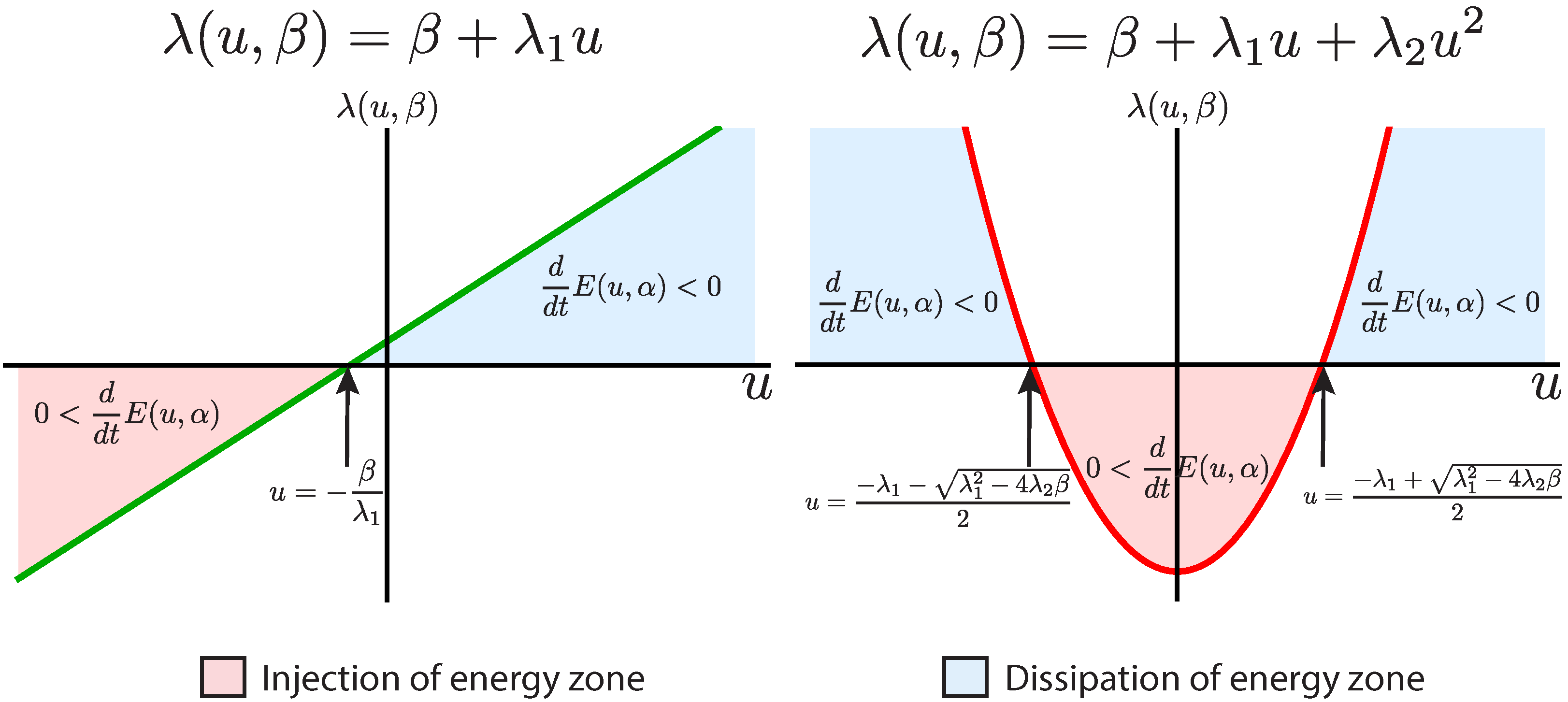
Figure 2. The left graphic shows in green a linear friction curve. The right graphic shows in red a quadratic friction curve with $0<{\lambda }_2$. The arrow indicates the points where the friction changes the sign in both cases. In pale red, we indicate the region where the system undergoes an injection of energy $0<\frac{d}{dt}E(u,\alpha )$ and in pale blue the region where the system undergoes a dissipation of energy $\frac{d}{dt}E(u,\alpha )<0$.

Figure 2. The left graphic shows in green a linear friction curve. The right graphic shows in red a quadratic friction curve with $0<{\lambda }_2$. The arrow indicates the points where the friction changes the sign in both cases. In pale red, we indicate the region where the system undergoes an injection of energy $0<\frac{d}{dt}E(u,\alpha )$ and in pale blue the region where the system undergoes a dissipation of energy $\frac{d}{dt}E(u,\alpha )<0$.

Since we know analytically the Jordan basis, we are able to calculate explicitly the cubic BT normal form using the methods developed in [2]; that is, to calculate for any model of the form of Equation (1), the explicit dependence of the unfolding parameters (α, β, ${\gamma }_2$) and the coefficients (${\gamma }_3$, ${\lambda }_1$, ${\lambda }_2$) on the parameters of the model. We find that the critical variables of the normal form can be chosen to be $(u,\dot{u})$, where u is the dimensionless membrane potential and $\dot{u}$ its time derivative (see Equation (1), Section 1.1, Supplementary Materials). The calculations, which are standard after the results in [2], are presented for the quadratic coefficient ${\gamma }_2$ (see Section 3, Supplementary Materials). Very surprisingly we found that the quadratic term of the force is proportional to the second derivative of the I-V curve, i.e.:

$${\gamma }_2\propto \frac{{\partial }^2{I}^{\infty }(u^{*};{\overrightarrow{\sigma }}_T,\overrightarrow{\eta })}{\partial u^2}$$

This relation is very important, since it shows that in order to have one or three fixed points (which is what is observed), then in the unfolding of the normal form, we have to impose an additional condition, namely that the second derivative of the I-V function with respect to u vanishes. This means that in the normal form, the calculated ${\gamma }_2$ will be very small (see Equation (18)). Therefore, we have to look for another scaling. The next scaling to consider is a quadratic friction, i.e., $\lambda (u,\beta )=\beta +{\lambda }_{1}u+{\lambda }_2{u}^2$. Since we are looking for a bounded dynamics, we must consider $0<{\lambda }_2$. As is shown in Figure 2 (right plot), for some values of u, i.e., $\frac{-{\lambda }_1-\sqrt{{\lambda }_1^2-4{\lambda }_2\beta }}{2}<u<\frac{-{\lambda }_1+\sqrt{{\lambda }_1^2-4{\lambda }_2\beta }}{2}$, there will be only the injection of energy, and it can be shown analytically that the system cannot have a stable fixed point in this region, no matter the form of the force. Therefore, all of the orbits will escape from this region, but the orbits will not go to infinity, because as soon as they reach the regions $\frac{-{\lambda }_1+\sqrt{{\lambda }_1^2-4{\lambda }_2\beta }}{2}<u$ or $u<\frac{-{\lambda }_1-\sqrt{{\lambda }_1^2-4{\lambda }_2\beta }}{2}$, the system will dissipate energy quadratically with the variable u and the dynamics will be bounded to a certain region of phase space. Then this scaling will present a bounded dynamics for sensible force functions. Moreover, it has been shown that the BT normal form with a quadratic friction and cubic force presents a rich set of global bifurcations, some of which are characteristic of single neuron dynamics [24]. The cubic BT normal form has the following form:

$$\ddot{u}=\alpha +{\gamma }_2{u}^2+{\gamma }_3{u}^3+\dot{u}\left(\beta +{\lambda }_{1}u+{\lambda }_2{u}^2\right)$$

(20)

This equation corresponds to the normal form of a particular BT bifurcation point of codimension three described by Equations (16)–(18). We expect that this normal form displays at least some of the fundamental aspects of single neuron dynamics, since we construct this critical point imposing constrains widely observed among neurons. However, it is not clear if this equation is able to reproduce the diversity in the observed dynamics of neurons. We show that it does in the next section.

4. Numerical Results and Comparison with the Morris–Lecar CB Model

Simulations of the cubic BT normal form show that the most typical global bifurcations mentioned in the literature for neuron models (i.e., saddle-node homoclinic bifurcation, the saddle-homoclinic bifurcation and the big homoclinic bifurcation) [4,7] are generically displayed by this equation.

Figure 3. In the phase space (top part of each figure) is symbolized with square nodes and saddle points and with a circle focus. The stable fixed points are purple, the unstable fixed points red and the saddle fixed points dark yellow. The linear stable manifold was colored blue and the linear unstable manifold colored yellow. The force $F(u,\alpha )$ is in blue and the friction $\lambda (u,\beta )$ in red. Repeller orbits are shown in black (middle figure). A sample of the dynamics is displayed at the bottom of each figure. The top, middle and bottom figures show a saddle-node homoclinic, big homoclinic and saddle homoclinic bifurcation, respectively, before, in and after the bifurcation. The arrows show the direction of the increasing of the unfolding parameters (α or β).

Figure 3. In the phase space (top part of each figure) is symbolized with square nodes and saddle points and with a circle focus. The stable fixed points are purple, the unstable fixed points red and the saddle fixed points dark yellow. The linear stable manifold was colored blue and the linear unstable manifold colored yellow. The force $F(u,\alpha )$ is in blue and the friction $\lambda (u,\beta )$ in red. Repeller orbits are shown in black (middle figure). A sample of the dynamics is displayed at the bottom of each figure. The top, middle and bottom figures show a saddle-node homoclinic, big homoclinic and saddle homoclinic bifurcation, respectively, before, in and after the bifurcation. The arrows show the direction of the increasing of the unfolding parameters (α or β).

The top plot in Figure 3 shows the saddle-node homoclinic scenario. Before the bifurcation, we have three fixed points: a stable node, a saddle and an unstable focus. As is shown numerically, if we follow the orbits in green, these two fixed points have a heteroclinic connection. The unstable focus is inside the heteroclinic connection. When we move the parameter α, these fixed points collide, and the heteroclinic connection becomes a limit cycle; this is the point where the saddle-node homoclinic bifurcation occurs. The unstable focus remains inside the limit cycle. This scenario is a distinctive bifurcation of Class I neurons.

The middle plot in Figure 3 shows the big homoclinic scenario. As in the last scenarios, there are three fixed points: a stable node, a saddle and an unstable focus. When we decrease the parameter β, the unstable manifold of the saddle fixed point returns, getting closer to the stable manifold. When the unstable manifold and the stable manifold connect by the same orbit, then the homoclinic orbit formed traps the other ends of the unstable and stable manifolds of the saddle, then the big homoclinic bifurcation occurs. This homoclinic connection becomes a limit cycle with the three fixed points inside. The limit cycle is separated of the unstable focus by a heteroclinic separatrix, as is shown in the third graphic of the figure in black. The separatrix connects the stable manifold of the saddle point with the unstable focus, forming a closed figure. This connection is generic (codimension zero) because it connects a stable manifold (dimension one) with the unstable manifold (dimension two) of the focus. This separatrix may suffer a saddle-homoclinic bifurcation, and we finally obtain a big limit cycle, a stable focus and a limit cycle separatrix in between. Then, moving the parameters, this limit cycle could collide and disappear. Together, these scenarios are distinctive for Class II neurons.

The bottom plot in Figure 3 shows the saddle homoclinic scenario. There are three fixed points: a stable node, a saddle and an unstable focus. When the parameter β increases, the unstable manifold of the saddle fixed point returns, getting closer to the stable manifold. When the unstable manifold and the stable manifold connect by the same orbit, the saddle homoclinic bifurcation occurs, and then, the homoclinic connection becomes a limit cycle. The unstable focus stays inside the limit cycle. The limit cycle (marked with 1 in the figure) and the stable node (marked with 2 in the figure) are separated by the stable manifold of the saddle point. This bistable behavior has been reported before in neural models [4,7]. In general, this bistable scenario is not necessarily the outcome of the saddle homoclinic bifurcation, but in neuron models, this is often the case. This scenario is also distinctive for Class II neurons.

We have compared these results with the dynamics observed in the Morris–Lecar model [13]. This CB model has been widely studied in computational neuroscience, and it is known that it displays much of the diversity observed in single neuron dynamics [4]. This is a minimal CB model, in the sense that it has the minimal number of variables for presenting oscillations (two variables). The nondimensional form of the Morris–Lecar model reads:

$$\begin{array}{ccc}\hfill \dot{u}& =& I-g_{1}n(u-u_1)-g_2{m}^{\infty }\left(u\right)(u-u_2)-g_3(u-u_3)\hfill \end{array}$$

(21)

$$\begin{array}{ccc}\hfill \dot{n}& =& \frac{n^{\infty }\left(u\right)-n}{\tau \left(u\right)}\hfill \end{array}$$

(22)

where $m^{\infty }\left(u\right)$, $n^{\infty }\left(u\right)$ and $\tau \left(u\right)$ are hyperbolic functions (see Equations (34)–(36), Section 4, Supplementary Materials). We transformed this model to a second order differential equation form (for details, see Section 4.2, Supplementary Materials) that reads:

$$\ddot{u}=\frac{I-I^{\infty }\left(u\right)}{\tau \left(u\right)}-\dot{u}\left(\frac{I-I^{\infty }\left(u\right)}{u-u_1}+\frac{\partial I^{\infty }\left(u\right)}{\partial u}+\frac{1-G\left(u\right)}{\tau \left(u\right)}\right)+\frac{{\dot{u}}^2}{u-u_1}$$

(23)

where $G\left(u\right)$ is the gating function of the slow gating variable n (Equation (55), Section 4.2, Supplementary Materials). Surprisingly, the transformed equation has almost the same form of the cubic BT normal form: a cubic-like force and a quadratic-like friction (see Figure 4), but also a term proportional to ${\dot{u}}^2$. In Figure 4, we showed the simultaneous simulation of the full Morris–Lecar model, the Morris–Lecar model without the term proportional to ${\dot{u}}^2$ and a reduced version, where we also removed the $\frac{I-f\left(u\right)}{u-u_1}\dot{u}$ term (to test the effect of the singularity in the friction term at $u=u_1$). The force term in all of the equations is the same, and interestingly, it is proportional to the injected current minus the I-V curve, which will vanish when it is evaluated at a fixed point. Figure 4 shows the clear cubic-like shape of the force and also the quadratic shape, in the relevant region for the dynamics, of the friction. The quadratic shape of the friction is present in both cases, with and without the $-\frac{I-f\left(u\right)}{u-u_1}\dot{u}$ term, with slight differences between the two friction curves. We found the same global bifurcation scenarios as in the cubic BT normal form (i.e., saddle-node homoclinic, big homoclinic and saddle homoclinic bifurcation) in the three versions of the model. The dynamics does not change qualitatively, but quantitatively, with differences in the specific value of I when a global bifurcation occurs, the shape and period of the limit cycles and the shape of the separatrices. However, this is expected, since it is known that global bifurcations are dependent on nonlinearities.

These last results are remarkable by themselves: we found that the Morris–Lecar model is in practice equivalent to the cubic BT normal form for realistic values of parameters. However, most importantly, these simulations consistently support our theoretical results showing that the dynamics observed in the original CB models are explained by the cubic BT normal form.

The parameters used for simulations in Figure 3 and Figure 4 can be found in Section 5 of the Supplementary Materials.

Figure 4. Simultaneously simulated full Morris–Lecar model (green), Morris–Lecar without the term proportional to ${\dot{u}}^2$ (yellow) and the reduced Morris–Lecar (purple) for three different values of parameters. The force term ($\frac{I-f\left(u\right)}{\tau \left(u\right)}$) is the same for the three equations, and we plot it in the phase plane in blue. For the full Morris–Lecar model and Morris–Lecar without the term in ${\dot{u}}^2$, the friction curve is displayed in red, for the reduced model in magenta. The top, middle and bottom figures show a saddle-node homoclinic, big homoclinic and saddle homoclinic bifurcation, respectively, before, in and after the bifurcation. The arrows show the direction of increasing of I. The same shapes and color codes in Figure 3 are used.

Figure 4. Simultaneously simulated full Morris–Lecar model (green), Morris–Lecar without the term proportional to ${\dot{u}}^2$ (yellow) and the reduced Morris–Lecar (purple) for three different values of parameters. The force term ($\frac{I-f\left(u\right)}{\tau \left(u\right)}$) is the same for the three equations, and we plot it in the phase plane in blue. For the full Morris–Lecar model and Morris–Lecar without the term in ${\dot{u}}^2$, the friction curve is displayed in red, for the reduced model in magenta. The top, middle and bottom figures show a saddle-node homoclinic, big homoclinic and saddle homoclinic bifurcation, respectively, before, in and after the bifurcation. The arrows show the direction of increasing of I. The same shapes and color codes in Figure 3 are used.

5. Conclusions

Using as a starting point a generic CB model, we looked for a critical point that encloses the diversity of local bifurcations observed in single neuron dynamics. In order to do that, we first constrained the general model to be in a critical point that possesses both local saddle-node and Andronov–Hopf bifurcations in its neighborhood. By using theoretical considerations, we concluded that this critical point is the BT bifurcation. In order to include the experimentally-observed curvatures of the I-V curve within the neighborhood of the critical point, we further constrained the model to be in the transition between one to three fixed points. This led us naturally to conclude that the BT normal form at this particular point must be cubic. Then, the dynamics of any CB model that is in some neighborhood of this particular BT bifurcation should be qualitatively captured by this equation. Our simulations showed that, in fact, it robustly displays much of the features observed in single neuron dynamics. Furthermore, we numerically found that the Morris–Lecar model, one of the most widely-used CB models, is in practice equivalent to the cubic BT normal form for realistic parameters values. These results might be explained by the fact that we construct the critical point imposing general features that are robustly observed among neurons. Additionally, by so doing, we obtained a critical point that correspond to a realistic parameter range for CB models. Hence, moderate displacements from this point in the space of parameters by different CB models, which represent different types of neurons, will still lay in the region where this normal form is qualitatively valid. This is consistent with the fact that this model cannot describe more unusual scenarios when, for example, a third, very long time scale conductance is introduced, and CB models display a dynamics, named bursting. This type of dynamics is generically well described by models of at least three equations [25]. We believe that it is necessary to impose a further constraint on the critical point to arrive at a three-variable normal form that successfully reproduces this type of behavior. Recently, we gave some steps toward that direction [1].

In light of our theoretical findings and numerical results, we propose the cubic BT normal form as a minimal model for single neuron dynamics that naturally arises from CB models.

References

1. Pereira, U. Toward a Universal Description for Single Neuron Dynamics. Master’s Thesis, Universidad de Chile, Santiago, Chile, 2013. [Google Scholar]
2. Elphick, C.; Tirapegui, E.; Brachet, M.E.; Coullet, P.; Iooss, G. A simple global characterization for normal forms of singular vector fields. Physica D 1987, 29, 95–127. [Google Scholar] [CrossRef]
3. Haragus, M.; Iooss, G. Local Bifurcations, Center Manifolds, and Normal Forms in Infinite-Dimensional Dynamical Systems, 1st ed.; Springer: New York, NY, USA, 2011. [Google Scholar]
4. Ermentrout, G.B.; Terman, D.H. Mathematical Foundations of Neuroscience, 1st ed.; Springer: New York, NY, USA, 2010. [Google Scholar]
5. Carnevale, N.T.; Hines, M.L. The NEURON Book; Cambridge University Press: Cambridge, UK, 2006. [Google Scholar]
6. Dayan, P.; Abbott, L.F. Theoretical Neuroscience; The MIT Press: Cambridge, MA, USA, 2001; Volume 806. [Google Scholar]
7. Izhikevich, E.M. Dynamical Systems in Neuroscience: The Geometry of Excitability and Bursting; The MIT Press: Cambridge, MA, USA, 2010. [Google Scholar]
8. Ranjan, R.; Khazen, G.; Gambazzi, L.; Ramaswamy, S.; Hill, S.L.; Schurmann, F.; Markram, H. Channelpedia: An integrative and interactive database for ion channels. Front. Neuroinform. 2011, 5. [Google Scholar] [CrossRef] [PubMed]
9. Peterson, B.E.; Healy, M.D.; Nadkarni, P.M.; Miller, P.L.; Shepherd, G.M. ModelDB: An environment for running and storing computational models and their results applied to neuroscience. J. Am. Med. Inform. Assoc. 1996, 3, 389–398. [Google Scholar] [CrossRef] [PubMed]
10. Hodgkin, A. The local electric changes associated with repetitive action in a non-medullated axon. J. Physiol. 1948, 107, 165–181. [Google Scholar] [CrossRef] [PubMed]
11. Rinzel, J.; Ermentrout, G.B. Analysis of neural excitability and oscillations. Method. Neuron. Model. 1998, 2, 251–292. [Google Scholar]
12. FitzHugh, R. Mathematical models of threshold phenomena in the nerve membrane. Bull. Math. Biophys. 1955, 17, 257–278. [Google Scholar] [CrossRef]
13. Morris, C.; Lecar, H. Voltage oscillations in the barnacle giant muscle fiber. Biophys. J. 1981, 35. [Google Scholar] [CrossRef]
14. Kepler, T.B.; Abbott, L.; Marder, E. Reduction of conductance-based neuron models. Biol. Cybern. 1992, 66, 381–387. [Google Scholar] [CrossRef] [PubMed]
15. Hodgkin, A.L.; Huxley, A.F. A quantitative description of membrane current and its application to conduction and excitation in nerve. J. Physiol. 1952, 117, 500–544. [Google Scholar] [CrossRef] [PubMed]
16. Johnston, D.; Wu, S.M.S.; Gray, R. Foundations of Cellular Neurophysiology; The MIT press: Cambridge, MA, USA, 1995. [Google Scholar]
17. Pereira, U.; Tirapegui, E. Una Ecuación Universal Para la Dinámica Neuronal. In Processdings of the XVII Conference on Nonequilibrium Statistical Mechanics and Nonlinear Physics, Santiago, Chile, 3–7 December 2012.
18. Pereira, U.; Tirapegui, E. Una Ecuación Universal Para la Dinámica Neuronal. In Proceedings of the XVIII Simposio Chileno de Física, La Serena, Chile, 21–23 November 2012.
19. Hille, B. Ion Channels of Excitable Membranes; Sinauer: Sunderland, MA, USA, 2001; Volume 507. [Google Scholar]
20. Sherman, J.; Morrison, W.J. Adjustment of an Inverse Matrix Corresponding to a Change in One Element of a Given Matrix. Ann. Math. Statist. 1950, 21, 124–127. [Google Scholar] [CrossRef]
21. Ding, J.; Zhou, A. Eigenvalues of rank-one updated matrices with some applications. Appl. Math. Lett. 2007, 20, 1223–1226. [Google Scholar] [CrossRef]
22. Kuznetsov, Y.A. Elements of Applied Bifurcation Theory, 2nd ed.; Springer: New York, NY, USA, 2004. [Google Scholar]
23. Guckenheimer, J.; Holmes, P. Nonlinear Oscillations, Dynamical Systems, and Bifurcations of Vector Fields, 7th ed.; Springer: New York, NY, USA, 2002. [Google Scholar]
24. Kuznetsov, Y.A. Practical computation of normal forms on center manifolds at degenerate Bogdanov–Takens bifurcations. Int. J. Bifurc. Chaos 2005, 15, 3535–3546. [Google Scholar] [CrossRef]
25. Coombes, S.; Bressloff, P.C. Bursting: The Genesis of Rhythm in the Nervous System, 1st ed.; World Scientific: Singapore, Singapore, 2005. [Google Scholar]
26. Kirst, C.; Ammer, J.; Felmy, F.; Herz, A.; Stemmler, M. Fundamental Structure and Modulation of Neuronal Excitability: Synaptic Control of Coding, Resonance, and Network Synchronization. bioRxiv 2015, 022475. [Google Scholar]