Multidimensional Scaling Visualization Using Parametric Similarity Indices

Abstract

In this paper, we apply multidimensional scaling (MDS) and parametric similarity indices (PSI) in the analysis of complex systems (CS). Each CS is viewed as a dynamical system, exhibiting an output time-series to be interpreted as a manifestation of its behavior. We start by adopting a sliding window to sample the original data into several consecutive time periods. Second, we define a given PSI for tracking pieces of data. We then compare the windows for different values of the parameter, and we generate the corresponding MDS maps of ‘points’. Third, we use Procrustes analysis to linearly transform the MDS charts for maximum superposition and to build a global MDS map of “shapes”. This final plot captures the time evolution of the phenomena and is sensitive to the PSI adopted. The generalized correlation, the Minkowski distance and four entropy-based indices are tested. The proposed approach is applied to the Dow Jones Industrial Average stock market index and the Europe Brent Spot Price FOB time-series.

1. Introduction

Complex systems (CS) are frequent in many natural (e.g., geophysics, cosmology, ecology, biology, genetics) and man-made (e.g., economy, computer science, chemical and physical apparatus) systems [1–10]. They are often constituted by multiple interacting entities that contribute to a collective behavior revealing surprising dynamical phenomena. CS modeling can adopt sophisticated mathematical tools, but often, we verify that those methods are still far from capturing the overall richness of the system evolution. Therefore, a fruitful interplay is possible by experimenting in a given case with mathematical tools that are usual in distinct areas [11].

Multidimensional scaling (MDS) is a computer method for visualizing and comparing data that have been applied in many distinct areas [12–15]. Polzella and Reid [16] used MDS in the study of pilot performance data obtained during simulated combat. Costa et al. [17] considered MDS to analyze DNA code in the perspective of identifying structural patterns in the nuclear and mitochondrial genomes. Machado et al. [18] adopted MDS to study fifteen stock markets and to unveil time-varying correlations between them. Oñate and Pou [19] analyzed the temperature time-series from eleven meteorological stations over the Iberian Peninsula. Trends were identified by means of Mann–Kendall tests, while MDS was employed to build automatic grouping. More recently, Stephenson and Doblas-Reyes [20] used MDS as an exploratory tool for describing ensembles of forecasts. Lopes and Machado [11] studied global temperature time-series, showing that MDS is able to provide an intuitive and useful visual representation of the complex relationships present in the data.

In this paper, we combine MDS tools and parametric similarity indices (PSI) in the analysis of CS. Each phenomenon is viewed as a dynamical system whose output is a time-series. The time-series are interpreted as manifestations of the system behavior. The novel methodology is structured as follows. First, we adopt a sliding time-window to convert the original data into smaller parts that reflect evolution in time. Second, for a given PSI, we compare the time-windows for different values of the parameter, and we generate the corresponding MDS maps of “points”. Third, we transform the individual MDS charts for obtaining the maximum object superposition. The construction of the global MDS map unveils the characteristics of the CS.

Our approach represents a generalization of MDS classical schemes. In fact, standard MDS representations capture the system dynamics by means of a single similarity index. Such an index depends of the researcher’s choice, and therefore, we can define distinct criteria. The MDS interpretation is based on the emerging clusters and distances between “objects” (“points”) in the map, rather than on their absolute coordinates or the geometrical form of the locus. We propose subdividing each time-series into several smaller slices, to capture time dynamics, and to adopt PSI in each MDS map, providing distinct comparisons for the same windows. The interpretation of the MDS map is now based on “objects” consisting of “shapes” (a collection of points) instead of “points”, capturing the time evolution of the phenomena and being sensitive to the parametric index adopted.

Loosely speaking, with the standard MDS methods, we are viewing “objects” under a monochrome beam of light, while with the PSI approach, we vary the light wavelength, leading to a more colorful and detailed characterization of the “objects”.

The generalized correlation, Minkowski distance and entropy are tested as candidates for the parameter-dependent comparison indices. The proposed approach is applied to the Dow Jones Industrial Average stock market index (DJ) and Europe Brent Spot Prices FOB (BR) time-series.

Bearing these ideas in mind, this paper is organized as follows. Section 2 introduces the main mathematical tools used for processing the data. Section 3 analyses real data by means of several PSI and MDS. Finally, Section 4 outlines the main conclusions.

2. Mathematical Tools

This section formulates the main mathematical tools adopted for data numerical analysis. Section 2.1 presents the PSI, namely the generalized correlation, the Minkowski distance and the entropy-based indices. Section 2.2 addresses the MDS technique.

2.1. Parametric Similarity Indices

2.1.1. Generalized Correlation

Given two random variables X and Y, its generalized correlation coefficient is expressed by [21]:

$${\rho }_q=\frac{E\left[g_q(X_i-X_j)g_q(Y_i-Y_j)\right]}{\sqrt{E\left[g_{{}_q}^2(X_i-X_j)\right]E\left[g_{{}_q}^2(Y_i-Y_j)\right]}}$$

(1)

where E(·) denotes the expectation operator and (X_i, Y_i) and (X_j, Y_j) are independent bivariate vectors with i ≠ j, (i, j) = 1, 2, …, n. The function g_q(z) in Equation (1) is given by:

$$g_q(z)=\mathrm{sign}(z)|z{|}^q,q\in [0,1]$$

(2)

The generalized correlation is always in the interval ρ_q ∈ [−1, 1] with lower and upper values corresponding to the Kendall, ρ_K, and Pearson, ρ_P, correlation coefficients, respectively:

$${\rho }_K=\frac{E\left[\mathrm{sign}(X_i-X_j)\mathrm{sign}(Y_i-Y_j)\right]}{\sqrt{E\left[{\mathrm{sign}}^2(X_i-X_j)\right]E\left[{\mathrm{sign}}^2(Y_i-Y_j)\right]}}$$

(3)

$${\rho }_P=\frac{E\left[(X_i-X_j)(Y_i-Y_j)\right]}{\sqrt{E\left[{(X_i-X_j)}^2\right]E\left[{(Y_i-Y_j)}^2\right]}}$$

(4)

Expression (1) is a general parametric statistics with an extra degree of freedom, q, that can be tuned by the user according to the problem under analysis.

The generalized correlation coefficient of a sample, ${\widehat{\rho }}_q$, can be estimated by means of:

$${\widehat{\rho }}_q=\frac{U_q{{}_{,}}_{XY}}{\sqrt{U_q{{}_{,}}_{XX}{U}_q{{}_{,}}_{YY}}}$$

(5)

where,

$$U_q{{}_{,}}_{XY}=\frac{2}{n(n-1)}{\displaystyle \sum _{i<j}^n{g}_q(X_i-X_j)g_q(Y_i-Y_j)}$$

(6)

$$U_q{{}_{,}}_{XX}=\frac{2}{n(n-1)}{\displaystyle \sum _{i<j}^n{g}_{{}_q}^2(X_i-X_j)}$$

(7)

$$U_q{{}_{,}}_{YY}=\frac{2}{n(n-1)}{\displaystyle \sum _{i<j}^n{g}_{{}_q}^2(Y_i-Y_j)}$$

(8)

2.1.2. Minkowski Distance

The Minkowski distance is a metric on the Euclidean space that generalizes other distances [22].

Given two points X = (x₁, x₂, …,x_n) and Y = (y₁, y₂, …, y_n) in ${\mathrm{ℝ}}^n$, the q-order Minkowski distance is expressed by:

$$d_q={\left({\displaystyle \sum _{i=1}^n|x_i-y_i{|}^q}\right)}^{1/q},q\in \mathrm{ℝ}$$

(9)

For q = 1, Expression (9) yields the Manhattan distance; for q = 2, we have the Euclidean distance; and for q → ∞, we obtain the Chebyshev distance.

2.1.3. Entropy

Entropy has been used not only in the context of CS, but also in many other scientific areas [23–25]. In information theory, entropy was introduced by Shannon for studying the amount of information contained in a message. Shannon entropy satisfies the so-called Khinchin axioms [26] and is given by:

$$S={\displaystyle \sum _i(-\ln p_i)}{p}_i$$

(10)

Entropy represents the expected value of the information content, I(p_i) = − ln p_i, of an event with probability of occurrence p_i, where ${\displaystyle \sum _i{p}_i=1}$.

Rényi and Tsallis entropies are generalizations of Shannon’s entropy and are given by, respectively:

$$S_q^{(R)}=\frac{1}{1-q}\ln \left({\displaystyle \sum _i{p}_i^q}\right),q\in {\mathrm{ℝ}}^{+}$$

(11)

$$S_q^{(T)}=\frac{1}{q-1}\left(1-{\displaystyle \sum _i{p}_i^q}\right),q\in \mathrm{ℝ}$$

(12)

Inspired by the concepts of fractional calculus (FC), Ubriaco [27] proposed the following expression:

$$S_q^{(U)}={\displaystyle \sum _i{(-\ln p_i)}^q{p}_i}$$

(13)

that has the same properties as the Shannon entropy, except additivity. Rényie, Tsallis and Ubriaco entropies reduce to Shannon’s expression when q → 1.

FC denotes the branch of calculus that extends the concepts of integrals and derivatives to non-integer and complex orders. During the last few decades, FC was found to play a fundamental role in modeling many important physical phenomena and emerged as an important tool in the area of dynamical systems [28–30].

Recently, also inspired by FC, the concepts of information content and entropy of order $q\in \mathrm{ℝ}$, $I_q^{(G)}$ and $S_q^{(G)}$, were proposed [31,32]. These generalizations of the classical definitions are given by:

$$I_q^{(G)}(p_i)=D^{q}I(p_i)=-\frac{p_i{}^{-q}}{\mathrm{\Gamma }(q+1)}[\ln p_i+\psi (1)-\psi (1-q)]$$

(14)

$$S_q^{(G)}={\displaystyle \sum _i\left\{-\frac{p_i{}^{-q}}{\mathrm{\Gamma }(q+1)}[\ln p_i+\psi (1)-\psi (1-q)]\right\}}{p}_i$$

(15)

where D^q (·) is the fractional derivative of order q and Γ (·) and ψ (·) represent the gamma and digamma functions, respectively.

The generalized entropy (15) does not obey some of the Khinchin axioms, except for q = 0 [31]. In this case, it leads to the classical Shannon entropy (10).

2.2. Multidimensional Scaling

MDS is a technique for visualizing information that explores similarities in data [33–37]. The main idea is to detect underlying dimensions that allow the researcher to observe similarities between the items under analysis. The MDS algorithm requires the definition of a similarity index and the construction of a h × h matrix M of item to item similarities, where h is the total number of items. In classical MDS, matrix M is symmetric, and its main diagonal is composed of “1”. MDS assigns a coordinate point to each item in a multi-dimensional space and arranges the set of h coordinates in order to reproduce the observed similarities. Often, instead of similarities, there are considered dissimilarities, or distances, between the items. For low dimensional spaces (e.g., m = 2 or m = 3) the resulting “points” can be displayed in a “map”. As mentioned, by rearranging the item positions in the space, MDS tries to arrive at a configuration that best approximates the observed similarities. For this purpose, MDS uses a function minimization algorithm that evaluates different configurations with the goal of maximizing the goodness-of-fit. A common measure to evaluate how well a particular configuration reproduces the observed distance matrix is the raw stress, $\mathcal{S}$, in general defined as:

$$\mathcal{S}={[d_{ij}-f({\delta }_{ij})]}^2$$

(16)

where d_ij stands for the reproduced distances between items i and j, (i, j) = {0, 1, 2, …, h − 1}, δ_ij represents the observed distances and f(·) indicates some type of transformation. The smaller the value of $\mathcal{S}$, the better is the fit between d_ij and δ_ij.

We can rotate or translate the MDS map, since the distances between “points” remain identical.

The quality of the MDS approach can be evaluated by means of the stress and Shepard plots. The stress plot represents $\mathcal{S}$ versus the number of dimensions m of the MDS map. We get a monotonic decreasing chart, and we choose m as a compromise between reducing $\mathcal{S}$ and having a low dimension for the MDS map. The Shepard diagram compares the d_ij distances, for a particular value m, versus the δ_ij distances. Therefore, a narrow scatter around the 45-degree line indicates a good fit between d_ij and δ_ij.

3. MDS Analysis and Visualization of Complex Systems

In this section, we apply PSI and MDS tools in the analysis of real-world time-series. In Section 3.1, we use a simple example to introduce the approach. In Sections 3.2, 3.3 and 3.4, we process data from two CS by means of the generalized correlation index, the Minkowski distance and entropy, respectively. We use DJ and BR time-series at a daily time horizon [38,39] to characterize the CS dynamics. The data are available at the Yahoo Finance ( https://finance.yahoo.com/) and the U.S. Energy Information Administration ( http://www.eia.gov/) websites. The time period of analysis is from 20 May 1987, up to 5 January 2015. Some missing values are estimated by means of a linear interpolation algorithm, applied between neighbor values, so that all weeks have five values.

3.1. Illustrative Example

Given a time-series representative of a CS over the period T, $\tilde{x}(t)$, 0 ≤ t < T, we divided the data into h intervals, denoted by x_k(t), kT/h ≤ t < (k + 1)T/h, k = {0, 1, 2, …, h − 1}. For a PSI, we calculate p similarity matrices, M_q, h × h dimensional, where q ∈ {q₁, q₂,…, q_p}. Matrices M_q feed the MDS algorithm, which generates p intermediate maps of “points” (i.e., one map per value q). The charts are then processed by means of Procrustes analysis in order to obtain a single global plot of “shapes” where the “points” of the original maps are optimally “superimposed”.

Procrustes analysis performs linear transformations, namely translation, reflection, orthogonal rotation and scaling, with the objective of minimizing a measure of the difference between the “points” in the original maps. The algorithm: (i) chooses a reference MDS map (by selecting one of the available instances); (ii) superimposes all other MDS instances into the current reference; (iii) computes the mean form of the current set of superimposed maps; (iv) compares the distance between the mean and the reference instances to a given threshold value and, if above, sets the reference to the mean form and continues to Step (ii).

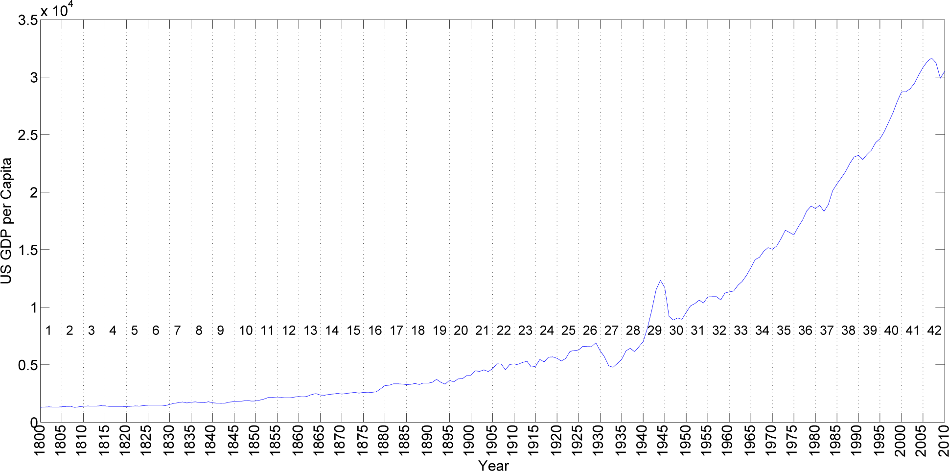
For illustrating our approach, we start by using a time-series consisting of the U.S. GDP per capita, for the period from year 1800 up to 2010, with units of 1990 GK dollars per capita. This time-series has the advantage of being simple and smooth over time, but rich enough to be used as an illustrative example. The data are from the Maddison Project [40].

Figure 1 shows the GDP time-series divided into h = 42 non-overlapping intervals of five years each. We adopt the Minkowski distance (9) with p = 22 parameter values and q varying uniformly in the interval q ∈ [0.12, 1.20]. We then calculate the matrices $M_q=\left[d_q^{ij}\right]$, (i, j) = 0, …, 41, that constitute the input for the MDS algorithm.

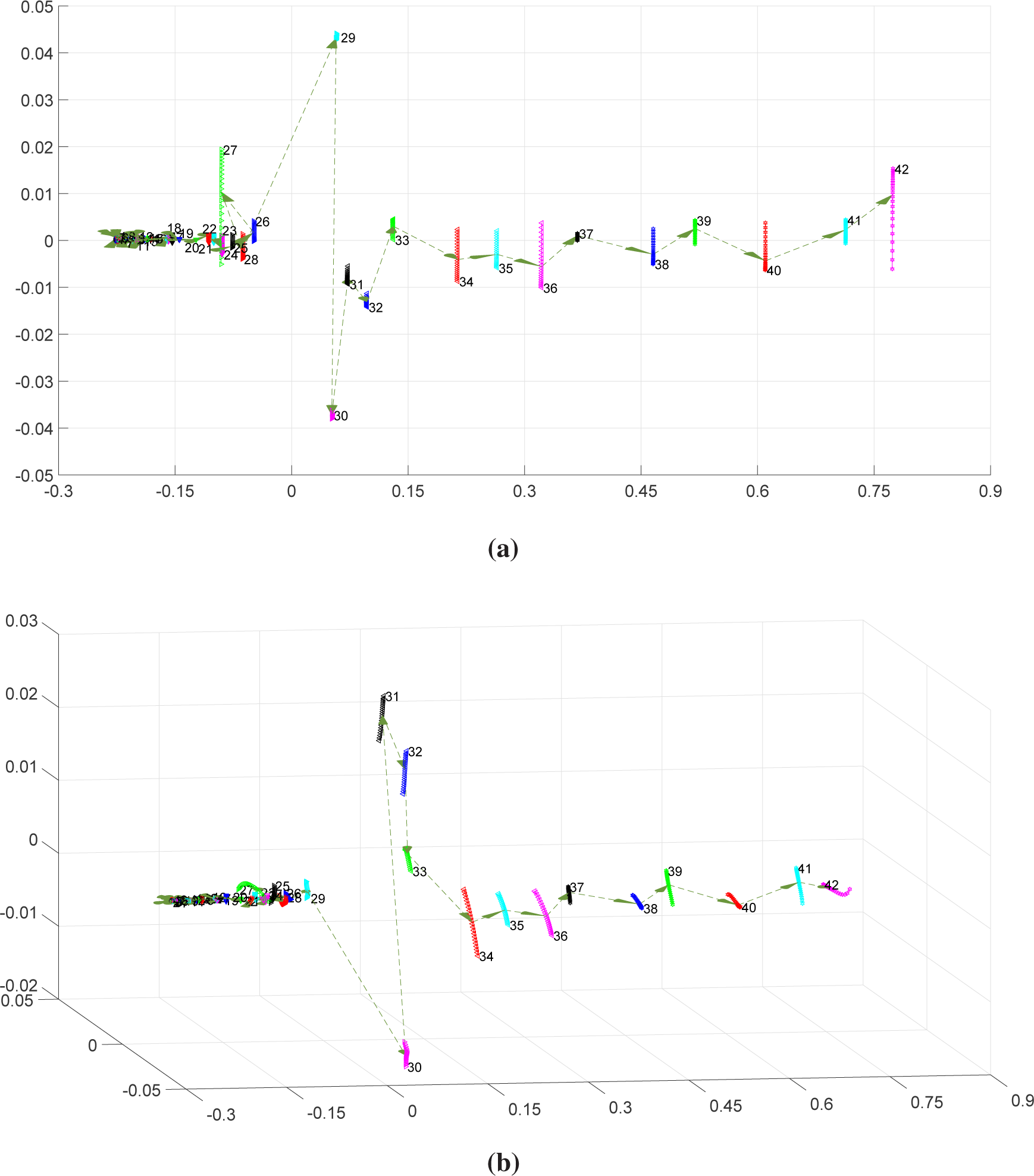
Figure 2 depicts the two- and three-dimensional global MDS maps that result from the Procrustes analysis. In these charts, we get a continuous set of p points for each time-window, meaning that we have maps of “shapes”, instead of merely “points”. We verify that the “shapes” have a one-dimensional nature and that their length varies along time. For example, “shapes” of windows {27, 31, 32, 34, 36, 42} exhibit a larger length, meaning that they are more sensitive to the variation of q.

Superimposed to the global maps, we represent the time behavior of the CS by means of a set of oriented arrows that connect the window “shapes” and indicate the flow of time. We verify longer “jumps” between certain time-windows, namely {29–30, 30–31, 31–32, 32–33, 33–34}, which means that they have different characteristics from the rest.

The following list emphasizes the relationships between the GDP time-series and the MDS global maps:

• During the time period 1800–1930, the GDP had a moderate growth with small oscillations over time. In the MDS maps, we observe small “shapes”, representing Windows 1 up to 26, appearing in sequence and close to each other;
• In the time period 1930–1935, corresponding to the worst years of the Great Depression, the GDP had a strong oscillation, increasing (with small fluctuation) during the subsequent five-year period, 1935–1940. Such behavior is observed in the MDS maps as two moderate length “jumps” from Window 26 towards Window 27 and then towards Window 28;
• Periods 1940–1945, 1945–1950 and 1950–1955 had contrasting behavior, characterized by growth and recession, mostly determined by World War II. In the MDS maps, we observe large “jumps” across Windows 29 up to 31;
• For the time period 1955–1960, GDP growth became slower and then recovered during the period 1960–1965. This corresponds to large “jumps” across Windows 31, 32 and 33 in the MDS;
• From year 1960 onward, we observe a GDP moderate growth trend, with oscillations over time. This behavior translates into moderate, and similar, length “jumps” between shapes in the MDS maps.

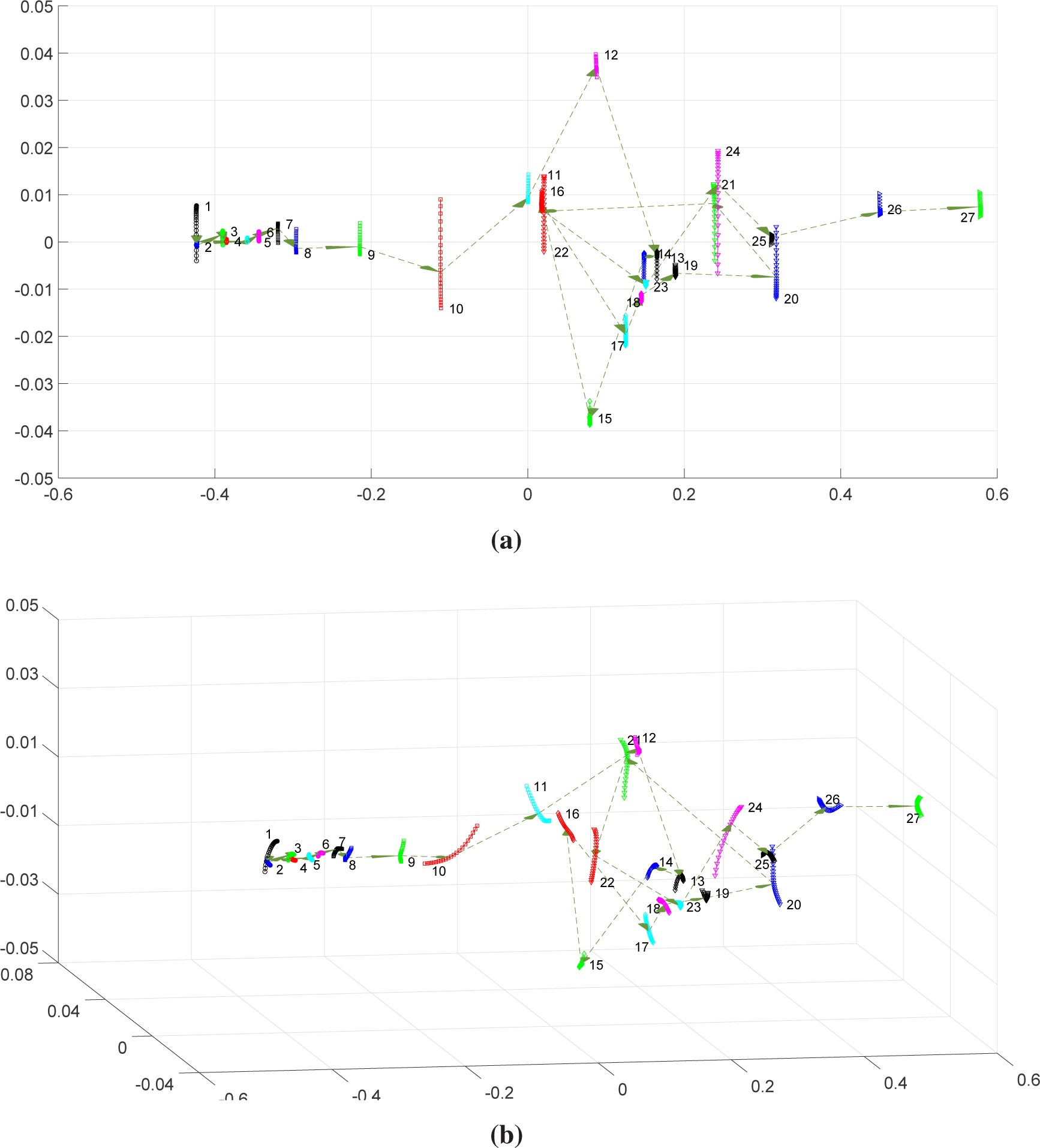
3.2. MDS Based on the Generalized Correlation Index

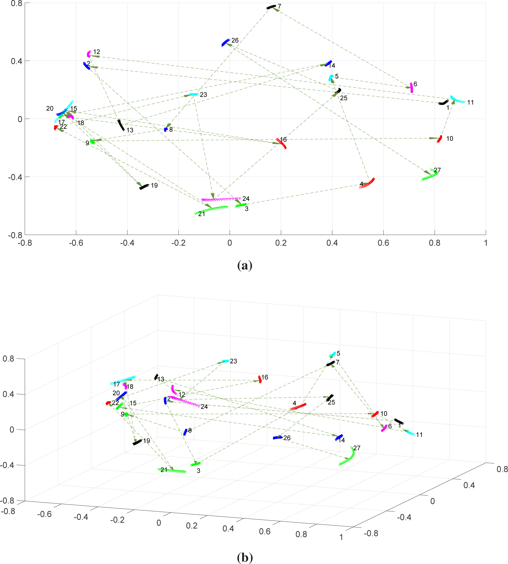
We start by dividing the total DJ series into h = 27 non-overlapping intervals of approximately a one-year time-length each. This value of h mitigates the problems related to the non-stationarity of the data and establishes a good compromise between time discrimination and solid histogram representation. We then adopt p = 22 distinct parameter values, uniformly distributed in the interval q ∈ [0, 1], and we calculate the corresponding matrices $M_q=\left[{\rho }_q^{ij}\right]$, (i, j) = 0, …, 26, where ${\rho }_q^{ij}$ represents the generalized correlation between x_i(t) and x_j(t).

Figure 3 shows the two- and three-dimensional MDS maps obtained after Procrustes analysis. We can see that the generalized correlation index leads successfully to maps of one-dimensional “shapes”. Windows {1, 5, 14, 18, 19, 21, 22, 23, 25} are more sensitive to the variation of q, since they are larger than the others. Furthermore, we observe the emergence of two main clusters of “shapes”: $\mathcal{A}=\left\{1,13,14,15,17,18,21,24\right\}$ and $\mathcal{B}=\left\{2,3,4,5,6,7,8,9,10,11,12,16,19,20,22,23,25,26,27\right\}$.

We verify longer “jumps” between certain time-windows, namely {1–2, 3–4, 15–16, 20–21, 21–22}, which means that they have distinctive characteristics. Nevertheless, we can see that ρ_q reveals difficulties with time flow discretization, since we obtain a large number of chaotic “jumps” between “shapes”.

The length of the “shapes” seems to be closely related to the annual volatility of the DJ stock market. In fact, windows exhibiting a larger length correspond to higher volatility time periods of the DJ. On the other hand, longer “jumps” seem to be related to periods of stock market crashes and bear markets, namely the “Black Monday of 1987” (Windows 1–2), the “Friday the 13th 1989 mini-crash” (3–4) the “Stock market downturn of 2002” (Windows 15–16) and the “United States bear market of 2007–2009” (Windows 20–21 and 21–22).

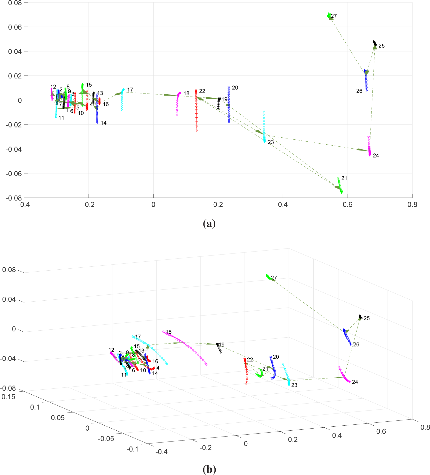
Identically to the DJ data, we process the BR time-series. Figure 4 shows the two- and three-dimensional MDS maps of “shapes” and the time behavior of the CS obtained after Procrustes analysis. In this case, two main clusters of “shapes” emerge: $\mathcal{A}=\left\{1,4,5,6,7,10,11,14,16,25,26,27\right\}$ and $\mathcal{B}=\left\{2,3,8,9,12,13,15,17,18,19,20,21,22,23,24\right\}$. Larger length “shapes” correspond to Windows {1, 2, 9, 11, 13, 14. 27}, while longer “jumps” correspond to Periods {4–5, 12–13, 17–18, 20–21, 21–22, 24–25, 26–27}. As for the DJ, ρ_q leads to a poor time discrimination between the data.

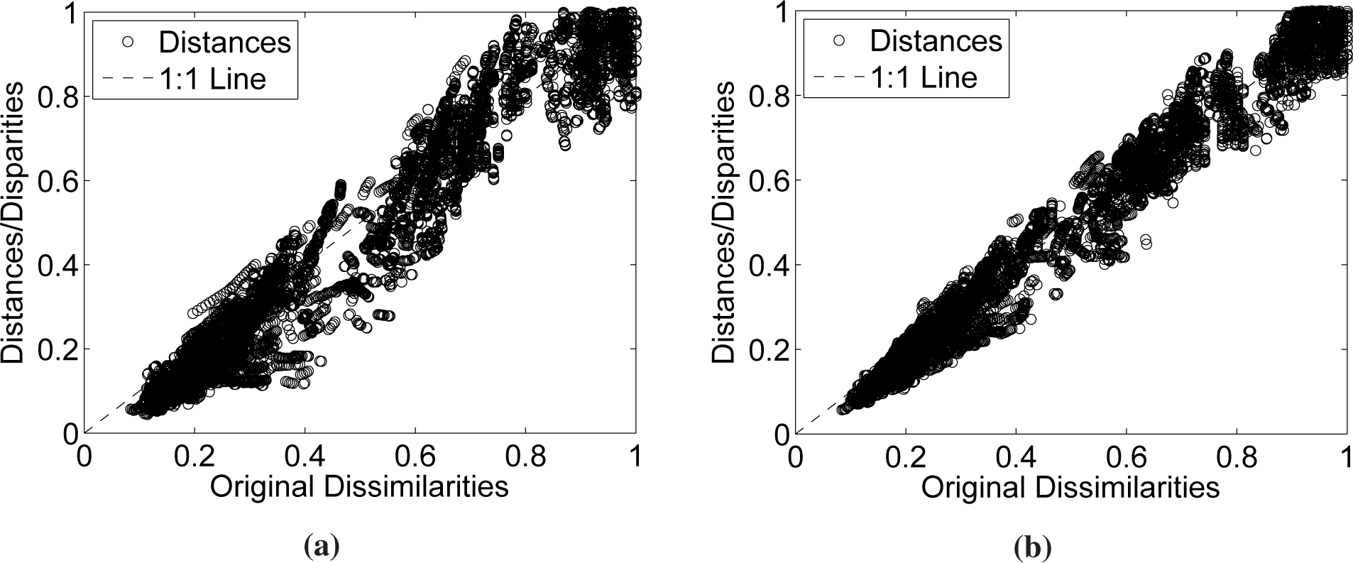
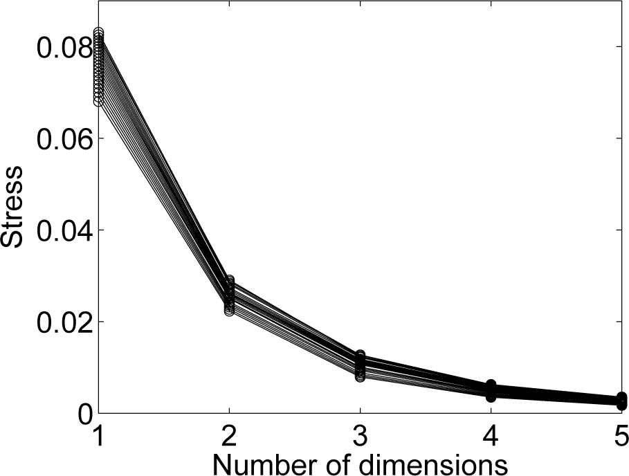
To assess the quality of the p intermediate MDS maps that are used to construct the global map of “shapes”, we plot the Shepard and the stress diagrams. We illustrate the results obtained for the DJ time-series and ρ_q. For the BR data, and for all PSI, the results are similar. Figure 5 represents the p Shepard diagrams superimposed in a single chart. We can observe a scatter of points distributed around the 45-degree line, which means a good fit of the observed distances to the dissimilarities. As expected, for m = 3, we get slightly better results than for m = 2. Figure 6 depicts the superposition of the stress diagrams, revealing that, for the p intermediate MDS maps, a three-dimensional space describes the data well.

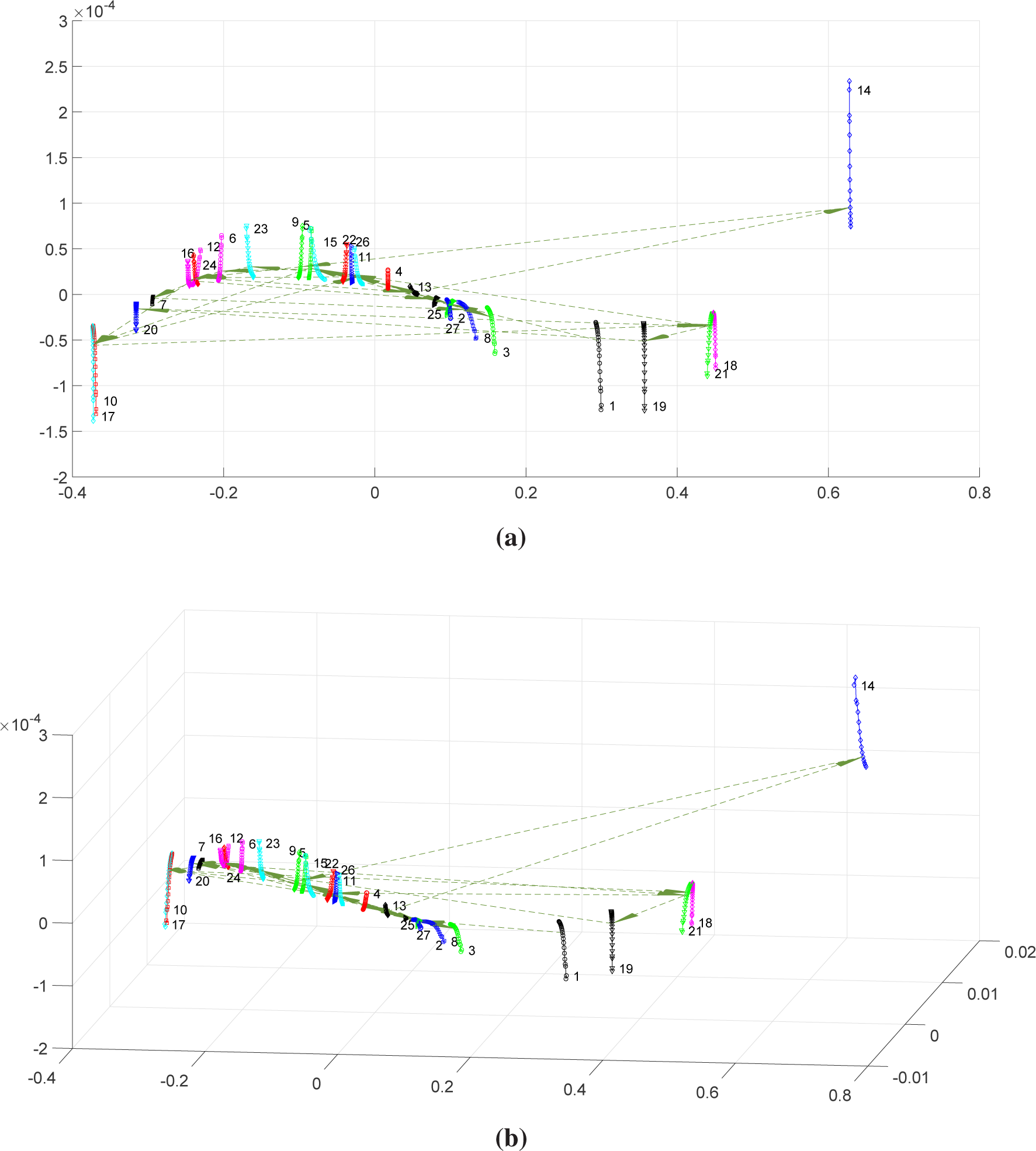
3.3. MDS Based on Minkowski Distance

In this subsection, we embed the Minkowski distance (9) into the MDS. The parameter q varies uniformly in the interval q ∈ [0.12, 1.20]. The remaining parameters stay unchanged with respect to Section 3.2. We calculate the matrices $M_q=\left[d_q^{ij}\right]$, and we use them as the input for the MDS algorithm.

Figures 7 and 8 depict the two- and three-dimensional MDS maps for the DJ and BR time-series, respectively. As before, the global charts show continuous sets of points, i.e., “shapes” for each time-window. Furthermore, both for DJ and BR, d_q is able to discriminate time. Here, we consider ‘good time discrimination’ as the ability to depict charts with a small content of discontinuities over time evolution. For the DJ, we observe three distinct clusters of “shapes”: $\mathcal{A}=\{1,2,3,4,5,6,7,8,9,10\}$, $\mathcal{B}=\{11,12,13,14,15,16,17,18,19,20,21,22,23,24,25\}$ and $\mathcal{C}=\{26,27\}$. For $\mathcal{A}$ and $\mathcal{C}$, the time-windows that are closer to each other in time appear closer to each other in the MDS map. For cluster $\mathcal{C}$, the time behavior is more “random”.

For the BR, we have identical results, but now with two distinct clusters: $\mathcal{A}=\left\{1,2,3,4,5,6,7,8,9,10,11,12,13,14,15\right\}$, $\mathcal{B}=\left\{16,17,18,19,20,21,22,23,24,25,26,27\right\}$.

3.4. MDS Based on Entropy Measures

In this subsection, we embed entropy-based PSI into the MDS. For data comparison, we compute the p matrices, $M_q=\left[c_q^{ij}\right]$, where $c_q^{ij}$ represents the Canberra distance between the entropy values of the time-windows x_i(t) and x_j(t):

$$c_q^{ij}=\frac{|S_q^{(\cdot )i}-S_q^{(\cdot )j}|}{\left|S_q^{(\cdot )i}\right|+\left|S_q^{(\cdot )j}\right|}$$

(17)

The entropy, $S_q^{(\cdot )}$, is estimated by means of the histograms of relative frequencies. For constructing the histograms, we use N = 10 bins.

The results obtained with Expressions (11), (12), (13) and (15) are similar for both the DJ and the BR time-series. We opt for presenting the MDS maps generated with the generalized entropy (15), since it is more sensitive to the data.

The parameter q varies uniformly in the interval q ∈ [0, 0.3], and h and p take the values adopted in the previous subsections.

Figures 9 and 10 depict the two- and three-dimensional MDS maps for the DJ and BR time-series, respectively. As before, we observe that the global charts exhibit continuous sets of points (“shapes”) for all time windows. On the other hand, as for ρ_q, the entropy-based indices reveal difficulties with time discrimination, giving rise to a large number of “jumps” between “shapes”. For the DJ time-series, windows $\mathcal{A}=\left\{1,18,19,21\right\}$ and $\mathcal{B}=\left\{14\right\}$ have different behavior, being located far apart from the remaining. Regarding the BR data, windows $\mathcal{A}=\left\{4,9\right\}$ and $\mathcal{B}=\left\{27\right\}$ unveil different characteristics of those exhibited by the other time periods.

The proposed methodology yields two orthogonal descriptions, namely the set of “shapes” and the set of time discrete steps, referred previously as “jumps”. Therefore, it is of interest to check how the two concepts evolve along the series, for distinct indices. Figure 11 depicts the locus of “jump” versus “shape” lengths ( $\mathcal{T}$ and Σ, respectively), where the labels represent the windows numbers. For avoiding having distinct ranges and scales that could mislead, both variables are normalized to the interval [0, 1]. We show the results obtained for the DJ data; however identical conclusions can be drawn for the BR data series.

We observe a pattern where time is an irregular flux, but where it visits often the same trail. The pattern varies with the comparison index, so it is not an intrinsic property, but rather the results of the observation perspective provided by each individual index. The patterns reveal trains, somehow in a tree structure.

Another aspect to investigate is the effect of the window length over the time MDS map. Therefore, we consider shorter time windows, namely h = 2 × 27 and h = 3 × 27, corresponding to periods of approximately six and four months, respectively. Figure 12 shows the locus of $\mathcal{T}$ versus Σ for the DJ time-series, where the labels represent the windows. We observe the emergence of more complex, fractal-like, trees. Moreover, we verify that the CS revisits the same areas of the locus over time. The study of their properties needs to be pursuit, but it seems to reveal that for the CS under analysis time flow has a non-smooth texture.

In conclusion, we have demonstrated that the choice of the comparison index leads to distinct sensitivities to the variation of the parameter and the evolution of time. While the graphical layout of the MDS “points” is usually of smaller importance, their clustering is fundamental in tracing conclusions. Therefore, the construction of MDS “shapes” can be explored to get an extra insight into the phenomena under analysis. This study constitutes a step towards building a more general formulation of the standard MDS method, and several questions emerge. Since we can explore indices with several parameters, do they lead to useful multidimensional “shapes” in the MDS maps? How can we analyze more assertively the sensitivity of different time windows? While the standard visualization of the flux of time as a constant velocity process, is MDS pointing to a variable speed time arrow? We plan to apply the new methodology to several data series in the future, aiming to clarify some of these issues.

4. Conclusions

We proposed a generalization of MDS classical schemes and their application to the study of CS. Each CS is viewed as a dynamical system that exhibits an output time-series reflecting the system behavior. The time-series are subdivided into several smaller slices and compared by means of a given PSI. Each value of the parameter leads to a intermediate map of “points”. The collection of p maps processed by means of Procrustes analysis allows the construction of a MDS map of “shapes”. Therefore, the interpretation of this global map is now based on “shapes” instead of “points”. Furthermore, we capture the time evolution of the phenomena using several time-windows, and we verify their influence on the final MDS locus. For supporting our study, we used the generalized correlation, Minkowski distance and entropy PSI, and we applied the new approach to the Dow Jones Industrial stock market and the Europe Brent Spot Price time-series.

References

1. Lillo, F.; Mantegna, R.N. Power-law relaxation in a complex system: Omori law after a financial market crash. Phys. Rev. E 2003, 68, 016119. [Google Scholar]
2. Calzetta, E. Chaos, decoherence and quantum cosmology. Class. Quantum Grav. 2012, 29, 143001. [Google Scholar]
3. Klimenko, A. What is mixing and can it be complex? Phys. Scripta 2013, 2013, 014047. [Google Scholar]
4. Harris, J.A.; Hobbs, R.J.; Higgs, E.; Aronson, J. Ecological restoration and global climate change. Restor. Ecol 2006, 14, 170–176. [Google Scholar]
5. Neil Adger, W.; Arnell, N.W.; Tompkins, E.L. Successful adaptation to climate change across scales. Global Environ. Change 2005, 15, 77–86. [Google Scholar]
6. Johnson, N.F.; Jefferies, P.; Hui, P.M. Financial market complexity; Oxford University Press: New York, NY, USA,, 2003. [Google Scholar]
7. Mategna, R.; Stanley, H. An introduction to econophysics; Cambridge University: Cambridge, UK, 2000. [Google Scholar]
8. Amaral, L.A.N.; Scala, A.; Barthélémy, M.; Stanley, H.E. Classes of small-world networks. Proc. Natl. Acad. Sci. 2000, 97, 11149–11152. [Google Scholar]
9. Sornette, D.; Pisarenko, V. Fractal plate tectonics. Geophys. Res. Lett. 2003, 30, 1105. [Google Scholar]
10. Rind, D. Complexity and climate. Science 1999, 284, 105–107. [Google Scholar]
11. Lopes, A.M.; Tenreiro Machado, J. Analysis of temperature time-series: Embedding dynamics into the MDS method. Comm. Nonlinear Sci. Numer. Simul. 2014, 19, 851–871. [Google Scholar]
12. Glunt, W.; Hayden, T.; Raydan, M. Molecular conformations from distance matrices. J. Comp. Chem. 1993, 14, 114–120. [Google Scholar]
13. Tenenbaum, J.B.; De Silva, V.; Langford, J.C. A global geometric framework for nonlinear dimensionality reduction. Science 2000, 290, 2319–2323. [Google Scholar]
14. Martínez-Torres, M.R.; García, F.B.; Marín, S.T.; Vázquez, S.G. A digital signal processing teaching methodology using concept-mapping techniques. IEEE Trans. Educ. 2005, 48, 422–429. [Google Scholar]
15. Tzagarakis, C.; Jerde, T.A.; Lewis, S.M.; Uğurbil, K.; Georgopoulos, A.P. Cerebral cortical mechanisms of copying geometrical shapes: A multidimensional scaling analysis of fMRI patterns of activation. Exp. Brain Res. 2009, 194, 369–380. [Google Scholar]
16. Polzella, D.J.; Reid, G.B. Multidimensional scaling analysis of simulated air combat maneuvering performance data. Aviat. Space Environ. Med. 1989. [Google Scholar]
17. Costa, A.M.; Machado, J.T.; Quelhas, M.D. Histogram-based DNA analysis for the visualization of chromosome, genome and species information. Bioinformatics 2011, 27, 1207–1214. [Google Scholar]
18. Machado, J.T.; Duarte, G.M.; Duarte, F.B. Identifying economic periods and crisis with the multidimensional scaling. Nonlinear Dyn 2011, 63, 611–622. [Google Scholar]
19. Oñate, J.J.; Pou, A. Temperature variations in Spain since 1901: a preliminary analysis. Int. J. Climatol. 1996, 16, 805–815. [Google Scholar]
20. Stephenson, D.B.; Doblas-Reyes, F.J. Statistical methods for interpreting Monte Carlo ensemble forecasts. Tellus A 2000, 52, 300–322. [Google Scholar]
21. Chinchilli, V.M.; Phillips, B.R.; Mauger, D.T.; Szefler, S.J. A general class of correlation coefficients for the 2× 2 crossover design. Biom. J. 2005, 47, 644–653. [Google Scholar]
22. Deza, M.M.; Deza, E. Encyclopedia of Distances; Springer: Berlin, Germany, 2009. [Google Scholar]
23. Balasis, G.; Daglis, I.A.; Papadimitriou, C.; Anastasiadis, A.; Sandberg, I.; Eftaxias, K. Quantifying dynamical complexity of magnetic storms and solar flares via nonextensive Tsallis entropy. Entropy 2011, 13, 1865–1881. [Google Scholar]
24. Levada, A. Learning from Complex Systems: On the Roles of Entropy and Fisher Information in Pairwise Isotropic Gaussian Markov Random Fields. Entropy 2014, 16, 1002–1036. [Google Scholar]
25. Seely, A.J.; Newman, K.D.; Herry, C.L. Fractal Structure and Entropy Production within the Central Nervous System. Entropy 2014, 16, 4497–4520. [Google Scholar]
26. Khinchin, A.I. Mathematical Foundations of Information Theory; Courier Dover Publications: New York, USA, 1957; Volume 434. [Google Scholar]
27. Ubriaco, M.R. Entropies based on fractional calculus. Phys. Lett. A 2009, 373, 2516–2519. [Google Scholar]
28. Baleanu, D.; Diethelm, K.; Scalas, E.; Trujillo, J.J. Models and Numerical Methods; World Scientific: Singapore, Singapore, 2012; Volume 3. [Google Scholar]
29. Kenneth, M.; Ross, B. An Introduction to the Fractional Calculus and Fractional Differential Equations; Wiley: New York, NY, USA, 1993. [Google Scholar]
30. Mainardi, F. Fractional Calculus and Waves in Linear Viscoelasticity: An Introduction to Mathematical Models; World Scientific: Singapore, Singapore, 2010. [Google Scholar]
31. Machado, J.T.; Fractional, Order. Generalized Information. Entropy 2014, 16, 2350–2361. [Google Scholar]
32. Valério, D.; Trujillo, J.J.; Rivero, M.; Machado, J.T.; Baleanu, D. Fractional calculus: A survey of useful formulas. Eur. Phys. J. Spec. Top. 2013, 222, 1827–1846. [Google Scholar]
33. Shepard, R.N. The analysis of proximities: Multidimensional scaling with an unknown distance function. I. Psychometrika 1962, 27, 125–140. [Google Scholar]
34. Shepard, R.N. The analysis of proximities: Multidimensional scaling with an unknown distance function. II. Psychometrika 1962, 27, 219–246. [Google Scholar]
35. Kruskal, J.B.; Wish, M. Multidimensional Scaling; Sage: New York, NY, USA, 1978; Volume 11. [Google Scholar]
36. Borg, I.; Groenen, P.J. Modern Multidimensional Scaling: Theory and Applications; Springer: Berlin, Germany, 2005. [Google Scholar]
37. Kruskal, J.B. Multidimensional scaling by optimizing goodness of fit to a nonmetric hypothesis. Psychometrika 1964, 29, 1–27. [Google Scholar]
38. Machado, J.T. Relativistic time effects in financial dynamics. Nonlinear Dyn 2014, 75, 735–744. [Google Scholar]
39. Machado, J.T. Complex dynamics of financial indices. Nonlinear Dyn 2013, 74, 287–296. [Google Scholar]
40. The Maddison-Project 2013 version. Available online: http://www.ggdc.net/maddison/maddison-project/home.htm accessed on 25 March 2015.
Figure 1. Time-series of the U.S. GDP per capita, for the period from year 1800 up to 2010.
Entropy 17 01775f1
Figure 2. MDS maps of “shapes” and the flow of time, obtained after Procrustes analysis: (a) m = 2; (b) m = 3. The Minkowski distance, dq, is used with the U.S. GDP per capita time-series.
Entropy 17 01775f2
Figure 3. Multidimensional scaling (MDS) maps of “shapes” and the flow of time, obtained after Procrustes analysis: (a) m = 2; (b) m = 3. The generalized correlation index, ρq, is used with the Dow Jones (DJ) data.
Entropy 17 01775f3
Figure 4. MDS maps of “shapes” and the flow of time, obtained after Procrustes analysis: (a) m = 2; (b) m = 3. The generalized correlation index, ρq, is used with the Brent Spot (BR) data.
Entropy 17 01775f4
Figure 5. Superposition of the p MDS Shepard diagrams: (a) m = 2; (b) m = 3. The generalized correlation index, ρq, is used with the DJ data.
Entropy 17 01775f5
Figure 6. Superposition of the p MDS stress diagrams. The generalized correlation index, ρq, is used with the DJ data.
Entropy 17 01775f6
Figure 7. MDS maps of “shapes” and the flow of time, obtained after Procrustes analysis: (a) m = 2; (b) m = 3. The Minkowski distance, dq, is used with the DJ data.
Entropy 17 01775f7
Figure 8. MDS maps of “shapes” and the flow of time, obtained after Procrustes analysis: (a) m = 2; (b) m = 3. The Minkowski distance, dq, is used with the BR data.
Entropy 17 01775f8
Figure 9. MDS maps of “shapes” and the flow of time, obtained after Procrustes analysis: (a) m = 2; (b) m = 3. The generalized entropy index, S q ( G ), is used with the DJ data.
Entropy 17 01775f9
Figure 10. MDS maps of “shapes” and the flow of time, obtained after Procrustes analysis: (a) m = 2; (b) m = 3. The generalized entropy index, S q ( G ), is used with the BR data.
Entropy 17 01775f10
Figure 11. Locus of T versus Σ for the DJ time-series and h = 27: (a) generalized correlation; (b) Minkwoski distance; (c) generalized entropy.
Entropy 17 01775f11
Figure 12. Locus of T versus Σ for the DJ time-series: (a) h = 2×27 and ρq; (b) h = 3×27 and ρq; (c) h = 2×27 and dq; (d) h = 3×27 and dq; (e) h = 2×27 and S q ( G ); (f) h = 3×27 and S q ( G ).
Entropy 17 01775f12