Entropy Approximation in Lossy Source Coding Problem

Abstract

In this paper, we investigate a lossy source coding problem, where an upper limit on the permitted distortion is defined for every dataset element. It can be seen as an alternative approach to rate distortion theory where a bound on the allowed average error is specified. In order to find the entropy, which gives a statistical length of source code compatible with a fixed distortion bound, a corresponding optimization problem has to be solved. First, we show how to simplify this general optimization by reducing the number of coding partitions, which are irrelevant for the entropy calculation. In our main result, we present a fast and feasible for implementation greedy algorithm, which allows one to approximate the entropy within an additive error term of log² e. The proof is based on the minimum entropy set cover problem, for which a similar bound was obtained.

1. Introduction

Lossy source coding transforms possibly continuously-distributed information into a finite number of codewords [1,2]. Although this allows one to encode data efficiently, such an operation is irreversible, and once modified, information cannot be restored accurately. One of the fundamental questions in lossy coding is the following: What is the lowest achievable statistical code length given a maximal coding error? To answer this question, the precise formulation of the coding error and related definition of the entropy need to be given. In this paper, we present how to approximate the value of the entropy in the case when every entry element has a fixed upper limit on the permitted error.

1.1. Motivation

In order to explain our results, we give a more precise problem formulation. Suppose that a random source represented by a probability measure µ produces the information from space X. We fix a partition $\mathcal{P}$ of X and encode an arbitrary element x ∈ X by a unique $P\mathrm{\in }\mathcal{P}$, such that x ∈ P. The statistical code length is described by the Shannon entropy of µ with respect to $\mathcal{P}$ [3]:

$$h(\mu ;\mathcal{P})={\displaystyle \sum _{P\mathrm{\in }\mathcal{P}}\mu (P){\log }_2\mu (P)}.$$

Example 1. Suppose that we want to encode numbers picked randomly from [0,n). One can use a coding partition with equally-sized sets, e.g., ${\mathcal{P}}_{\delta }=\{[k,k+\delta ):k=0,\delta ,\dots ,n-\delta \}$. When the source elements are encoded by the centers of these sets, then the (de)coding error does not exceed δ/2. Clearly, one may construct partitions that contain different types of sets. Roughly speaking, highly probable elements should be coded with high accuracy (smaller sets), while the rare numbers can be coded with low precision (larger sets). DjVuis an example of a file format that uses different precision for various image elements: it compresses the text layer and the background separately [4]. The proposed approach allows one to define a maximal coding error for every dataset element separately.

To control the maximal coding error in the above formulation, we propose to use an additional family $\mathcal{Q}$ of subsets of X, which we call an error-control family. The error-control family is a kind of a fidelity criterion [5]. We accept only these coding partitions $\mathcal{P}$ where every element is a subset of some element of $\mathcal{Q}$ (we say that $\mathcal{P}$ is $\mathcal{Q}$-acceptable). The optimal $\mathcal{Q}$-acceptable coding partition is the one with the minimal entropy. Thus, we define the entropy of an error-control family $\mathcal{Q}$ by [6-8]:

$$H(\mu ;\mathcal{Q}):=\inf \{h(\mu ;\mathcal{P})\mathrm{\in }[0,\infty ]:\mathcal{P}\text{is}\mathcal{Q}-\text{acceptable partition}\}.$$

(1)

The above problem differs from the rate distortion theory [9,10], which is the most common approach to lossy source coding. Instead of specifying an upper limit on the allowed average distortion rate, an upper limit on the permitted distortion for any symbol is considered. The above formulation can be seen as a kind of vector quantization [11,12] and was partially motivated by the notion of epsilon-entropy proposed by Posner [13,14]. The entropy of specific error-control families in the case of metric spaces appears also in the definition of Rényi entropy dimension [15]. It is worth mentioning that our idea is partially connected with perceptual source coding considered by Jayant et al. [16].

Answering the question raised at the beginning of the paper concerning the lowest code length given a maximal coding error is equivalent to the calculation of the entropy of an error-control family (1). In this paper, we focus on methods that allow us to approximate this quantity.

1.2. Main Results

In our main result, Theorem 4, we present a method that allows us to approximate the entropy of an error-control family within an additive term. More precisely, we propose a fast and easy to implement algorithm, the greedy entropy algorithm, which for a given finite error-control family $\mathcal{Q}$ produces a $\mathcal{Q}$-acceptable partition $\mathcal{P}$ satisfying:

$$h(\mu ;\mathcal{P})\le H(\mu ;\mathcal{Q})+{\log }_{2}e.$$

(2)

The obtained bound is sharp and cannot be improved. Moreover, it is independent of a coding problem instance characterized by a probability measure µ and an error-control family $\mathcal{Q}$.

Our method is reminiscent of the procedure used to approximate the solution of the minimum entropy set cover problem (MESC) [17,18], where a similar bound was derived. Roughly speaking, MESC focuses on an optimization problem, where one seeks for partition compatible with a fixed cover of a finite dataset X with minimal entropy. In fact, it looks for an assignment $f:X\to \mathcal{Q}$, which can be seen as a special case of a partition. A similar greedy algorithm was used for producing a partition with the entropy approximating the minimal entropy value. To be able to apply the results obtained for MESC, the precise relationships between these two problems were established. In particular, in Theorem 3, we show that the entropy of an error-control family equals the minimal entropy for a set cover. Let us observe that our main minimization problem (1) is very complex, since for most examples of error-control families, there exists an uncountable number of acceptable partitions (see Section 2.2). As a consequence, an exhaustive search through all acceptable partitions cannot be done in practice. The second key part for establishing the inequality (2) was to show that the number of partitions relevant for the entropy calculation may be drastically reduced. In Theorem 1, we derive that finding the entropy of an error-control family, it is sufficient to consider only partitions constructed from the elements of σ-algebra generated by an error-control family.

1.3. Discussion

Before presenting the details of the proposed algorithm, let us first demonstrate its sample effects. The reader interested in its full description may skip this part during the first reading.

In order to show the capabilities of the greedy entropy algorithm, we apply this procedure for image segmentation. For simplicity, we assume that every pixel is represented by a three-dimensional feature vector, i.e., the intensity of each color coordinate ranges between zero and 255.

Let the error-control family ${\mathcal{Q}}_{\delta }^2$ consist of all cubes with a side length δ, i.e., ${\mathcal{Q}}_{\delta }^1=\{{[k,k+\delta )}^3:k=0,1,\dots ,255-k\}$. The greedy entropy algorithm selects sequentially the most probable cubes from the image histogram. The final partition ${\mathcal{P}}_{\delta }^1$, for two color components—green and blue—is shown in Figure 1b.

Table 1. Entropies calculated for partitions ${\mathcal{P}}_{\delta }^1$ (a), ${\mathcal{P}}_{\delta }^2$ (b) returned by the greedy entropy algorithm for two cases of error control families. The first one consists of cubes with a given side length, while the second contains balls with a given radius. In each case, the results are compared with the entropy of the acceptable partition consisting of maximally-sized pairwise disjoint cubes ${\mathcal{P}}_{\delta }$, ${\mathcal{P}}_{\lfloor \frac{2\sqrt{3}}{3}\delta \rfloor }$, respectively.

(a)
δ	$h(\mu ;{\mathcal{P}}_{\delta })$	$h(\mu ;{\mathcal{P}}_{\delta }^1)$
3	12.73	12.59
5	10.81	10.83
9	8.62	8.62
15	6.95	6.72

Table 1. Entropies calculated for partitions ${\mathcal{P}}_{\delta }^1$ (a), ${\mathcal{P}}_{\delta }^2$ (b) returned by the greedy entropy algorithm for two cases of error control families. The first one consists of cubes with a given side length, while the second contains balls with a given radius. In each case, the results are compared with the entropy of the acceptable partition consisting of maximally-sized pairwise disjoint cubes ${\mathcal{P}}_{\delta }$, ${\mathcal{P}}_{\lfloor \frac{2\sqrt{3}}{3}\delta \rfloor }$, respectively.

(b)
δ	$h(\mu ;{\mathcal{P}}_{\lfloor \frac{2\sqrt{3}}{3}\delta \rfloor })$	$h(\mu ;{\mathcal{P}}_{\delta }^2)$
5	14.11	12.25
9	10.81	9.87
17	8.62	7.23
25	7.15	5.82

presents the comparison between the entropies calculated for partition ${\mathcal{P}}_{\delta }^1$ and another ${\mathcal{Q}}_{\delta }^1$-acceptable partition ${\mathcal{P}}_{\delta }$, including all pairwise disjoint cubes with the side length δ > 0. Surprisingly, both partitions gave similar entropies. This might be explained by the fact that ${\mathcal{P}}_{\delta }$ contains only the elements of the error-control family ${\mathcal{Q}}_{\delta }^1$.

Clearly, this is not always the case. To observe this, let the error-control family ${\mathcal{Q}}_{\delta }^2$ consist of all balls with radius δ. Figure 1c shows the partition ${\mathcal{P}}_{\delta }^2$ returned by the greedy entropy algorithm for two color components: green and blue. As in the previous case, we consider also a ${\mathcal{Q}}_{\delta }^2$-acceptable partition ${\mathcal{P}}_{\lfloor \frac{2\sqrt{3}}{3}\delta \rfloor }$ of maximally-sized pairwise disjoint cubes with a fixed side length. We can see from the results placed in Table 1b that a greedy selection provided significantly lower entropy values.

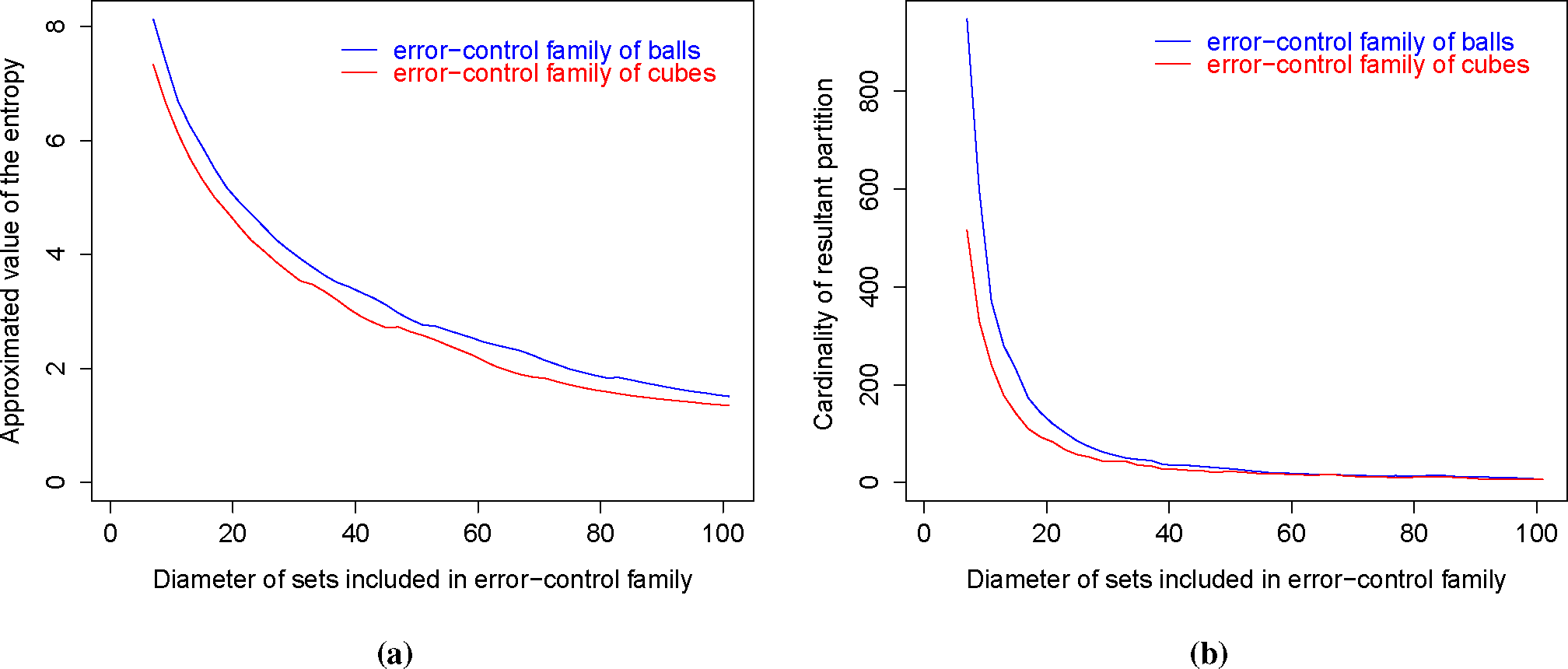
The convergence behavior of the partitions produced by the greedy entropy algorithm was shown in Figure 2. One can observe that the entropy, as well as the cardinality of resultant partitions decrease in a hyperbolic way when the diameters of sets included in the error-control family increase.

1.4. Paper Organization

The paper is organized as follows. In Section 2, we formulate our lossy source coding problem and show that the entropy optimization problem can be simplified by reducing the number of partitions, which are irrelevant for entropy calculation. Section 3 contains our main result. First, the minimum entropy set cover problem is recalled, and its relationship with our notion of entropy is established. Next, we define the greedy entropy algorithm and derive that it constructs a partition with the entropy close to the optimal one.

2. Entropy Calculation

We start this section with establishing basic notations and definitions. Then, we present the main problem of this paper concerning the entropy calculation and show how to reduce its complexity by eliminating irrelevant coding partitions.

2.1. Lossy Source Coding and Error-Control Families

Let us assume that (X, Σ, µ) is a probability space. In our formulation of lossy source coding, we are interested in encoding elements of X produced by a probability measure µ by a countable number of symbols. The source code is determined by a partition of X, which is a countable family of measurable, pairwise disjoint subsets of X, such that:

$$\mu (X\backslash {\displaystyle \underset{P\mathrm{\in }\mathcal{P}}{\cup }\mathcal{P}})=0.$$

More precisely, every element x ∈ X is transformed into a code related to a unique $P\mathrm{\in }\mathcal{P}$, such that x ∈ P. The statistical code length of an arbitrary element of X in the optimal coding scheme can be calculated by the entropy of $\mathcal{P}$[3]:

Definition 1. The entropy of a partition$\mathcal{P}$ is defined by:

$$h(\mu ;\mathcal{P}):={\displaystyle \sum _{P\mathrm{\in }\mathcal{P}}\mathrm{sh}}(\mu (P)),$$

where sh : [0,1] → [0, ∞) is the Shannon function, i.e.,

$$\mathrm{sh}(x):=-x\cdot {\log }_2(x),\mathit{for}x\mathrm{\in }[0,1],$$

where by −0 • log₂(0), we understand zero.

Although the entropy and the partition depend strictly on the probability measure, we consequently omit the symbol µ in their definitions to simplify notations.

The use of a partition causes a coding error (distortion). To be able to control the maximal coding error (the upper limit of permitted distortion), an additional family $\mathcal{Q}$ of subsets of X is introduced, which we call an error-control family [7]. The error-control family restricts the number of permissible partitions that can be used for encoding. More precisely, a partition $\mathcal{P}$ is said to be $\mathcal{Q}$-acceptable iff for every $P\mathrm{\in }\mathcal{P}$, there exists $Q\mathrm{\in }\mathcal{Q}$, such that P ⊂ Q (which we write $\mathcal{P}\prec \mathcal{Q}$).

The partitions that are allowed to be used for encoding are limited by a fixed error-control family. The optimal lossy coding scheme (determined by a partition) is the one that minimizes the entropy and does not violate the upper limit of permitted distortion, i.e., $\mathcal{P}\prec \mathcal{Q}$. This leads to the following definition of the entropy of an error-control family [7].

Definition 2. Let$\mathcal{Q}\subset \sum$ be an error-control family. The entropy of$\mathcal{Q}$ is defined by:

$$H(\mu ;\mathcal{Q}):=\inf \{h(\mu ;\mathcal{P})\mathrm{\in }[0,\infty ]:\mathcal{P}\mathit{\text{is a partiion and}}\mathcal{P}\prec \mathcal{Q}\}.$$

(3)

In this paper, we focus on the computational methods for finding the value of $H(\mu ;\mathcal{Q})$ and possibly a partition $\mathcal{P}\prec \mathcal{Q}$, which satisfies $h(\mu ;\mathcal{P})\approx H\left(\mu ;\mathcal{Q}\right)$. One should look for a partition $\mathcal{P}$ satisfying $h(\mu ;\mathcal{P})=H\left(\mu ;\mathcal{Q}\right)$. However, Example II.1 in [7] shows that the value of entropy does not have to be attained on any partition in general.

2.2. Partition Reduction

In order to find the entropy of an error-control family, a minimization problem (3) has to be solved. Let us first observe that for very simple error-control families, the number of acceptable partitions can be uncountable. Given a family $\mathcal{Q}=\{(-\infty ,1\left]\right[0,+\infty )\}$, any partition of the form $\mathcal{P}=\{(-\infty ,a],(a,\infty )\}$, where a ∈ (0,1), is $\mathcal{Q}$-acceptable. Clearly, some of them do not lead to the optimal solution. As a consequence, it is extremely important to eliminate partitions that are irrelevant for entropy calculation (3).

The main result of this section shows that to find the entropy, it is sufficient to consider only partitions constructed from the sets of ${\mathrm{\Sigma }}_{\mathcal{Q}}$: the σ-algebra generated by the error-control family $\mathcal{Q}$. In the aforementioned example, there are only three such partitions: ${\mathcal{P}}_1=\{(-\infty ,0],(0,+\infty )\}$, ${\mathcal{P}}_2=\{(-\infty ,1],(1,+\infty )\}$ and ${\mathcal{P}}_3=\{(-\infty ,0],(0,1],(1,+\infty )\}$.

Theorem 1. Let (X, Σ, µ) be a probability space, and let$\mathcal{Q}$ be an error-control family. Then, we have:

$$H(\mu ;\mathcal{Q}):=\text{inf}\{h(\mu ;\mathcal{P})\mathrm{\in }\left[0,\infty \right]:\mathcal{P}\mathit{\text{is a partition}},\mathcal{P}\prec \mathcal{Q}\mathit{\text{and}}\mathcal{P}\subset {\mathrm{\Sigma }}_{\mathcal{Q}}\}.$$

To derive this fact, for any $\mathcal{Q}$-acceptable partition $\mathcal{P}$, we will construct a partition $\mathcal{R}\subset {\sum }_{\mathcal{Q}}$ with the entropy not greater than $h(\mu ;\mathcal{P})$. To describe the process of construction of such a partition, let us first establish the notation: for a given partition (or, more generally, family of sets) $\mathcal{P}$ of X and a set A ⊂ X, we denote:

$${\mathcal{P}}_A=\{P\cap A:P\mathrm{\in }\mathcal{P}\}.$$

(4)

This notation will be used through this section.

Then, for a $\mathcal{Q}$-acceptable partition $\mathcal{P}$, a family $\mathcal{R}$ is built by the following Algorithm 1.

Algorithm 1:. Partition reduction algorithm.

Algorithm 1:. Partition reduction algorithm.

Our goal is to show that the partition reduction algorithm produces a partition $\mathcal{R}$, such that:

$$h(\mu ;R)\le h(\mu ;\mathcal{P}).$$

We need to observe that the following property of the Shannon function holds.

Proposition 1. Given numbers p ≥ q ≥ 0 and r > 0, such that p, q,p + r,q − r ∈ [0,1], we have:

$$\mathrm{sh}(p)+\mathrm{sh}(q)\ge \mathrm{sh}(p+r)+\mathrm{sh}(q-r).$$

Let us focus on a single iteration of the partition reduction algorithm.

Lemma 1. Let (X,Σ,µ) be a subprobability space, i.e., (X, Σ) is measurable space, and µ is a non-negative measure on (X, Σ), such that µ(X) ≤ 1. We consider an error-control family$\mathcal{Q}$ and a$\mathcal{Q}$-acceptable partition$\mathcal{P}$ of X. Let$P_{\max }\mathrm{\in }\mathcal{P}$ be such that:

$$\mu (P_{\max })=\max \{\mu (P):P\mathrm{\in }\mathcal{P}\}.$$

If$Q\mathrm{\in }\mathcal{Q}$ is chosen so that P_max ⊂ Q, then:

$$h(\mu ;\{\mathcal{Q}\}\cup {\mathcal{P}}_{X\backslash \mathcal{Q}})\le h(\mu ;\mathcal{P}).$$

(5)

Proof. Clearly, if $h(\mu ;\mathcal{P})=\infty$, then the inequality (5) holds trivially Thus, we assume that $h(\mu ;\mathcal{P})<\infty$.

Let us observe that it is enough to consider only elements of $\mathcal{P}$ with non-zero measures: the number of such sets that can be at most countable. Thus, let us assume that $\mathcal{P}={\left\{P_i\right\}}_{i=1}^{\infty }$ (the case when $\mathcal{P}$ is finite can be treated in a similar manner).

For simplicity, we put P₁ := P_max. For every $k\mathrm{\in }\mathbb{N}$, we consider the sequence of sets, defined by:

$$Q_k:={\displaystyle \underset{i=1}{\overset{k}{\cup }}(P_i\cap Q)}.$$

Clearly, for $k\mathrm{\in }\mathbb{N}$, we have:

$$\begin{array}{c}{Q}_1=P_1,\\ Q_k\subset Q_{k+1},\end{array}$$

$$P_i\cap Q_k=P_i\cap Q,\mathrm{for}i\le k,$$

(6)

$$P_i\cap Q_k=\mathrm{\varnothing },\mathrm{for}i>k,$$

(7)

$$\underset{n\to \infty }{\lim }\mu (Q_n)=\mu (Q).$$

(8)

To complete the proof, it is sufficient to derive that for every $k\mathrm{\in }\mathbb{N}$, we have:

$$h(\mu ;\{Q_k\}\cup {\mathcal{P}}_{X\backslash Q_k})\ge h(\mu ;\{Q_{k+1}\}\cup {\mathcal{P}}_{X\backslash Q_{k+1}})$$

(9)

and:

$$h(\mu ;\{Q_k\}\cup {\mathcal{P}}_{X\backslash Q_k})\ge h(\mu ;\{Q\}\cup {\mathcal{P}}_{X\backslash Q}).$$

(10)

Let $K\mathrm{\in }\mathbb{N}$ be arbitrary. Then, from (6) and (7), we get:

$$\begin{array}{l}h(\mu ;\{Q_k\}\cup {\mathcal{P}}_{X\backslash Q_k})=\mathrm{sh}(\mu (Q_k))+{\displaystyle \sum _{i=2}^{\infty }\mathrm{sh}(\mu (P_i\backslash Q_k))}\\ =\mathrm{sh}(\mu (Q_k))+{\displaystyle \sum _{i=2}^k\mathrm{sh}(\mu (P_i\backslash Q))+{\displaystyle \sum _{i=k+1}^{\infty }\mathrm{sh}(\mu (P_i))}}\\ =h(\mu ;\{Q_{k+1}\}\cup {\mathcal{P}}_{X\backslash Q_{k+1}})+\mathrm{sh}(\mu (Q_k))-\mathrm{sh}(\mu (Q_{k+1}))\\ +\mathrm{sh}(\mu (P_{k+1}))-\mathrm{sh}(\mu (P_{k+1}\backslash \mathcal{Q})).\end{array}$$

Making use of Observation 1, we obtain:

$$\mathrm{sh}(\mu (Q_k))+\mathrm{sh}(\mu (P_{k+1}))\ge \mathrm{sh}(\mu (Q_{k+1}))+\mathrm{sh}(\mu (P_{k+1}\backslash \mathcal{Q})),$$

which proves (9).

To derive (10), we first use Inequality (9). Then:

$$\begin{array}{l}h(\mu ;\{Q_k\}\cup {\mathcal{P}}_{X\backslash Q_k})=\mathrm{sh}(\mu (Q_k))+{\displaystyle \sum _{i=2}^{\infty }\mathrm{sh}(\mu (P_i\backslash Q_k))}\\ \ge \underset{n\to \infty }{\lim }[\mathrm{sh}(\mu (Q_n))+{\displaystyle \sum _{i=1}^{\infty }\mathrm{sh}(\mu (P_i\backslash Q_n))}].\end{array}$$

By (8),

$$\underset{n\to \infty }{\lim }\mathrm{sh}(\mu (Q_n))=\mathrm{sh}(\mu (\mathcal{Q}))<\infty .$$

To calculate $\underset{n\to \infty }{\lim }{\displaystyle {\sum }_{i=1}^{\infty }\mathrm{sh}(\mu (P_i\backslash Q_n))}$, we will use Lebesgue’s dominated convergence theorem [19]. We consider a sequence of functions:

$$f_n:\mathcal{P}∍P\to \mathrm{sh}(\mu (P\backslash Q_n))\mathrm{\in }ℝ,\mathrm{for}n\mathrm{\in }\mathbb{N}.$$

Let us observe that the Shannon function sh is increasing on $[0,2^{-\frac{1}{\ln 2}}]$ and decreasing on $(2^{-\frac{1}{\ln 2}},1]$ Thus, for a certain $m\mathrm{\in }\mathbb{N}$,

$$\mathrm{sh}(\mu (P_i\backslash Q_n))\le 1,\mathrm{for}i\le m$$

and:

$$\mathrm{sh}(\mu (P_i\backslash Q_n))\le \mathrm{sh}(\mu (P_i)),\mathrm{for}i\le m,$$

for every $n\mathrm{\in }\mathbb{N}$. Since $h(\mu ;\mathcal{P})<\infty$, then:

$${\displaystyle \sum _{i=1}^{\infty }\mathrm{sh}(\mu (P_i\backslash Q_n))}\le m+{\displaystyle \sum _{i=m+1}^{\infty }\mathrm{sh}(\mu (P_i))}<\infty .$$

Moreover,

$$\underset{n\to \infty }{\lim }\mathrm{sh}(\mu (P\backslash Q_n))=\mathrm{sh}(\mu (P\backslash Q)).$$

for every $P\mathrm{\in }\mathcal{P}$.

As the sequence of functions ${\{\mathrm{sh}(\mu (P\backslash Q_n))\}}_{n\mathrm{\in }\mathbb{N}}$ satisfies the assumptions of Lebesgue’s dominated convergence theorem [19], then we get:

$$\begin{array}{r}\underset{n\to \infty }{\lim }{\displaystyle \sum _{i=1}^{\infty }\mathrm{sh}(\mu (P_i\backslash Q_n))=}{\displaystyle \sum _{i=1}^{\infty }\underset{n\to \infty }{\lim }\mathrm{sh}(\mu (P_i\backslash Q_n))}\\ ={\displaystyle \sum _{i=1}^{\infty }\mathrm{sh}(\mu (P_i\backslash \mathcal{Q}))<\infty .}\end{array}$$

Consequently, we have:

$$\begin{array}{l}h(\mu ;\{Q_k\}\cup {\mathcal{P}}_{X\backslash Q_k})\ge \underset{n\to \infty }{\lim }[\mathrm{sh}(\mu (Q_n))+{\displaystyle \sum _{i=1}^{\infty }\mathrm{sh}(\mu (P_i\backslash Q_n))}]\\ =\mathrm{sh}(\mu (Q))+{\displaystyle \sum _{i=1}^{\infty }\mathrm{sh}(\mu (P_i\backslash Q))}\\ =h(\mu ;\{Q\}\cup {\mathcal{P}}_{X\backslash Q}),\end{array}$$

which completes the proof. □

Making use of the above lemma, we summarize the analysis of the partition reduction algorithm in the following theorem.

Theorem 2. We assume that (X, Σ, µ) is a subprobability space. Let$\mathcal{Q}$ be an error-control family on X, and let$\mathcal{P}$ be a$\mathcal{Q}$-acceptable partition of X. A family$\mathcal{R}$ constructed by the partition reduction algorithm is a partition of X and satisfies:

$$h(\mu ;\mathcal{R})\le h(\mu ;\mathcal{P}).$$

(11)

Proof. Directly from the partition reduction algorithm, we get that $\mathcal{R}$ is a countable family of pairwise disjoint sets. The fact that:

$$\mu (X\backslash {\displaystyle \underset{R\mathrm{\in }R}{\cup }R})=0,$$

follows from Lebesgue’s dominated convergence theorem [19] applied to a sequence of functions $f_n:\mathcal{P}\to ℝ$ defined by:

$$f_n(P):=\mu (P\backslash {\displaystyle \underset{i=1}{\overset{n}{\cup }}{R}_i}),\mathrm{for}P\mathrm{\in }\mathcal{P}.$$

We prove the inequality (11). If $h(\mu ;\mathcal{P})=\infty$, then the inequality (11) is straightforward. Thus, let us discuss the case when $h(\mu ;\mathcal{P})<\infty$

We denote $\mathcal{P}={\left\{P_i\right\}}_{i=1}^{\infty }$, since at most, a countable number of elements of the partition can have a positive measure (the case when

Directly from Lemma 1, we obtain:

$$h(\mu ;{\mathcal{P}}_{X_k})\ge h(\mu ;{\mathcal{P}}_{X_{k+1}}\cup \{R_k\}),\mathrm{for}k\mathrm{\in }\mathbb{N}.$$

Consequently, for every $k\mathrm{\in }\mathbb{N}$, we get:

$$h(\mu ;{\displaystyle \underset{i=1}{\overset{k}{\cup }}\left\{R_i\right\}\cup {\mathcal{P}}_{X_k}})\ge h(\mu ;{\displaystyle \underset{i=1}{\overset{k+1}{\cup }}\left\{R_i\right\}\cup {\mathcal{P}}_{X_{k+1}}}).$$

(12)

Our goal is to show that:

$$h(\mu ;{\displaystyle \underset{i=1}{\overset{k}{\cup }}\left\{R_i\right\}\cup {\mathcal{P}}_{X_k}})\ge h(\mu ;\mathcal{R}),$$

for every $k\mathrm{\in }\mathbb{N}$.

Making use of (12), we have:

$$\begin{array}{l}h(\mu ;{\displaystyle \underset{i=1}{\overset{k}{\cup }}\left\{R_i\right\}\cup {\mathcal{P}}_{X_k}})={\displaystyle \sum _{i=1}^k\mathrm{sh}(\mu (R_i))}+{\displaystyle \sum _{i=1}^{\infty }\mathrm{sh}(\mu (P_i\backslash {\displaystyle \underset{j=1}{\overset{k}{\cup }}{R}_j))}}\\ \ge \underset{n\to \infty }{\lim }[{\displaystyle \sum _{i=1}^n\mathrm{sh}(\mu (R_i))+{\displaystyle \sum _{i=1}^{\infty }\mathrm{sh}(\mu (P_i\backslash {\displaystyle \underset{j=1}{\overset{n}{\cup }}{R}_j))}}]},,\end{array}$$

for every $k\mathrm{\in }\mathbb{N}$.

We will calculate $\underset{n\to \infty }{\lim }{\displaystyle \sum _{i=1}^{\infty }\mathrm{sh}(\mu (P_i\backslash {\displaystyle \underset{j=1}{\overset{n}{\cup }}{R}_j}))}$ using Lebesgue’s dominated convergence theorem [19] for a sequence of functions ${\left\{f_n\right\}}_{n=1}^{\infty }$, defined by:

$$f_n:\mathcal{P}∍\mathcal{P}\to \mathrm{sh}(\mu (P\backslash {\displaystyle \underset{j=1}{\overset{n}{\cup }}{R}_j}))\mathrm{\in }ℝ,\mathrm{for}n\mathrm{\in }\mathbb{N}.$$

Similar reasoning was used in the proof of Lemma 1.

Similarly to the proof of Lemma 1, we may assume that there exists $m\mathrm{\in }\mathbb{N}$, such that:

$$\mathrm{sh}(\mu (P_i\backslash {\displaystyle \underset{j=1}{\overset{n}{\cup }}{R}_j}))<1,\mathrm{for}i\le m$$

and:

$$\mathrm{sh}(\mu (P_i\backslash {\displaystyle \underset{j=1}{\overset{n}{\cup }}{R}_j}))<\mathrm{sh}(\mu (P_i)),\mathrm{for}i>m,$$

for every $n\mathrm{\in }\mathbb{N}$. Moreover,

$$\underset{n\to \infty }{\lim }\mathrm{sh}(\mu (P\backslash {\displaystyle \underset{j=1}{\overset{n}{\cup }}{R}_j}))=\mathrm{sh}(\mu (P\backslash {\displaystyle \underset{j=1}{\overset{\infty }{\cup }}{R}_j}))=0,$$

for every $P\mathrm{\in }\mathcal{P}$, since $\mathcal{R}$ is a partition of X.

Making use of Lebesgue’s dominated convergence theorem [19], we get:

$$\underset{n\to \infty }{\lim }{\displaystyle \sum _{i=1}^{\infty }\mathrm{sh}(\mu (P_i\backslash {\displaystyle \underset{j=1}{\overset{n}{\cup }}{R}_j}))}={\displaystyle \sum _{i=1}^{\infty }\mathrm{sh}(\mu (P_i\backslash {\displaystyle \underset{j=1}{\overset{\infty }{\cup }}{R}_j}))}=0.$$

Consequently, for every $k\mathrm{\in }\mathbb{N}$, we have:

$$\begin{array}{c}h(\mu ;{\displaystyle \underset{i=1}{\overset{k}{\cup }}\left\{R_i\right\}}\cup {\mathcal{P}}_{X_k})\ge \underset{n\to \infty }{\lim }[{\displaystyle \sum _{i=1}^n\mathrm{sh}(\mu (R_i))}+{\displaystyle \sum _{i=1}^{\infty }\mathrm{sh}(\mu (P_i\backslash {\displaystyle \underset{j=1}{\overset{n}{\cup }}{R}_j}))}]\\ ={\displaystyle \sum _{i=1}^{\infty }\mathrm{sh}(\mu (R_i))}=h(\mu ;R),\end{array}$$

which completes the proof. □

As a consequence of Theorem 2, we directly get that Theorem 1 holds. In the case of finite error-control families, we get that there exists an acceptable partition with minimal entropy.

Corollary 1. Let (X, Σ, µ) be a probability space, and let$\mathcal{Q}$ be a finite error-control family. Then, there exists a$\mathcal{Q}$-acceptable partition$\mathcal{P}\subset {\mathrm{\Sigma }}_{\mathcal{Q}}$, such that:

$$H(\mu ;\mathcal{Q})=h(\mu ;\mathcal{P}).$$

3. Entropy Approximation

In the previous section, we simplified the problem of entropy calculation by reducing the number of partitions that are necessary to consider to find the entropy of an error-control family Since the number of acceptable partitions grows exponentially with the cardinality of the error-control family, it might be impossible to test all of them for entropy calculation. In this section, we show an algorithm that allows us to approximate the entropy within an additive term.

The presented formulation of lossy source coding is closely related to the minimum entropy set cover problem (MESC) [17,18], where one focuses on a similar optimization problem. There exists an algorithm for approximation of the solution of MESC within an additive term of log₂ e. First, we present a description of MESC and its relationship with the introduced coding problem. Next, we use these facts to apply a similar technique for approximating the entropy of an error-control family.

3.1. Relationship with the Minimum Entropy Set Cover Problem

In order to define MESC, let X = {x₁,…, x_n} be a finite dataset, where every observation x ∈ X appears with a probability p_x. A random source produces a signal from a probability distribution $\{p_{x_1},\dots ,p_{x_n}\}$ and passes it through the noisy channel. Each observation has a type, but due to the noise, we only know that it is one of a given set of types defined by a finite cover $\mathcal{Q}=\{Q_1,\dots ,Q_k\}$ of data space X. We map an observation to a type by defining an assignment $f^{\mathcal{Q}}:X\to \mathcal{Q}$, which is compatible with $\mathcal{Q}$,i.e., $x\mathrm{\in }{f}^{\mathcal{Q}}(x)$ for all x ∈ X.

Let us denote by q_i the probability that the random point is assigned to Q_i:

$$q_i:={\displaystyle \sum _{x\mathrm{\in }{f}^{-1}(Q_i)}{p}_x},\mathrm{for}i=1,\dots ,k.$$

The goal is to find such an assignment that minimizes the entropy of the distribution of the types, i.e.,

$$h(f^{\mathcal{Q}}):={\displaystyle \sum _{i=1}^k\mathrm{sh}(q_i).}$$

Such an optimal assignment is denoted by $f_{\mathit{opt}}^{\mathcal{Q}}$.

MESC is an NP-hard problem (Theorem 1 in [18]). To find an assignment that efficiently approximates the minimal entropy value, a simple greedy algorithm can be used (which we call the greedy MESC algorithm). It relies on the iterative execution of the following steps:

• choose the most probable type $Q_{\max }^i\mathrm{\in }\mathcal{Q},$
• if $x\mathrm{\in }{Q}_{\max }^i$, then assign x to $Q_{\max }^i$, i.e., put $f^{\mathcal{Q}}(x):=Q_{\max }^i$,
• remove from X (and from all $Q\mathrm{\in }\mathcal{Q}$) the elements of $Q_{\max }^i$,

until there exists $Q\mathrm{\in }\mathcal{Q}$ with a positive probability [18].

Cardinal et al. proved a sharp bound for the entropy of assignment constructed with the use of the greedy MESC algorithm:

Greedy MESC approximation (see [17] Theorem 1): If $f_g^{\mathcal{Q}}$ is an assignment produced by the greedy algorithm, then:

$$h(f_g^{\mathcal{Q}})\le h(f_{\mathit{opt}}^{\mathcal{Q}})+{\log }_{2}e.$$

To be able to obtain a similar approximation of the entropy of an error-control family, the relationship between MESC and our formulation of entropy has to be established. For this purpose, our lossy source coding problem will be considered on a discrete probability space (X, Σ,µ), where X is a finite set, Σ is a σ-algebra generated by all singletons of X and $\mu :={\displaystyle \sum _{x\mathrm{\in }X}{p}_x{\delta }_x}$ is an atomic measure on (X, Σ). A cover $\mathcal{Q}=\{Q_1,\dots ,Q_k\}$ plays the role of an error-control family

We start our analysis with showing that given an assignment $f^{\mathcal{Q}}$ compatible with $\mathcal{Q}$, one can construct a $\mathcal{Q}$-acceptable partition with equal entropy:

Lemma 2. Let$f^{\mathcal{Q}}$ be an assignment compatible with$\mathcal{Q}$. Then, the family$\mathcal{P}={\left\{P_i\right\}}_{i=1}^k$, where$P_i:={(f^{\mathcal{Q}})}^{-1}(Q_i),$, is a$\mathcal{Q}$-acceptable partition, and:

$$h(f^{\mathcal{Q}})=h(\mu ;\mathcal{P}).$$

Proof. Directly from the definition of compatible assignment, we get that $\mathcal{P}$ is a $\mathcal{Q}$-acceptable partition of X.

Moreover, let us observe that:

$$\begin{array}{l}h(f^{\mathcal{Q}})={\displaystyle \sum _{i=1}^k\mathrm{sh}(q_i)}\\ ={\displaystyle \sum _{i=1}^k\mathrm{sh}({\displaystyle \sum _{x\mathrm{\in }{f}^{-1}(Q_i)}{p}_x})}\\ ={\displaystyle \sum _{i=1}^k\mathrm{sh}({\displaystyle \sum _{x\mathrm{\in }{P}_i}{p}_x})}\\ ={\displaystyle \sum _{i=1}^k\mathrm{sh}(\mu (P_i))=h(\mu ;\mathcal{P})}.\end{array}$$

The following example illustrates that the natural inverse construction is not possible, i.e., for some $\mathcal{Q}$-acceptable partitions, there does not exist any compatible assignment with identical entropy

Example 2. Let (X, Σ, µ) be a probability space with an error-control family$\mathcal{Q}$, where:

$$\begin{array}{c}X=\{0,1\},\\ \sum =\{\mathrm{\varnothing },\{0\},\{1\},\{0,1\left\}\right\},\\ \mu (\{0\})=\mu (\{1\})=\frac{1}{2},\\ \mathcal{Q}=\left\{\right\{0,1\left\}\right\}.\end{array}$$

Then:

$$\mathcal{P}=\left\{\right\{0\},\{1\left\}\right\}$$

is a$\mathcal{Q}$-acceptable partition with the entropy equal to one. However, there is no compatible assignments with the entropy of one: the only assignment$f^{\mathcal{Q}}:X\to \mathcal{Q}$ compatible with$\mathcal{Q}$ is defined by:

$$f^{\mathcal{Q}}(0)=f^{\mathcal{Q}}(1)=\{0,1\},$$

which entropy equal to zero.

The following result demonstrates that given a partition, one can find an assignment without greater entropy:

Lemma 3. Let$\mathcal{P}\prec \mathcal{Q}$ be a partition. Then, there exists an assignment$f^{\mathcal{Q}}$ compatible with$\mathcal{Q}$, such that:

$$h(f^{\mathcal{Q}})\le h(\mu ;\mathcal{P}).$$

Proof. Since $\mathcal{P}$ is a partition, the function:

$$g:X∍x\to {\mathcal{P}}_x\mathrm{\in }\mathcal{P},\mathrm{for}x\mathrm{\in }{\mathcal{P}}_x,$$

is well defined. Moreover, as $\mathcal{P}$ is $\mathcal{Q}$-acceptable, we find a mapping $\mathcal{P}\to \mathcal{Q}$, such that:

$$h(P)=Q,\mathrm{if}P\subset Q.$$

Finally, we put an assignment $f^{\mathcal{Q}}:X\to \mathcal{Q}$, by:

$$f^{\mathcal{Q}}=h\circ g.$$

Clearly, $f^{\mathcal{Q}}$ is an assignment compatible with $\mathcal{Q}$. Let us calculate the entropy of $f^{\mathcal{Q}}$. We have:

$$\begin{array}{l}h(f^{\mathcal{Q}})={\displaystyle \sum _{\mathcal{Q}\mathrm{\in }\mathcal{Q}}\mathrm{sh}({\displaystyle \sum _{x\mathrm{\in }{(f^{\mathcal{Q}})}^{-1}(Q)}{p}_x})}\\ ={\displaystyle \sum _{\mathcal{Q}\mathrm{\in }\mathcal{Q}}\mathrm{sh}({\displaystyle \sum _{x\mathrm{\in }{g}^{-1}(h^{-1}(Q))}{p}_x})}\\ ={\displaystyle \sum _{\mathcal{Q}\mathrm{\in }\mathcal{Q}}\mathrm{sh}({\displaystyle \sum _{\mathcal{P}\mathrm{\in }{h}^{-1}(Q)}{\displaystyle \sum _{x\mathrm{\in }{g}^{-1}(P)}{p}_x}})}.\end{array}$$

Making use of the subadditivity of the Shannon function, we get:

$$\begin{array}{l}{\displaystyle \sum _{Q\mathrm{\in }\mathcal{Q}}\mathrm{sh}({\displaystyle \sum _{P\mathrm{\in }{h}^{-1}(Q)}{\displaystyle \sum _{x\mathrm{\in }{g}^{-1}(P)}{p}_x}})}\le {\displaystyle \sum _{Q\mathrm{\in }\mathcal{Q}}{\displaystyle \sum _{P\mathrm{\in }{h}^{-1}(Q)}\mathrm{sh}({\displaystyle \sum _{x\mathrm{\in }{g}^{-1}(P)}{p}_x}})}\\ ={\displaystyle \sum _{P\mathrm{\in }\mathcal{P}}\mathrm{sh}({\displaystyle \sum _{x\mathrm{\in }{g}^{-1}(P)}{p}_x})}={\displaystyle \sum _{P\mathrm{\in }\mathcal{P}}\mathrm{sh}({\displaystyle \sum _{x\mathrm{\in }\mathcal{P}}{p}_x})}=h(\mu ;\mathcal{P}).\end{array}$$

As a consequence, we get that the entropy of the optimal assignment equals the entropy of an error-control family.

Theorem 3. We have:

$$h(f_{\mathit{opt}}^{\mathcal{Q}})=H(\mu ;\mathcal{Q}).$$

Proof. If $f_{\mathit{opt}}^{\mathcal{Q}}$ is an optimal assignment, then making use of Lemma 2, we construct a $\mathcal{Q}$-acceptable partition $P_1$ that satisfies:

$$h(f_{\mathit{opt}}^{\mathcal{Q}})=h(\mu ;P_1).$$

On the other hand, since $\mathcal{Q}$ is a finite error-control family, then from Theorem 1, we get:

$$H(\mu ;\mathcal{Q})=h(\mu ;{\mathcal{P}}_2),$$

for a specific $\mathcal{Q}$-acceptable partition ${\mathcal{P}}_2$. Using Lemma 3, we find an assignment $f^{\mathcal{Q}}$ compatible with $\mathcal{Q}$, such that:

$$h(\mu ;{\mathcal{P}}_2)\ge h(f^{\mathcal{Q}}),$$

which completes the proof.

3.2. Greedy Approximation

In this section, we show that the analogue of the greedy MESC algorithm can be applied for the case of our formulation of lossy source coding. Furthermore, similar bounds can be established.

Let us start with an extended version of the approximation algorithm, which we call the greedy entropy algorithm (Algorithm 2). Contrary to the greedy MESC algorithm, our procedure works directly with partitions; hence, it is more general. We assume that $\mathcal{Q}$ is a finite error-control family.

Algorithm 2:. Greedy entropy algorithm.

Algorithm 2:. Greedy entropy algorithm.

To see that the greedy entropy algorithm is not well defined for infinite error-control families, let us consider the example:

Example 3. Let us consider an open segment (0,1) with σ-algebra generated by all Borel subsets of (0,1), Lebesgue measure λ and an error control family, defined by:

$$\mathcal{Q}=\{[a,b]:0<a<b<1\}.$$

There does not exist a set of maximal measure from family$\mathcal{Q}$; hence, the greedy entropy algorithm cannot be applied directly in such a case.

Let us observe that both greedy algorithms create partitions with the same entropies. For this purpose, we denote by ${\mathrm{Greedy}}_{\mathcal{Q}}^f$ a set of all assignments produced by the greedy MESC algorithm, while by ${\mathrm{Greedy}}_{\mathcal{Q}}$, we denote a set of all partitions returned by the greedy entropy algorithm:

Proposition 2. We have:

• For every$f_g^{\mathcal{Q}}\mathrm{\in }{\mathrm{Greedy}}_{\mathcal{Q}}^f$, there exists${\mathcal{P}}_g\mathrm{\in }{\mathrm{Greedy}}_{\mathcal{Q}}$, such that:

  $$h(f_g^{\mathcal{Q}})=h(\mu ;{\mathcal{P}}_g).$$
• For every${\mathcal{P}}_g\mathrm{\in }{\mathrm{Greedy}}_{\mathcal{Q}}$, there exists$f_g^{\mathcal{Q}}\mathrm{\in }{\mathrm{Greedy}}_{\mathcal{Q}}^f$, such that:

  $$h(\mu ;{\mathcal{P}}_g)=h(f_g^{\mathcal{Q}}).$$

The main result of this section shows that the greedy entropy algorithm produces a partition with the entropy not greater that the entropy of an error-control family

Theorem 4. Let (X, Σ, µ) be a probability space, and let$\mathcal{Q}$ be a finite error-control family. Then:

$$h(\mu ;\mathcal{P})\le H(\mu ;\mathcal{Q})+{\log }_{2}e,for\mathcal{P}\mathrm{\in }{\mathrm{Greedy}}_{\mathcal{Q}}.$$

The proof of Theorem 4 involves two facts:

• To calculate the entropy, it is sufficient to consider only partitions constructed from the elements of σ-algebra generated by $\mathcal{Q}$ (see Corollary 1).
• The calculation of the entropy of an error-control family is closely related to MESC optimization problem (see Theorem 3 and Proposition 2).

To be able to apply these facts, we need an additional lemma:

Lemma 4. Let (X, Σ,µ) be an arbitrary (not necessarily discrete) probability space, and let$\mathcal{Q}$ be a finite error-control family. Then, there exists a probability space$(\tilde{X},\tilde{\mathrm{\Sigma }},\tilde{\mu })$ with an error-control family$\tilde{\mathcal{Q}}$, such that$\tilde{X}$, $\tilde{\sum }$ and$\tilde{\mathcal{Q}}$ are finite, $\tilde{\mu }$ is an atomic measure,

$$H(\mu ;\mathcal{Q})=H(\tilde{\mu };\tilde{\mathcal{Q}})$$

and for every${\mathcal{P}}_g\mathrm{\in }{\mathrm{Greedy}}_{\mathcal{Q}}$, there exists${\tilde{\mathcal{P}}}_g\mathrm{\in }{\mathrm{Greedy}}_{\tilde{\mathcal{Q}}}$ satisfying:

$$h(\mu ;{\mathcal{P}}_g)=h(\tilde{\mu };{\tilde{\mathcal{P}}}_g).$$

Proof. We restrict our consideration to partitions $\mathcal{P}\subset {\mathrm{\Sigma }}_{\mathcal{Q}}$, since, by Corollary 1, the entropy $H(\mu ;\mathcal{Q})$ is attained on some partition generated by ${\mathrm{\Sigma }}_{\mathcal{Q}}$. Let us denote the set of generators of ${\mathrm{\Sigma }}_{\mathcal{Q}}$:

$$\begin{array}{l}\mathrm{Gen}({\mathrm{\Sigma }}_{\mathcal{Q}}):=\{G\mathrm{\in }{\mathrm{\Sigma }}_{\mathcal{Q}}:G\ne \mathrm{\varnothing },\text{and for all}\\ {\mathcal{Q}}^{\prime }\mathrm{\in }\mathcal{Q}:G\subset Q^{\prime }\mathrm{or}G\cap Q^{\prime }=\mathrm{\varnothing }\}.\end{array}$$

Next, for every set $G\mathrm{\in }\mathrm{Gen}({\mathrm{\Sigma }}_{\mathcal{Q}})$, we fix exactly one point x_G ∈ G.

Then, we obtain a probability space $(\tilde{X},\tilde{\mathrm{\Sigma }},\tilde{\mu })$ and an error-control family $\tilde{\mathcal{Q}}$ by:

$$\begin{array}{c}\tilde{X}=\{x_G{\}}_{G\mathrm{\in }\mathrm{Gen}({\sum }_{\mathcal{Q}})}\\ \tilde{\mathcal{Q}}:=\{{\displaystyle \underset{G\mathrm{\in }\mathrm{Gen}({\sum }_{\mathrm{Q}}),G\subset Q}{\cup }\{x_G\}}{\}}_{Q\mathrm{\in }\mathcal{Q}}\\ \tilde{\sum }={\sum }_{\tilde{\mathcal{Q}}}\\ \tilde{\mu }={\displaystyle \sum _{G\mathrm{\in }\mathrm{Gen}({\sum }_{\mathcal{Q}})}\mu (G){\delta }_{x_G}.}\end{array}$$

It is easy to see that every $\tilde{\mathcal{Q}}$-acceptable $\tilde{\mu }$-partition $\tilde{\mathcal{P}}\subset {\sum }_{\tilde{\mathcal{Q}}}$ corresponds naturally to a specific $\mathcal{Q}$-acceptable partition $\mathcal{P}\subset {\sum }_{\mathcal{Q}}$ and conversely The measures of corresponding sets are equal.

Thus:

$$H(\mu ;\mathcal{Q})=H(\tilde{\mu };\tilde{\mathcal{Q}}).$$

Moreover, for every ${\mathcal{P}}_g\mathrm{\in }{\mathrm{Greedy}}_{\mathcal{Q}}$, there exists ${\tilde{\mathcal{P}}}_g\mathrm{\in }{\mathrm{Greedy}}_{\tilde{\mathcal{Q}}}$, which satisfies:

$$h(\mu ;{\mathcal{P}}_g)=h(\tilde{\mu };{\tilde{\mathcal{P}}}_g).$$

Finally, the proof of our main result is as follows:

Proof. (of Theorem 4) Making use of Lemma 4, we find a probability space $(\tilde{X},\tilde{\mathrm{\Sigma }},\tilde{\mu })$ with the error-control family $\tilde{\mathcal{Q}}$, such that $\tilde{X}$, $\tilde{\sum }$, $\tilde{\mathcal{Q}}$ are finite, $\tilde{\mu }$ is an atomic measure and:

$$H(\mu ;\mathcal{Q})=H(\tilde{\mu };\tilde{\mathcal{Q}}).$$

By Theorem 3, we get that if $f_{\mathit{opt}}^{\tilde{\mathcal{Q}}}$ is an optimal assignment compatible with $\tilde{\mathcal{Q}}$, then:

$$h(f_{\mathit{opt}}^{\tilde{\mathcal{Q}}})=H(\tilde{\mu },\tilde{\mathcal{Q}}).$$

Moreover, making use of Proposition 2, for every ${\tilde{\mathcal{P}}}_g\mathrm{\in }{\mathrm{Greedy}}_{\tilde{\mathcal{Q}}}$, we find $f_g^{\tilde{\mathcal{Q}}}\mathrm{\in }{\mathrm{Greedy}}_{\tilde{\mathcal{Q}}}^f$, such that:

$$h(f_g^{\tilde{\mathcal{Q}}})=h(\tilde{\mu },{\tilde{\mathcal{P}}}_g).$$

Thus, by the greedy MESC approximation, we have:

$$h(\tilde{\mu },{\tilde{\mathcal{P}}}_g)\le H(\tilde{\mu };\tilde{\mathcal{Q}})+{\log }_{2}e.$$

Consequently, using Lemma 4, we get:

$$h(\mu ,{\mathcal{P}}_g)\le H(\mu ;\mathcal{Q})+{\log }_{2}e$$

The above approximation cannot be improved. To see this, we use the example from Section 2 of [17] adopted to our situation. Moreover, it is also NP-hard to approximate the entropy within an additive term lower than log2 e (see Theorem 2 of [17]).

4. Conclusion and Future Work

The paper focused on a non-standard type of lossy source coding. In contrast to rate distortion theory, a cover of the source alphabet, which defines a maximal distortion permitted on every element, was introduced. The calculation of the entropy in such a formulation of lossy coding is equivalent to solving the minimum entropy optimization problem, where one would like to find a coding partition compatible with a fixed distortion with minimal entropy. Our results show how to simplify this optimization problem and to find the approximated entropy value. The proposed algorithm is fast, feasible for implementation and produces a partition that has a proven upper bound on accuracy, i.e., the entropy of the returned partition is not higher than log2 e the true entropy value.

In the future, we plan to consider a more general family of entropy functions, including Rényi and Tsallis entropies, which are of great importance in the theory of coding and related problems [6,20,21]. Moreover, there also arises a natural question concerning the compression of n-tuple random variables. More precisely, it is worth investigating how the coding efficiency increases when the larger blocks of source elements are compressed jointly.

References

- Berger, T. Lossy source coding. IEEE Trans. Inf. Theory 1998, 44, 2693–2723. [Google Scholar]
- Gray, R.M.; Neuhoff, D.L. Quantization. IEEE Trans. Inf. Theory 1998, 44, 2325–2383. [Google Scholar]
- Shannon, C.E. A mathematical theory of communication. Bell Syst. Tech. J. 1948, 27, 379–423. [Google Scholar]
- Bottou, L.; Haffner, P.; Howard, P.G.; Simard, P.; Bengio, Y.; LeCun, Y. High quality document image compression with “DjVu”. J. Electron. Imaging 1998, 7, 410–425. [Google Scholar]
- Kieffer, J.C. A survey of the theory of source coding with a fidelity criterion. IEEE Trans. Inf. Theory 1993, 39, 1473–1490. [Google Scholar]
- Śmieja, M. Weighted approach to general entropy function. IMA J. Math. Control Inf. 2014, 32. [Google Scholar] [CrossRef]
- Śmieja, M.; Tabor, J. Entropy of the mixture of sources and entropy dimension. IEEE Trans. Inf. Theory 2012, 58, 2719–2728. [Google Scholar]
- Śmieja, M.; Tabor, J. Rényi entropy dimension of the mixture of measures. Proceedings of 2014 Science and Information Conference, London, UK, 27–29 August 2014; pp. 685–689.
- Berger, T. Rate-Distortion Theory; Wiley: Hoboken, NJ, USA, 1971. [Google Scholar]
- Ortega, A.; Ramchandran, K. Rate-distortion methods for image and video compression. IEEE Signal Process. Mag. 1998, 15, 23–50. [Google Scholar]
- Gray, R.M. Vector quantization. IEEE ASSP Mag. 1984, 1, 4–29. [Google Scholar]
- Nasrabadi, N.M.; King, R.A. Image coding using vector quantization: A review. IEEE Trans. Commun. 1998, 36, 957–971. [Google Scholar]
- Posner, E.C.; Rodemich, E.R. Epsilon entropy and data compression. Ann. Math. Stat. 1971, 42, 2079–2125. [Google Scholar]
- Posner, E.C.; Rodemich, E.R.; Rumsey, J.H. Epsilon entropy of stochastic processes. Ann. Math. Stat. 1967, 38, 1000–1020. [Google Scholar]
- Rényi, A. On the dimension and entropy of probability distributions. Acta Math. Hungar. 1959, 10, 193–215. [Google Scholar]
- Jayant, N.; Johnston, J.; Safranek, R. Signal compression based on models of human perception. Proc. IEEE 1993, 81, 1385–1422. [Google Scholar]
- Cardinal, J.; Fiorini, S.; Joret, G. Tight results on minimum entropy set cover. Algorithmica 2008, 51, 49–60. [Google Scholar]
- Halperin, E.; Karp, R.M. The minimum-entropy set cover problem. Theor. Comput. Sci. 2005, 348, 240–250. [Google Scholar]
- Kingman, J.F.C.; Taylor, S.J. Introduction to measures and probability; Cambridge University Press: Cambridge, UK, 1966. [Google Scholar]
- Bercher, J.F. Source coding with escort distributions and Rényi entropy bounds. Phys. Lett. A 2009, 373, 3235–3238. [Google Scholar] [Green Version]
- Czarnecki, W.M.; Tabor, J. Multithreshold entropy linear classifier: Theory and applications. Expert Syst. Appl. 2015, 42, 5591–5606. [Google Scholar]
Figure 1.
Input image for compression (a) and partitions produced by the greedy entropy algorithm for two cases of error-control families: the first one (b) consists of cubes with a given side length, while the second (c) contains balls with a given radius. For the visualization, only two color components were used: green and blue in (b) and (c).
Figure 2.
Convergence behavior (entropy (a) and cardinality (b)) of the partitions produced by the greedy entropy algorithm for two cases of error control families: the first one consists of cubes with a given side length, while the second contains balls with a given radius. In every case, the diameters of elements included in the error-control family were increased, which caused the decrease of the entropy and the cardinality of resultant partitions.