The Fisher Information as a Neural Guiding Principle for Independent Component Analysis

Abstract

The Fisher information constitutes a natural measure for the sensitivity of a probability distribution with respect to a set of parameters. An implementation of the stationarity principle for synaptic learning in terms of the Fisher information results in a Hebbian self-limiting learning rule for synaptic plasticity. In the present work, we study the dependence of the solutions to this rule in terms of the moments of the input probability distribution and find a preference for non-Gaussian directions, making it a suitable candidate for independent component analysis (ICA). We confirm in a numerical experiment that a neuron trained under these rules is able to find the independent components in the non-linear bars problem. The specific form of the plasticity rule depends on the transfer function used, becoming a simple cubic polynomial of the membrane potential for the case of the rescaled error function. The cubic learning rule is also an excellent approximation for other transfer functions, as the standard sigmoidal, and can be used to show analytically that the proposed plasticity rules are selective for directions in the space of presynaptic neural activities characterized by a negative excess kurtosis.

1. Introduction

Many living systems, such as neurons and neural networks as a whole, are guided by overarching constraints or principles. Energy [1] and metabolic costs [2] for the information processing of the brain act in this context as basic physiological constrains for the evolution of neural systems [3,4], making, e.g., efficient coding [5,6] a viable strategy.

Metabolic costs can be considered as special cases of objective functions [7], which are to be minimized. Objective functions can however be used in many distinct settings; for example, to guide data selection [8] in engineering applications [9] or to guide learning within neural networks in terms of synaptic plasticity rules by minimizing an appropriate combination of moments of the neural activity [10].

Objective functions can also be formulated in terms of the probability distribution of the neural activity [11], allowing the formulation of information theoretical generative functionals for behavior in general [12–16], for neural activity [17,18], for the derivation of neural plasticity rules in terms of maximizing the relative information entropy [19] or the mutual information [20–22], and for variational Bayesian tasks of the brain through free energy minimization [23].

1.1. Combining Objective Functions

A fundamental question in the context of guiding principles for dynamical systems regards the combination of several distinct and possibly competing objective functions. For a survey of optimization in the context of multiple objective functions, see [9]. For discreteness, we start by considering a generic neural model in which the state of the system is determined by the neural activity y_i of neuron i, by the intrinsic parameters $a_i^k={(\widehat{a})}_i^k$ (with k = 1, 2, … indexing the different internal degrees of freedom) of the neurons and by the inter-neural synaptic connectivity matrix w_ij = (ŵ)_ij. Within the objective functional approach, one considers evolution equations:

$$\{\begin{array}{l}{\dot{y}}_i=-\frac{\partial }{\partial y_i}{\mathcal{F}}^{act}(\mathit{y},\widehat{a},\widehat{w})\\ {\dot{a}}_i^k=-\frac{\partial }{\partial a_i^k}{\mathcal{F}}^{int}(\mathit{y},\widehat{a},\widehat{w})\\ {\dot{w}}_{ij}=-\frac{\partial }{\partial w_{ij}}{\mathcal{F}}^{syn}(\mathit{y},\widehat{a},\widehat{w})\end{array}$$

(1)

for the full dynamical neural system, where there is a specific objective function ${\mathcal{F}}^{\alpha }(\mathit{y},\widehat{a},\widehat{w})$ for every class α ∈ {act, int, syn} of dynamical variables. It is important to note that an overarching objective function like:

$${\mathcal{F}}^{act}(\mathit{y},\widehat{a},\widehat{w}+{\mathcal{F}}^{int}(\mathit{y},\widehat{a},\widehat{w})+{\mathcal{F}}^{syn}(\mathit{y},\widehat{a},\widehat{w}),$$

(2)

does generically not exist. In a biological system, each objective function ${\mathcal{F}}^{\alpha }$ may represent a different regulatory mechanism whose coupling occurs only through the biological agent itself [18]. Indeed, how exactly these mechanisms interact in neural systems, when formulated in terms of learning rules for intrinsic and synaptic plasticity, has been subject of study in recent years [19,24]. Furthermore, for a stationary input distribution, such an overarching functional would result in a gradient system having only point attractors, since limit cycles are not possible in gradient systems [25]. Therefore, a formalism aiming to reproduce the wide variety of behaviors found in natural neural systems cannot be formulated as a gradient system of a single overarching objective function.

One needs to keep in mind, however, that it is often not possible to evaluate rigorously gradients of non-trivial objective functions, as in Equation (1). Generating functionals are hence implemented, in many cases, only approximatively. For the case of information theoretical incentives, as considered in the present work, objective functions are, in addition, formulated in terms of time-averaged statistical properties, and the gradient descent can hence be achieved only through a corresponding time average.

1.2. Hebbian Learning in Neural Networks

Within the neurosciences, synaptic plasticity is generally studied under the paradigm of Hebbian learning [26], stating generically that neurons that fire together, wire together. Depending on whether one considers the frequency (also denoted firing rate), or the timing, of spikes, this principle can have different interpretations. In terms of the firing frequency of neurons, Hebbian learning is understood as a strengthening of the synaptic connection between two neurons (known as potentiation) when both neurons have simultaneously a high activity level or a weakening (depression) of the connectivity if the respective periods of high and low activity do not match [10,27]. In the case of spike timing-dependent plasticity (STDP) [28,29], where synaptic modification is expressed as a function of the precise timing of spikes, on the other hand, the principle of Hebbian learning is understood in terms of causality, stating that a directional synaptic connection should be potentiated if two neurons fire in a causal order, and depressed otherwise [30,31].

In the present work, we consider rate-encoding neurons and, therefore, formulate plasticity in terms of an information theoretical measure of the activity distribution, or alternatively, in terms of the moments of this distribution. While the requirement of any such rule with respect to the Hebbian principle of learning will naturally constrain the manifold of learning rules, the particular details of each rule will determine its functionality. Oja’s rule [27], for instance, is tailored to find the first principal component of a multi-dimensional input distribution. The rules we present in this paper, while able to find the first principal component of a distribution under certain conditions, as we show in [32], will generically perform an independent component analysis by selecting directions of maximal non-Gaussianness.

1.3. Instantaneous Single Neuron

In order to concentrate on the generating principle for synaptic plasticity, we consider here a single instantaneous point neuron, defined by an activity level y,

$$y=\mathrm{\sigma }(x-b),\mathrm{\sigma }(z)=\frac{1}{1+e^{-z}},x={\displaystyle \sum _{j=1}^{N_w}{w}_j(y_j-{\overline{y}}_j),}$$

(3)

representing the average firing rate of the neuron, where σ(z) is a monotonically increasing sigmoidal transfer function, denoted in physics as the Fermi function, that converts the total weighed input x (also referred to as the membrane potential of the neuron) into an output activity. N_w represents the number of incoming inputs y_j, which represent in this case either an external input or the activities of other neurons in a network. b is a bias in the neuron’s sensitivity, and ${\overline{y}}_j$ represents the (trailing) average of the input activity, such that only deviations from this average contribute to the integrated input. An objective function for the neural activity is, in this case, not present, and the evolution Equations (1) reduce to:

$$\{\begin{array}{l}\dot{b}=-{\in }_b\frac{\partial }{\partial b}{\mathcal{F}}^{int}(y,b,\mathbf{w})\\ {\dot{w}}_j=-{\in }_w\frac{\partial }{\partial w_j}{\mathcal{F}}^{syn}(y,b,\mathbf{w})\end{array}\text{with}y=\mathrm{\sigma }\left({\displaystyle \sum w_j(y_j-{\overline{y}}_j)-b}\right),$$

(4)

where we are left only with the objective function for the intrinsic ${\mathcal{F}}^{int}$ and for the synaptic ${\mathcal{F}}^{syn}$ plasticity. Here, we have, with ∈_b and ∈_w, separated the adaption rates from the definition of the respective objective functions.

1.4. Information Theoretical Incentives for Synaptic Plasticity

In the context of stochastic information processing systems, tools from information theory, such as the entropy of a given code or the mutual information between input and output [8], permit one to formulate objective functions for learning and plasticity in terms of the probability distributions of the stochastic elements that constitute the system [6,10–12,14,18,19]. Principles such as maximizing the output entropy of a system to improve the representational richness of the code [19], maximal information transmission for signal separation and deconvolution in networks [33] or maximal predictive information within the sensorimotor loop as a guiding principle to generate behavior [34], have proven successful in the past in both generating new approaches to learning and plasticity and in furthering the understanding of already available rules, integrating them into a broader context by formulating them in terms of a guiding principle [10].

In the present work, we discuss a novel synaptic plasticity rule [32] resulting in self-limiting Hebbian learning and its interaction with known forms of intrinsic plasticity [19,35]. The novelty of this approach relies on the objective function employed, which can be derived from the Fisher information [36] of the output probability distribution with respect to a synaptic flux operator, as shown in Section 2.3. In previous work [32,37], we had shown numerically how a non-linear point neuron employing the Fermi function or the inverse tangent as its transfer function from membrane potential to output activity was able to find the first principal component of an ellipsoidal input distribution, but showed a preference for directions of large negative excess kurtosis otherwise. In the present work, however, we show how, by use of the rescaled error function as a transfer function y(x) = σ(x−b), the resulting learning rule, while qualitatively equivalent to the ones previously studied, takes the form of a simple cubic polynomial in the membrane potential x. This fact, as we will show, represents an important step forward, since it allows us to study the attractors of the learning procedure and their stability analytically. In particular, the rule is shown to have interesting properties in terms of the moments of the input distributions, resulting in a useful tool for independent component analysis, which is thought to be of high relevance for biological cognitive systems [27,38,39].

It is worth mentioning at this point that, while the Fisher information is usually associated with the task of parameter estimation via the Cramér–Rao bound [40–42], it generically encodes the sensitivity of a probability distribution with respect to a given parameter, making it also a useful tool, both in the context of optimal population codes [43–45], or as here, for the formulation of objective functions. Indeed, this procedure has been successfully employed in the past in other fields, to derive, for instance, the Schrödinger equation in quantum mechanics [46].

We will start in the following, as illustrated in Figure 1, with the primary objective function ${\mathcal{F}}^{syn}$ for synaptic plasticity, discussing its relation with the Fisher information for the synaptic flux later on in Section 2.3. Simulation results of the synaptic adaption rules will then be presented in Section 3, in comparison with the results obtained using an analytically-treatable cubic approximation in the membrane potential, as presented in Section 2.1.

2. Objective Functions for Synaptic Plasticity

Our primary objective function for synaptic plasticity is [32]:

$${\mathcal{F}}^{syn}=E\left[{\left(N+x(1-2y)\right)}^2\right],$$

(5)

where E[.] denotes the expected value with respect to the input probability distribution, which can be equated to a time-average whenever the input probability distributions are stationary. The objective function ${\mathcal{F}}^{syn}$ can be expressed entirely in terms of either x or y, which are related by Equation (3). The current form Equation (5) is chosen just for clarity. In Section 2.3, we show how ${\mathcal{F}}^{syn}$ can be derived from the Fisher information with respect to an operator denoted as the synaptic flux operator.

From Equation (5), one can derive easily, via stochastic gradient descent, the update rule:

$${\dot{w}}_j={\in }_{w}G(x)H(x)(y_j-{\overline{y}}_j),$$

(6)

with H(x) = −G′(x) and:

$$G(x)=N+x(1-2y(x)),H(x)=(2y(x)-1)+2x(1-y(x))y(x).$$

(7)

N is a parameter that allows one to shift the positions of the roots of G. The synaptic functions G and H can also be entirely expressed either in terms of x or y, as shown in Figure 2. For N = 2, the two synaptic functions are proportional to each other’s derivatives, G(x) = 2y(1 − y)H′(x), viz. they are conjugate to each other [32].

H(y) is an essentially linear function of positive slope throughout most of the activity range of the neuron; see Figure 2a, saturating only for y → 1/0. The product $H(y)(y_j-{\overline{y}}_j)$ constitutes hence the Hebbian part of the plasticity rule (Equation (6)), resulting in an increase of the synaptic weight whenever the input y_j and the output y are correlated.

The plasticity function G(y), however, reverts the sign of the learning rule if the activity level approaches the extremes, y → 1/0, serving hence as a limiting factor. The process hence adapts the synaptic weights over time, such that the the membrane potential x remains close to the roots of G(x). The synaptic weight will consequently also remain finite, making the adaption rules (Equation (6)) self-limiting.

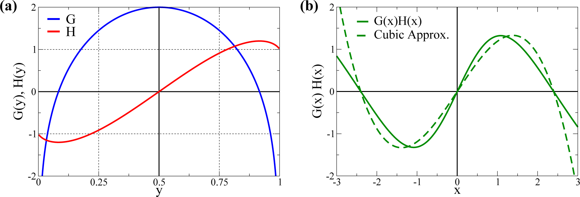
2.1. Cubic Approximation

In order to describe the stationary solutions of Equation (6) in terms of the moments of the input probability distributions, we consider a polynomial expansion in x. The two roots ±x₀ of the limiting function G(x) (compare Figure 2a) are symmetric for the case b = 0, considered in the following, and scale ∼ N for large N [32]. The Hebbian function H(x) has, on the other hand, only a single root at x = 0 (viz at y = 0.5), for b = 0. We are then led to the cubic approximation:

$$\begin{array}{l}{\dot{w}}_j={\mathit{\in }}_{w}G(x)H(x)(y_j-{\overline{y}}_j),\approx -{\mathit{\in }}_{w}x(x-x_0)(x+x_0)(y_j-{\overline{y}}_j)/N^2\\ ={\mathit{\in }}_{w}x(x_0^2-x^2)(y_j-{\overline{y}}_j)/N^2\end{array}$$

(8)

of Equation (6). Note, that the scaling factor 1/N² > 0 could also be absorbed into the adaption rate ∈_w. In Figure 2b, the learning rule from Equation (6) is compared to the cubic approximation (Equation (8)).

For convenience, we denote ${\mathrm{\gamma }}_j=(y_j-{\overline{y}}_j)$, and compute with:

$$\langle {\dot{w}}_j\rangle ={\in }_w\frac{1}{N^2}E\left[{\mathrm{\gamma }}_j\left[\left({\displaystyle \sum _{i=1}^{N_w}{w}_i{\mathrm{\gamma }}_i}\right)x_0^2-{\left({\displaystyle \sum _{i=1}^{N_w}{w}_i{\mathrm{\gamma }}_i}\right)}^3\right]\right],$$

(9)

the time-averaged expectation value of the synaptic weight changes, equating the time average with the statistical average E[.] over the distributions p(y_j) of the input activities y_j. We now assume uncorrelated and symmetric input distributions,

$$E[{\mathrm{\gamma }}_i{\mathrm{\gamma }}_j]=0=E[{\mathrm{\gamma }}_i^k],k=1,3,5,\dots$$

The odd moments hence vanish. Here, it is important to note that any learning rule defined purely in terms of the overall input x = w · γ will be fully rotational invariant. Therefore, the result does not depend on the direction one chooses for the PCs. In particular, if one chooses the principal components to lie along the axes of reference, one can eliminate the linear correlation terms, without loss of generality.

The synaptic weights are quasi-stationary for small adaption rates ∈_w → 0, and we obtain:

$$\langle {\dot{w}}_j\rangle ={\mathit{\in }}_w\frac{1}{N^2}{w}_j{\mathrm{\sigma }}_j^2(x_0^2-w_j^2{\mathrm{\sigma }}_j^2{K}_j-3\mathrm{\Phi })$$

(10)

from Equation (9), where we have defined with:

$${\mathrm{\sigma }}_j^{2}E[{\mathrm{\gamma }}_j^2],K_j=\frac{E[{\mathrm{\gamma }}_j^4]}{{\mathrm{\sigma }}_j^4}-3,\mathrm{\Phi }={\displaystyle \sum _j{w}_j^2{\mathrm{\sigma }}_j^2}$$

(11)

the standard deviation (SD) σ_j of the j-the input, the excess kurtosis K_j and the weighed average Φ of the afferent standard deviations.

2.1.1. Scaling of Dominant Components

The stationary solutions $w_j^{*}$ of Equation (10) satisfy:

$$w_j^{*}=0\vee w_j^{*2}{\mathrm{\sigma }}_j^2{K}_j=x_0^2-3\mathrm{\Phi },$$

(12)

which implies that there is a competition between small components $w_j^{*}\approx 0$ of the synaptic weight vector and large components.

In [32], the authors trained a neuron with ellipsoidal distributions, consisting of normal distributions truncated to [0, 1], with one direction having a large SD σ₁ (the first principal component, or FPC) and the rest of the directions having a small SD. In this context, the weight vector aligns with the FPC, resulting in one large weight (w₁). All other synaptic weight adapt to small values. Solving Equation (12) for the large component yields:

$$|w_1^{cub}|=\frac{x_0}{{\mathrm{\sigma }}_1\sqrt{K_1+3}}.$$

(13)

We note that the excess kurtosis is bounded from below [47], K ≥ −2 (the probability distribution having the lowest possible excess kurtosis of −2 is the bimodal distribution made of two δ-peaks) and that, consequently, K + 3 > 0.

In Section 3.1, a quantitative comparison between Equation (13) and the numerical result of the learning rule is presented.

2.1.2. Sensitivity to the Excess Kurtosis

We are interested now in examining the stability of the solutions obtained via the cubic approximation, in order to explain why a particular solution could be selected in a given setting and not others. To simplify the computations, we study the case of two competing inputs with standard deviations σ_i and excess kurtosis K_i, for i = 1, 2. Three types of solutions can then, in principle, exist:

$$(0,0),(w_1^{*}\ne 0,0),(w_1^{*}\ne 0,w_2^{*}\ne 0),$$

with the $(0,w_2^{*}\ne 0)$ being the analog of $(w_1^{*}\ne 0,0)$. One can compute the eigenvalues λ_1/2 in each case and evaluate the stability of the fixpoints. A sketch of the fixpoints and their stability is presented in Figure 3.

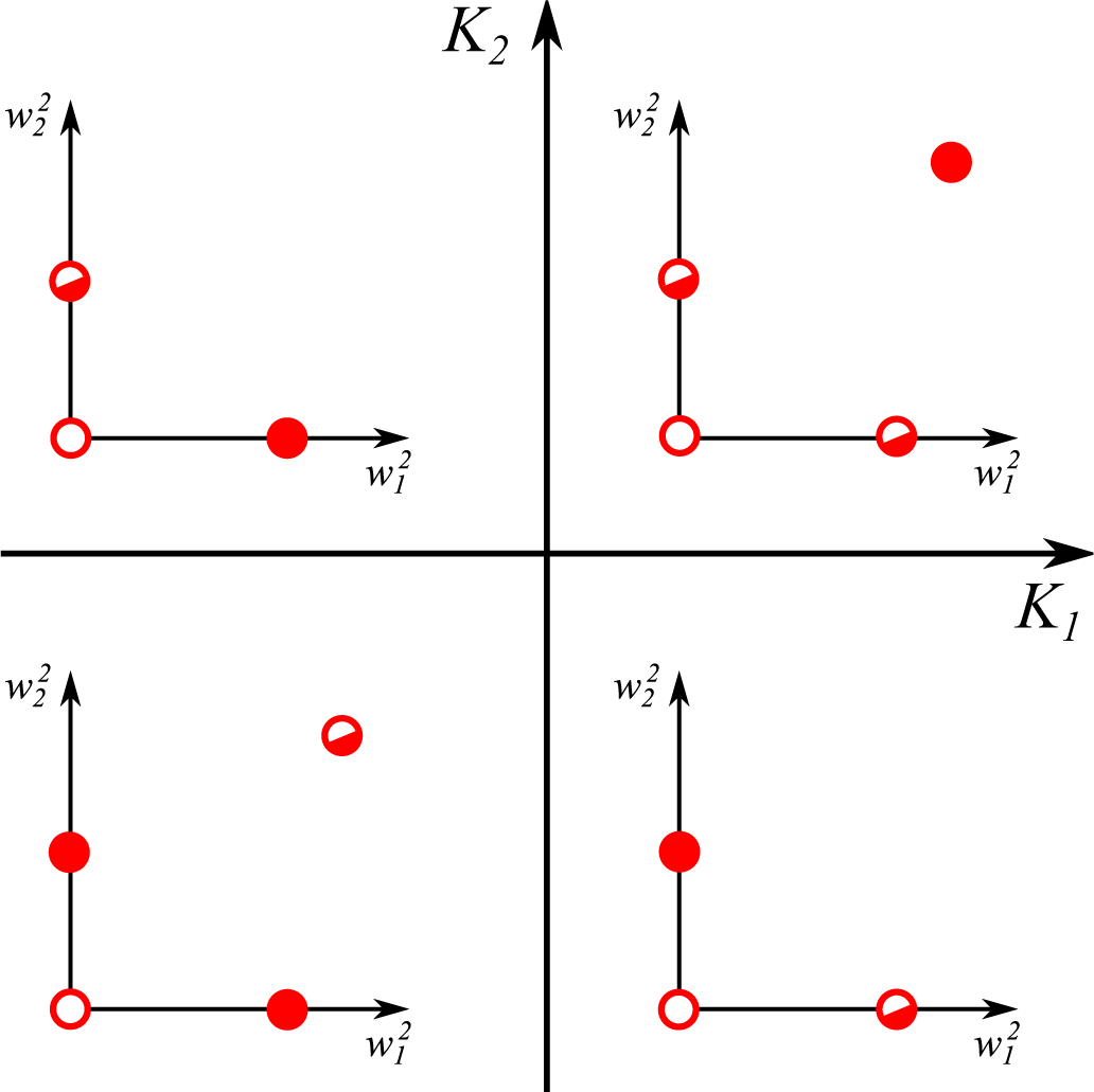
• The trivial fixpoint (0; 0) is always unstable, with positive eigenvalues:

  $${\mathrm{\lambda }}_{1,2}(0,0)={\in }_w\frac{x_0^2}{N^2}({\mathrm{\sigma }}_1^2,{\mathrm{\sigma }}_2^2).$$

  (14)
• For $(w_1^{*}\ne 0,0)$, one finds the eigenvalues:

  $${\mathrm{\lambda }}_{1,2}(w_1^{*}\ne 0,0)={\mathit{\in }}_w\frac{x_0^2}{N^2}\left(-2{\mathrm{\sigma }}_1^2,\frac{{\mathrm{\sigma }}_2^2{K}_1}{K_1+3}\right).$$

  (15)
  The first eigenvalue λ₁ is hence always negative with the sign of the second eigenvalue λ₂ depending exclusively on K₁. The fixpoint $(w_1^{*}\ne 0,0)$ is hence stable/unstable for negative/positive K₁.
• The last term $3\mathrm{\Phi }-x_0^2$ in Equation (12) is identical for all synapses. Two non-zero synaptic weights $(w_1^{*}\ne 0,w_2^{*}\ne 0)$ can hence only exist for identical signs of the respective excess kurtosis, K₁K₂ ≥ 0. It is easy to show that $(w_1^{*}\ne 0,w_2^{*}\ne 0)$ is unstable/stable whenever both K₁,₂ are negative/positive, in accordance with Equation (15).

The solutions of the type $(w_1^{*}\ne 0,0)$ are hence the only stable fixpoints when the excess kurtosis of the corresponding direction, in this case K₁, is negative.

2.1.3. Principal Component Analysis

The observation [32] that the update rules from Equation (6) perform a principal component analysis (PCA) can be understood on two levels.

It is firstly evident from Equation (10) that $\langle {\dot{w}}_j\rangle ~{\mathrm{\sigma }}_j^2$, and that synaptic weight tends hence to grow fast whenever the corresponding presynaptic input has a large variance ${\mathrm{\sigma }}_j^2$.

Alternatively, one can consider the respective phase-space contractions ${\mathrm{\lambda }}_1^{(\alpha )}+{\mathrm{\lambda }}_2^{(\alpha )}$ (see Equation (15)) around the two competing fixpoints ${\mathbf{w}}^{(\alpha =1)}=(w_1^{*}\ne 0,0)$ and ${\mathbf{w}}^{(\alpha =2)}=(w_2^{*}\ne 0,0)$. Using the expression in Equation (15) for the case K₁ = K₂ < 0, one finds that the phase space contracts faster around w⁽¹⁾ when ${\mathrm{\sigma }}_1^2>{\mathrm{\sigma }}_2^2$, and vice versa.

2.2. Alternative Transfer Functions

The objective function from Equation (5) can be expressed generically [37] as:

$${\mathcal{F}}^{syn}=E\left[{(N+A(x))}^2\right],A(x)=\frac{x{y}^{″}}{y^{\prime }},$$

(16)

where y′ and y″ represent the first and second derivative of the transfer function y(x) = σ(x − b) with respect to x. This expression, which appears as an intermediate step in the derivation of the objective function from the Fisher information (compare Section 2.3), reduces to Equation (5) for the sigmoidal transfer function defined in Equation (3).

The qualitative behavior of the learning rule remains unchanged when considering alternative functional forms for the transfer function y(x), whenever they fulfill the basic requirement of being smooth monotonic functions with lim_x→∓∞ y(x) = 0/1. For example, in [37], the authors showed that this is indeed the case for an arc-tangential transfer function. An interesting transfer function to consider in this context is the rescaled error function erf(x − b),

$$y=\frac{1}{2}+\frac{1}{2}\text{erf}\left(\frac{x-b}{s\sqrt{2}}\right)=\frac{1}{2}+\frac{1}{\sqrt{\pi }}{\displaystyle {\int }_{-\infty }^{(x-b)/(s\sqrt{2})}{\mathrm{e}}^{-z^{2}dz}}=\frac{1}{\sqrt{2\pi s}}{\displaystyle {\int }_{-\infty }^{(x-b)}{\mathrm{e}}^{-\frac{z^2}{2s^2}dz}},$$

(17)

as defined by the integral of the normal distribution of variance s. The constant s sets the slope of the transfer function, and if one wants to have the same slope as for the original transfer function (Equation (3)), one simply sets s$s=4/\sqrt{2\pi }$. The derivatives of Equation (17) are:

$$y^{\prime }=\frac{1}{\sqrt{2\pi s}}{\mathrm{e}}^{-\frac{{(x-b)}^2}{2s^2}},y^{″}=\frac{(x-b)}{s^2}{y}^{\prime }.$$

(18)

Using Equation (16), one obtains:

$${\mathcal{F}}^{syn}=E\left[{\left(N-\frac{x(x-b)}{s^2}\right)}^2\right]$$

(19)

for the objective function and, consequently:

$$\begin{array}{l}{\dot{w}}_j={\mathit{\in }}_w(x-b/2)\left(N{s}^2-x(x-b)\right)(y_j-{\overline{y}}_j)\\ ={\mathit{\in }}_w(x-b/2)\left(x_0^2-x(x-b)\right)(y_j-{\overline{y}}_j)\end{array}$$

(20)

for the synaptic plasticity rule, where we have replaced Ns² by $x_0^2$, the squared roots for b = 0. Equation (20) reduces, interestingly and apart from an overall scaling factor, to the cubic approximation from Equation (20) for b = 0:

$${\dot{w}}_j=-{\mathit{\in }}_{w}x(x-x_0)\left(x+x_0\right)(y_j-{\overline{y}}_j)={\mathit{\in }}_{w}x\left(x_0^2-x^2\right)(y_j-{\overline{y}}_j).$$

(21)

For non-vanishing b, we can rewrite Equation (20), as:

$${\dot{w}}_j=-{\mathit{\in }}_w(x-b/2)(x-x^{-})(x-x^{+})(y_j-{\overline{y}}_j).$$

(22)

with:

$$x^{\pm }=-\frac{b}{2}\pm \sqrt{b^2/4+x_0^2}\approx -\frac{b}{2}\pm x_0,$$

(23)

where the last expression holds for small b. The whole learning rule from Equation (21) is therefore, for small bias b, simply shifted by a factor b/2.

Finally, in analogy to Equation (7), we can again write Equation (20) as a product of a Hebbian term (H) and a self-limiting term (G):

$${\dot{w}}_j={\mathit{\in }}_{w}H(x)G(x)(y_j-{\overline{y}}_j),H(x)=(x-b/2),G(x)=(x_0^2-x(x-b)).$$

(24)

In order to compare to Figure 2a, functions G and H, now as defined in Equation (24), are plotted as a function of the activity level y in Figure 4a.

We can now easily compute the average weight change for Equation (20) in the same way we did for Equation (8), obtaining:

$$\langle {\dot{w}}_j\rangle ={\mathit{\in }}_w{w}_j{\mathrm{\sigma }}_j^2\left[\left(x_0^2-\frac{b^2}{2}\right)+\frac{3b}{2}{w}_j{\mathrm{\sigma }}_j{S}_j-w_j^2{\mathrm{\sigma }}_j^2{K}_j-3\mathrm{\Phi }\right],$$

(25)

where S_j is the skewness of input distribution y_j, as defined by:

$$S_j=\frac{E[{\mathrm{\gamma }}_j^3]}{{\mathrm{\sigma }}_j^3}.$$

(26)

In Expression (25), the interaction between intrinsic and synaptic plasticity becomes evident through b. We note that for symmetric input distributions (S_j = 0) as the ones we have been treating, small values of b produce only a shift in the effective x₀ (provided that b² is smaller than $x_0^2/2$).

We note that the trivial solution w_j=0 would become stable for negative $x_0^2-b^2/2$. This has however not happened for the numerical simulations we performed, which resulted in values of b ≈ 1, for target activity levels hyi as low as 0.1, while x₀ = 2.4 for N = 2 (which we used). Even sparser activity levels 〈y〉 as low as 0:1, while x0 = 2:4 for N = 2 (which we used). Even sparser activity levels 〈y〉 ≪1 would require larger firing thresholds b ≫ 1, and stable synaptic plasticity would be achieved be selecting then appropriately large N, corresponding to values of x₀, such that $x_0^2-b^2/2$ remains positive.

For non-symmetric distributions, the skewness of the input distribution, together with the sign of b, will determine the sign w, which was before undetermined, since the learning rules are rotationally invariant.

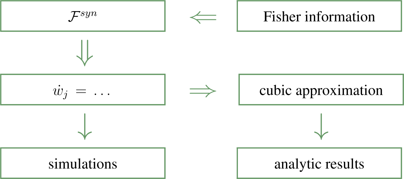
2.3. The Stationarity Principle of Statistical Learning

In statistical learning, one considers an agent trying to extract information from data input streams having stationary statistical properties. In a neural setting, this corresponds to a neuron adapting the afferent synaptic weights, and learning is complete when the synaptic weights do not change any more. At this point, the probability distribution function p(y) of the neural activity y also becomes stationary, and its sensitivity with respect to changes in the afferent synaptic weight vector vanishes. This is the stationarity principle of statistical learning.

2.3.1. The Fisher Information with Respect to the Synaptic Flux

The Fisher information [36]:

$${\mathcal{F}}_0={\displaystyle \int p_0(y){\left(\frac{\partial }{\partial \theta }\ln (p_0(y))\right)}^{2}dy}$$

(27)

encodes the average sensitivity of a given probability distribution p_θ(y) with respect to a certain parameter θ, becoming minimal whenever θ does not influence the statistics of y. The Fisher information is hence a suitable information theoretical functional for the implementation of the stationarity principle of statistical learning.

We drop the index θ in the following and consider in the first step a neuron with N_w = 1 afferent neurons. We define with:entropy-17-03838entropy-17-03838entropy-17-03838

$${\mathcal{F}}_0={\displaystyle \int p_0(y){\left(\frac{\partial }{\partial \theta }\ln (p_0(y))\right)}^{2}dy}$$

(28)

an objective function for synaptic plasticity, measuring the sensibility of the neural activity with respect to the afferent synaptic weight w₁. Here, y(y₁) is given by $\mathrm{\sigma }(w_1(y_1-{\overline{y}}_1)-b)$, as defined in Equation (3). There are two changes with respect to the bare Fisher information (Equation (27)).

• The operator w₁∂/∂w₁ corresponds to a dimensionless differential operator and, hence, to the log-derivative. The whole objective function ${\mathcal{F}}_{N_w=1}^{syn}$ is hence dimensionless.
• The average sensitivity is computed as an average over the probability distribution p(y₁) of the presynaptic activity y₁, since we are interested in minimizing the time average of the sensitivity of the postsynaptic activity with respect to synaptic weight changes in the context of a stationary presynaptic activity distribution p(y₁).

For a distribution p(y(y₁)), for which y is a monotonic function of y₁, we have:

$$p(y(y_1))dy=p(y_1)d{y}_1,p(y(y_1))=\frac{p(y_1)}{\partial y/\partial y_1},$$

(29)

which allows us to rewrite Equation (28) as:

$${\mathcal{F}}_{N_w=1}^{syn}={\displaystyle \int {\left(w_1\frac{\partial }{\partial w_1}\ln \left(\frac{p(y_1)}{\partial y/\partial y_1}\right)\right)}^2}p(y_1)d{y}_1.$$

(30)

Defining with y = (y₁,…, y_Nw) the vector of afferent synaptic weights and with p(y) the corresponding probability distribution function, we may generalize Equation (30) as:

$${\mathcal{F}}_{N_w=1}^{syn}={\displaystyle \int {\left({\displaystyle \sum _{j=1}^{N_w}{w}_j\frac{\partial }{\partial w_j}\ln }\left(\frac{p(y_1)}{\partial y/\partial y_1}\right)\right)}^2}p(\mathit{y})d\mathit{y},$$

(31)

where we have replaced p(y(y)) from Equation (28) by $\frac{p(y_j)}{\partial y/\partial y_j}$, in what constitutes the independent synapse extension, and which represents the Fisher information with respect to the flux operator:

$$\frac{\partial }{\partial \theta }\to {\displaystyle \sum _j{w}_j\frac{\partial }{\partial w_j}=\mathbf{w}\cdot {\nabla }_w,}$$

(32)

which is a dimensionless scalar. We give some comments:

• Minimizing ${\mathcal{F}}_{N_w}^{syn}$, in accordance with the stationarity principle for statistical learning, leads to a synaptic weight vector w that is perpendicular to the gradient ∇_w(log(p)), restricting consequently the overall growth of the modulus of w.
• In ${\mathcal{F}}_{N_w}^{syn}$, there is no direct cross-talk between different synapses. Expression Equation (32) is hence adequate for deriving Hebbian-type learning rules in which every synapse has access only to locally-available information, together with the overall state of the postsynaptic neuron in terms of its firing activity y or its membrane potential x. We call Equation (32) the local synapse extension with respect to other formulations allowing for inter-synaptic cross-talk.
• It is straightforward to show [37] that Equation (31) reduces to Equation (5), when using the relations from Equation (3), viz. ${\mathcal{F}}_{N_w}^{syn}={\mathcal{F}}^{syn}$when we identify N → N_w. We have, however, opted to retain N generically as a free parameter in Equation (5), allowing us to shift appropriately the roots of G(x).

3. Results and Discussion

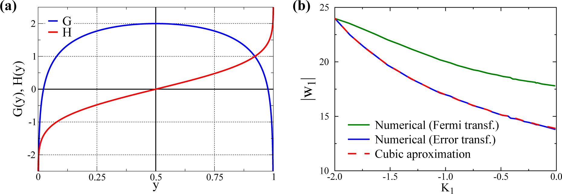
3.1. Quantitative Comparison of the Model and the Cubic Approximation

In the present section, we test the prediction of Equation (13) for the dependence of the weight size on the standard deviation σ_j and kurtosis K_j of the input distribution. Given that the input distribution has a finite width, the integrated input x cannot fall into the minima of the objective function for every point in the distribution, but rather the cloud of x points generated will tend to spread around these minima. The discrepancies in the rule from the cubic approximation in the vicinity and away from the minima are then expected to affect the final result of the learning procedure.

In order to test Equation (13), we use as an input for the direction of the first principal component (FPC, which is chosen to be along y₁, without loss of generality), the sum:

$$\frac{1}{2}\left[N\left(x-\frac{1+2d}{2},{\mathrm{\sigma }}_s\right)+N\left(x-\frac{1-2d}{2},{\mathrm{\sigma }}_s\right)\right]$$

of two normal distributions N(x, σ_s) with individual standard deviations σ_s, whose peaks are at a distance ±d from the center of the input range (0.5).

• σ_s is adjusted, changing d, such that the overall standard deviation σ₁ remains constant. In this way, one can select with d different kurtosis levels, while retaining a constant standard deviation. For d = 0, one gets a bound (since y₁ ∈ [0, 1]) normal distribution with K₁ ≈ 0 (slightly negative, since the distributions are bound). In this way, we can evaluate the size of w₁ after training for a varying K₁ ∈ [−2, 0) for any given σ₁.
• For the other N_w − 1 directions, we use bound normal distributions with standard deviations σ_i = σ₁/2 as in [32].

We tested training the neuron using both the original learning rule (Equation (6)), derived for the Fermi transfer function, and the cubic rule (Equation (20)) for the error function.

In Figure 4b, the value of w₁ after training is presented together with the prediction (Equation (13)) from the cubic approximation, as a function of K₁ (the kurtosis in the y₁ direction), for a constant b = 0. In this case, we have used σ₁ = 0.1 and σ_i≠1 = σ₁/2.

The prediction of the cubic approximation is indeed practically exact for the error transfer function, as expected, since the input distributions are symmetric and, if one sets the axes parallel to the principal components, as we did in this case, the correlation terms indeed vanish, therefore fulfilling the assumptions made during the averaging procedure. Apart from this procedure, no other approximations were made in this case, since the rule for the error function is identical to the cubic approximation in the b = 0 case.

As shown in Figure 2b, even though the cubic approximation is able to reproduce the roots of the learning rule derived for the Fermi transfer function, the cubic approximation grows faster in the outer region, restricting the growth of the synaptic weight more than the original rule would. One therefore expects the cubic approximation to underestimate the final value of w₁, as indeed is observed in Figure 4b. When K = −2, the input distribution becomes the sum of two deltas, and the rule is able to assign each delta to a root. The prediction is of course once again exact in this case. Otherwise, while the quantitative result differs from one rule to another, the qualitative behavior remains unchanged.

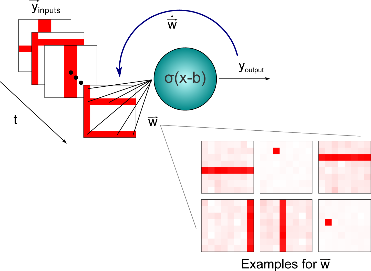
3.2. Independent Component Analysis: An Application to the Nonlinear Bars Problem

Incoming signals may result from the sum of non-Gaussian independent sources, and the process of extracting these sources is denoted independent component analysis (ICA) [48].

The non-Gaussianness of the independent sources may be characterized in principle by any quantity that is zero for the normal distribution and non-zero otherwise. Common measures include the kurtosis K and the skewness S or the negentropy in general. For a comprehensive summary of the principles behind typical ICA procedures, as well as a description of independent components in terms of the cumulative moments of the probability distributions, see [49]. Our learning rule is functionally dependent both on the kurtosis in general, as is evident within the cubic approximation (Equation (10)), and on the skewness for non-zero bias b (Equation (25)) and, hence, prone to perform an ICA. We note, however, that this dependency does not result from maximizing a given measure of non-Gaussianness, as performed in the past by several groups [50,51]. The resulting preference for non-Gaussianness is in the case of the present work a by-product of the stationarity principle of statistical learning. In [27], the author shows how, under certain conditions, a neural network evolving under a nonlinear principal component analysis learning rule, is also capable of performing ICA.

The classical ICA is, strictly speaking, defined only for linear superpositions of sources. One can generalize this concept to non-linear tasks, and we test our multiplicative learning rule (Equation (6)) using a classical example for a non-linear ICA, the non-linear bars problem [35], in which a neuron, or a network of neurons, is trained with a set of inputs, each representing an image consisting on the non-linear superposition of horizontal and vertical bars.

In a grid of N_w inputs where N_w = L × L, each horizontal and vertical bar has a constant probability of being present of p = 1/L. Each input or pixel can take only two values: a low-intensity and a high-intensity value. Each bar then corresponds to a whole row or a column of high-intensity pixels, where at the intersection of two bars, the pixel has the same value (high) as in the rest of the bar, making the problem non-linear.

The here examined synaptic plasticity rules (Equation (6)) are able, as illustrated in Figure 5, to discriminate individual bars, the independent components of the input patterns or points [37]. One might argue that, given that in the original training set of [35] single bars will occur in the training set with a finite probability, the neuron is simply selecting this particular input. To rule out this possibility, we trained the neuron also with sets having at least one horizontal and one vertical bar each time, so that no bar is ever presented in isolation. No appreciable change in the performance was observed.

4. Conclusions

We presented guiding principles for deriving plasticity rules for the synaptic weight of interconnected neurons, which are motivated by considering an information theoretical measure, namely the Fisher information, for the implementation of the stationarity principle of statistical learning. We showed how, in the case of ellipsoidal input distributions, the resulting plasticity rules find, as usual for Hebbian learning, the dominant principal component in the data input stream, when present, being selective otherwise for non-Gaussianness in terms of the excess kurtosis and the skewness of the input activities. The plasticity rules are hence also prone to perform an independent component analysis, as we demonstrated by considering the non-linear bars problem.

The here examined adaption rules are self-limiting. This is a natural consequence of implementing the stationarity principle of statistical learning, which states that the statistics of the postsynaptic neural firing will become stationary whenever learning is complete and when the statistics of the input activity is itself stationary. The self-limitation is achieved through a multiplicative factor to the usual Hebbian-type plasticity function, in contrast to other approaches, where runaway growth of the synaptic weights is avoided by performing either an overall renormalization of the synaptic weights or by adding an explicit weight decay term.

In previous work [32], a numerical comparison between the learning rules here proposed and the traditionally-employed Oja’s rule was performed, showing differences in the sensitivity to higher moments of the input distribution (Oja’s rule is tailored to be sensitive to the second moment of the input distribution only), as well as a stark contrast in terms of transient dynamics. While Oja’s rule predicts the neuron to learn and unlearn the direction of the PCA within the same timescale when a new interesting direction is presented, a fading memory effect is observed when the present rules are employed. We believe then that, depending on the application at hand and the level of noise in the environment, one or the other might prove more suitable.

The objective function from Equation (16) and the learning rules discussed here depend on the specific form y(x) of the transfer function, becoming a cubic polynomial in the membrane potential x when the transfer function is a rescaled error function. This cubic plasticity rule (Equation (20)) is, at the same time, an excellent approximation for the update rule (Equation (6)) valid for sigmoidal transfer functions, allowing one to derive analytically the sensibility of our learning rules to the excess kurtosis, as discussed in Section 2.1.2. The polynomial update rules allow also to study, given its polynomial character, the stability of the learning dynamics quite generally in terms of the moments of the input distribution.

Finally, we have shown here and in [37] how neurons operating under several transfer functions, and with learning rules that are only qualitatively equivalent to the cubic function, are able to perform identical computational tasks. We have also tested whether a neuron defined by one particular transfer function can be trained using the learning rule derived for another choice of sigmoidal function, finding no major changes to the results. The procedure is then very robust to quantitative deviations from the derived rules, as long as the plasticity rule remains qualitatively similar to a cubic polynomial in the membrane potential, an important requirement for biological plausibility.

References

1. Attwell, D.; Laughlin, S.B. An energy budget for signaling in the grey matter of the brain. J. Cereb. Blood Flow Metab. 2001, 21, 1133–1145. [Google Scholar]
2. Mink, J.W.; Blumenschine, R.J.; Adams, D.B. Ratio of central nervous system to body metabolism in vertebrates: its constancy and functional basis. Am. J. Physiol.-Regul. Integr. Comp. Physiol. 1981, 241, R203–R212. [Google Scholar]
3. Niven, J.E.; Laughlin, S.B. Energy limitation as a selective pressure on the evolution of sensory systems. J. Exp. Biol. 2008, 211, 1792–1804. [Google Scholar]
4. Bullmore, E.; Sporns, O. The economy of brain network organization. Nat. Rev. Neurosci. 2012, 13, 336–349. [Google Scholar]
5. Lee, H.; Battle, A.; Raina, R.; Ng, A.Y. Efficient sparse coding algorithms. In Advances in Neural Information Processing Systems: Proceedings of The First 12 Conferences; Jordan, M.I., LeCun, Y., Solla, S.A., Eds.; The MIT Press: Cambridge, MA, USA, 2001; pp. 801–808. [Google Scholar]
6. Stemmler, M.; Koch, C. How voltage-dependent conductances can adapt to maximize the information encoded by neuronal firing rate. Nat. Neurosci. 1999, 2, 521–527. [Google Scholar]
7. Gros, C. Generating functionals for guided self-organization. In Guided Self-Organization: Inception; Prokopenko, M., Ed.; Springer: Berlin/Heidelberg, Germany, 2014; pp. 53–66. [Google Scholar]
8. MacKay, D. Information-based objective functions for active data selection. Neural Comput. 1992, 4, 590–604. [Google Scholar]
9. Marler, R.T.; Arora, J.S. Survey of multi-objective optimization methods for engineering. Struct. Multidiscip. Optim. 2004, 26, 369–395. [Google Scholar]
10. Intrator, N.; Cooper, L.N. Objective function formulation of the BCM theory of visual cortical plasticity: Statistical connections, stability conditions. Neural Netw. 1992, 5, 3–17. [Google Scholar]
11. Kay, J.W.; Phillips, W. Coherent infomax as a computational goal for neural systems. Bull. Math. Biol. 2011, 73, 344–372. [Google Scholar]
12. Polani, D. Information: currency of life. HFSP J 2009, 3, 307–316. [Google Scholar]
13. Zahedi, K.; Ay, N.; Der, R. Higher coordination with less control—A result of information maximization in the sensorimotor loop. Adapt. Behav. 2010, 18, 338–355. [Google Scholar]
14. Polani, D.; Prokopenko, M.; Yaeger, L.S. Information and self-organization of behavior. Adv. Complex Syst. 2013, 16, 1303001. [Google Scholar]
15. Prokopenko, M.; Gershenson, C. Entropy Methods in Guided Self-Organisation. Entropy 2014, 16, 5232–5241. [Google Scholar]
16. Der, R.; Martius, G. The Playful Machine: Theoretical Foundation and Practical Realization of Self-Organizing Robots; Springer: Berlin, Heidelberg, Germany, 2012; Volume 15. [Google Scholar]
17. Markovic, D.; Gros, C. Self-organized chaos through polyhomeostatic optimization. Phys. Rev. Lett. 2010, 105, 068702. [Google Scholar]
18. Marković, D.; Gros, C. Intrinsic adaptation in autonomous recurrent neural networks. Neural Comput. 2012, 24, 523–540. [Google Scholar]
19. Triesch, J. Synergies between intrinsic and synaptic plasticity mechanisms. Neural Comput. 2007, 19, 885–909. [Google Scholar]
20. Linsker, R. Local synaptic learning rules suffice to maximize mutual information in a linear network. Neural Comput. 1992, 4, 691–702. [Google Scholar]
21. Chechik, G. Spike-timing-dependent plasticity and relevant mutual information maximization. Neural Comput. 2003, 15, 1481–1510. [Google Scholar]
22. Toyoizumi, T.; Pfister, J.P.; Aihara, K.; Gerstner, W. Generalized Bienenstock–Cooper–Munro rule for spiking neurons that maximizes information transmission. Proc. Natl. Acad. Sci. USA 2005, 102, 5239–5244. [Google Scholar]
23. Friston, K. The free-energy principle: A unified brain theory. Nat. Rev. Neurosci. 2010, 11, 127–138. [Google Scholar]
24. Mozzachiodi, R.; Byrne, J.H. More than synaptic plasticity: Role of nonsynaptic plasticity in learning and memory. Trends Neurosci. 2010, 33, 17–26. [Google Scholar]
25. Strogatz, S.H. Nonlinear Dynamics and Chaos: With Applications to Physics, Biology and Chemistry; Perseus Publishing: Boulder, CO, USA, 2001. [Google Scholar]
26. Hebb, D.O. The Organization of Behavior: A Neuropsychological Theory; Psychology Press: Mahwah, NJ, USA, 2002. [Google Scholar]
27. Oja, E. The nonlinear PCA learning rule in independent component analysis. Neurocomputing 1997, 17, 25–45. [Google Scholar]
28. Bi, G.Q.; Poo, M.M. Synaptic modifications in cultured hippocampal neurons: Dependence on spike timing, synaptic strength, and postsynaptic cell type. J. Neurosci. 1998, 18, 10464–10472. [Google Scholar]
29. Froemke, R.C.; Dan, Y. Spike-timing-dependent synaptic modification induced by natural spike trains. Nature 2002, 416, 433–438. [Google Scholar]
30. Izhikevich, E.M.; Desai, N.S. Relating stdp to bcm. Neural Comput. 2003, 15, 1511–1523. [Google Scholar]
31. Echeveste, R.; Gros, C. Two-trace model for spike-timing-dependent synaptic plasticity. Neural Comput. 2015, 27, 672–698. [Google Scholar]
32. Echeveste, R.; Gros, C. Generating functionals for computational intelligence: The Fisher information as an objective function for self-limiting Hebbian learning rules. Front. Robot. AI 2014, 1. [Google Scholar] [CrossRef]
33. Bell, A.J.; Sejnowski, T.J. An information-maximization approach to blind separation and blind deconvolution. Neural Comput. 1995, 7, 1129–1159. [Google Scholar]
34. Martius, G.; Der, R.; Ay, N. Information driven self-organization of complex robotic behaviors. PloS ONE 2013, 8, e63400. [Google Scholar]
35. Földiak, P. Forming sparse representations by local anti-Hebbian learning. Biol. Cybern. 1990, 64, 165–170. [Google Scholar]
36. Brunel, N.; Nadal, J.P. Mutual information, Fisher information, and population coding. Neural Comput. 1998, 10, 1731–1757. [Google Scholar]
37. Echeveste, R.; Gros, C. An objective function for self-limiting neural plasticity rules. Proceedings of the 23th European Symposium on Artificial Neural Networks, Computational Intelligence and Machine Learning (ESANN), Bruges, Belgium, 22–24 April 2015.
38. Hyvärinen, A.; Karhunen, J.; Oja, E. Independent Component Analysis; Wiley: New York, NJ, USA, 2004; Volume 46. [Google Scholar]
39. Bell, A.J.; Sejnowski, T.J. The “independent components” of natural scenes are edge filters. Vis. Res. 1997, 37, 3327–3338. [Google Scholar]
40. Paradiso, M. A theory for the use of visual orientation information which exploits the columnar structure of striate cortex. Biol. Cybern. 1988, 58, 35–49. [Google Scholar]
41. Seung, H.; Sompolinsky, H. Simple models for reading neuronal population codes. Proc. Natl. Acad. Sci. USA 1993, 90, 10749–10753. [Google Scholar]
42. Gutnisky, D.A.; Dragoi, V. Adaptive coding of visual information in neural populations. Nature 2008, 452, 220–224. [Google Scholar]
43. Bethge, M.; Rotermund, D.; Pawelzik, K. Optimal neural rate coding leads to bimodal firing rate distributions. Netw. Comput. Neural Syst. 2003, 14, 303–319. [Google Scholar]
44. Lansky, P.; Greenwood, P.E. Optimal signal in sensory neurons under an extended rate coding concept. BioSystems 2007, 89, 10–15. [Google Scholar]
45. Ecker, A.S.; Berens, P.; Tolias, A.S.; Bethge, M. The effect of noise correlations in populations of diversely tuned neurons. J. Neurosci. 2011, 31, 14272–14283. [Google Scholar]
46. Reginatto, M. Derivation of the equations of nonrelativistic quantum mechanics using the principle of minimum Fisher information. Phys. Rev. A 1998, 58, 1775–1778. [Google Scholar]
47. DeCarlo, L.T. On the meaning and use of kurtosis. Psychol. Methods. 1997, 2, 292. [Google Scholar]
48. Comon, P. Independent component analysis, a new concept. Signal Process 1994, 36, 287–314. [Google Scholar]
49. Hyvärinen, A.; Oja, E. Independent component analysis: Algorithms and applications. Neural Netw. 2000, 13, 411–430. [Google Scholar]
50. Girolami, M.; Fyfe, C. Negentropy and Kurtosis as Projection Pursuit Indices Provide Generalised ICA Algorithms. Proceedings of NIPS 96 Workshop on Blind Signal Processing and Their Applications, Snowmaas, Aspen, CO, USA, 7 December 1996.
51. Li, H.; Adali, T. A class of complex ICA algorithms based on the kurtosis cost function. IEEE Trans. Neural Netw. 2008, 19, 408–420. [Google Scholar]
Figure 1. Organigram of the approach followed. The objective function F s y n for synaptic plasticity studied here can be motivated by the Fisher information for the synaptic flux. The resulting plasticity rule w ˙ j for the synaptic weights will then be investigated both through simulations and using a cubic approximation in x (which becomes exact, when using the error functions as a transfer function y(x) = σ(x − b); see Section 2.2), which allows one to derive analytic results for the dependence of the synaptic adaption with respect to the kurtosis of the input statistics.
Entropy 17 03838f1
Figure 2. (a) The plasticity functions G and H, as defined by Equation (7), here expressed entirely in terms of the output activity y ∈ [0, 1], for clarity. H represents the Hebbian contribution of the rule, with G acting as a limiting factor, reverting the sign of Equation (6) for activity values close to 0/1. (b) Plot of the learning rule from Equation (6) together with the cubic approximation (Equation (8)), expressed this time as a function of the membrane potential x. Parameters: b = 0 and N = 2.
Entropy 17 03838f2
Figure 3. Sketch of the fixpoints of Equation (10), which approximates Equation (9), for two competing weights w1 and w2 as a function of the kurtosis K1 and K2 of the respective input directions. Open, full and half-full circles represent unstable fixpoints, stable fixpoints and saddles, respectively. The axes are expressed in terms of w i 2, since the solutions are determined only up to a sign change.
Entropy 17 03838f3
Figure 4. (a) Functions G and H, as in Figure 2a, now for Equation (7), here expressed entirely in terms of the output activity y ∈ [0, 1], for clarity. (b) Final absolute value of the weight w1 after training, with both learning rules (Equation (6) and Equation (20)), together with the prediction from the cubic approximation (Equation (13)), as a function of the kurtosis K1 for the direction of the principal component. For b = 0, σ1 = 0.1, σi≠1 = σ1/2 and Nw = 100. One observes that the prediction is practically exact in the case of the error transfer function, remaining qualitatively similar for the case of the Fermi transfer function (Equation (6)).
Entropy 17 03838f4
Figure 5. A single neuron, whose synaptic weights evolve according to Equation (6) is presented with a set of input images consisting of the non-linear superposition of a random set of bars. We find that, on subsequent iterations, the neuron becomes selective to either single bars (the independent components of the input distribution) or to points.
Entropy 17 03838f5