Article

Applications of the Fuzzy Sumudu Transform for the Solution of First Order Fuzzy Differential Equations

Institute of Engineering Mathematics, Universiti Malaysia Perlis, Pauh Putra Main Campus, 02600 Arau, Perlis, Malaysia
*
Author to whom correspondence should be addressed.
Entropy 2015, 17(7), 4582-4601; https://doi.org/10.3390/e17074582
Submission received: 20 April 2015 / Revised: 1 June 2015 / Accepted: 3 June 2015 / Published: 1 July 2015
(This article belongs to the Special Issue Dynamical Equations and Causal Structures from Observations)

Abstract

:
In this paper, we study the classical Sumudu transform in fuzzy environment, referred to as the fuzzy Sumudu transform (FST). We also propose some results on the properties of the FST, such as linearity, preserving, fuzzy derivative, shifting and convolution theorem. In order to show the capability of the FST, we provide a detailed procedure to solve fuzzy differential equations (FDEs). A numerical example is provided to illustrate the usage of the FST.

1. Introduction

Integral transforms constitute fundamental tools in operational calculus. They are mathematical operators that have been used widely in solving many practical problems in applied mathematics, physics and engineering [14]. The precursor of the integral transforms is the Fourier transform, which is used to express functions in a finite interval. Thenceforward, there are a number of works on the theories and applications of integral transforms, some of which are Laplace, Mellin and Hankel transforms [57]. Subsequently, the concept of integral transforms was expanded to remove the necessity of finite intervals. Watugala [8,9] has proposed a new integral transform called the Sumudu transform. The Sumudu transform has been used to solve ordinary differential equations in control engineering problems. Weerakon [10,11] has extended the Sumudu transform on partial differential equations. The work was then continued by Asiru [12], who studied the convolution theorem of the Sumudu transform, which can be expressed in terms of polynomial and convergent infinite series. Next, Belgacem et al. [13] have emphasized the Laplace–Sumudu duality, which is a vital step in establishing new results on the Sumudu transform. For instance, the duality property has been used to invoke a complex inverse of the Sumudu transform, as a Bromwich contour integral formula [14]. Furthermore, in [15], the applications of the Sumudu transform on Bessel functions and equations have been explored. The theories and applications of the Sumudu transform have been examined and explored by many authors (see in [1621]).
In general, the Sumudu transform is considered a popular integral transform for solving differential equations. This is due to its unity property, which eases the process of finding solutions. It is also more powerful compared to other integral transforms, as the function transformed is a similitude of the resulting function.
Many real-world problems are modeled by differential equations. However, we cannot be sure that the models is perfect. For example, the initial value of the models might not be known accurately. The initial value may contain some uncertainty quantities, such as “less than x0”, “about x0” or “more than x0”. If this is the case, the classical differential equations cannot be used to handle this situation. Therefore, it is necessary to study other theories in order to overcome this problem. One of the most popular theories for describing this situation is the fuzzy set theory [22]. By incorporating fuzziness into classical mathematics, many authors studied fuzzy derivatives [2328], fuzzy differential equations (FDEs) [2931] and fuzzy fractional differential equations (FFDEs) [3234].
Recently, Allahviranloo and Ahmadi [35] have proposed the fuzzy Laplace transform (FLT) and showed its applications to solve FDEs. The FLT is then used to solve second order linear FDEs and the state-space description of fuzzy linear continuous time systems [36]. This work has motivated many authors to expand the theories and applications of FLT in the mathematics and engineering fields [3741]. The work has also motivated a few researchers to study the classical Sumudu transform in the fuzzy setting. The first effort was initiated by Ahmad and Abdul Rahman [42] and further studied by Alam Khan et al. [43]. In this paper, we add some new results on the Sumudu transform in the fuzzy setting, especially on the linearity and preserving properties. Some other results may parallel the ones proposed in [43]. However, our definition of the Sumudu transform in the fuzzy setting is quite general, and the results are presented in different ways.
This paper is organized as follows. In Section 2, we recall several basic definitions and concepts of fuzzy numbers. In Section 3, we provide a general definition of the fuzzy Sumudu transform (FST) and investigate the duality property between FST and FLT. We also provide some theorems and properties regarding the FST. In Section 4, we construct detailed procedures to solve FDEs. Later, in Section 6, we give conclusions.

2. Preliminaries

In this section, we recall some definitions and theorems needed in order to understand the contribution in this paper. The definition of a fuzzy number is as follows.
Definition 1. [44] By ℝ, we denote the set of all real numbers. A fuzzy number is a mapping U : ℝ [0, 1] with the following properties:
  • U is upper semi-continuous,
  • U is fuzzy convex, i.e., U(λx + (1 − λ)y) ≥ min{U(x), U(y)} for all x, y ∈ ℝ, λ ∈ [0, 1],
  • U is normal, i.e., ∃x0 ∈ ℝ for which U(x0) = 1,
  • supp U = {x ∈ ℝ|U(x) > 0} is the support of the U, and its closure, i.e. cl(supp U) is compact.
The following definition is the α-level set of fuzzy numbers.
Definition 2. [44] Let (ℝ) be the set of all fuzzy numbers on ℝ. The α-level set of a fuzzy number U(ℝ), α ∈ [0, 1], denoted by Uα, is defined as:
U α = { { x | U ( x ) α } , i f 0 α 1 , c l ( sup p U ) , i f α = 0.
It is clear that the α-level set of a fuzzy number is a closed and bounded interval, i.e., [ u ¯ α , u ¯ α], where u ¯ α and u ¯ α denote the lower bound and the upper bound of U, respectively. Since each y ∈ ℝ can be regarded as a fuzzy number y ˜ defined by:
y ˜ ( t ) = { 1 , if t = y , 0 , if t y ,
ℝ can be embedded in (ℝ).
Remark. [45] Let X be the Cartesian product of universes X = X1 × … × Xn and A1, …, An be n fuzzy numbers in X1, …, Xn, respectively. A fuzzy function f maps from X to a universe Y, y = f(x1, …, xn). Then, the extension principle allows us to define a fuzzy set B in Y by:
B = { ( y , U B ( y ) ) | y = f ( x 1 , , x n ) , ( x 1 , , x n ) X } ,
where:
U B ( y ) = { sup ( x 1 , , x n ) f 1 ( y ) , min { U A 1 ( x 1 ) , , U A n ( x n ) } , i f f 1 0 , 0 , i f o t h e r w i s e ,
where f1 is the inverse of f.
For n = 1, the extension principle is reduced to:
B = { ( y , U B ( y ) ) | y = f ( x ) , x X } ,
where:
U B ( y ) = { sup x f 1 ( y ) U A ( x ) , i f f 1 0 , 0 , i f o t h e r w i s e .
Referring to the extension principle, addition on (ℝ) can be defined by:
( U V ) ( x ) = sup y min { U ( y ) , V ( x y ) } , x ,
and scalar multiplication is defined by:
( k U ) ( x ) = { U ( x / k ) k > 0 , 0 ˜ , k = 0 ,
where 0 ˜ ( ).
Furthermore, for all α-levels,
[ U α V α ] = U α + V α ,
and:
[ k U ] α = k U α ,
is true.
In this paper, the notation Uα represents the α-level set of a fuzzy number.
We may conclude that the fuzzy number is determined by the endpoints of the intervals Uα. This leads to other representation of a fuzzy number, which will be defined by two endpoint functions u ¯ α and u ¯ α. Friedman et al. [46] and Ma et al. [47] defined the representation as:
Definition 3. A fuzzy number U in parametric form is a pair [ u ¯ α, u ¯ α] of functions u ¯ α and u ¯ α, α ∈ [0, 1], which satisfy the following requirements:
  • u ¯ α is a bounded non-decreasing left continuous function in (0, 1] and right continuous at zero,
  • u ¯ α is a bounded non-increasing left continuous function in (0, 1] and right continuous at zero,
  • u ¯ α.≤ u ¯ α.
A fuzzy number can be represented as a fuzzy membership function. One of the most commonly-used fuzzy membership functions in the literature is the fuzzy triangular membership function. It is defined as follows.
Definition 4. Let U(ℝ). U is called a triangular fuzzy number if its membership function has the following form:
U ( x ) { 0 , i f x < a , x a b a , i f a x < b , c x c b , i f b x c , 0 , i f x > c ,
and its α-level is simply Uα = [a + (b − c)α, c − (c − b)α], for any α ∈ [0, 1].
Definition 5. [46] For arbitrary U α = [ u ¯ α , u ¯ α ], V α = [ v ¯ α , v ¯ α ] and k > 0, we define addition, subtraction and multiplication by k for Uα and Vα as:
  • addition,
    U α V α = [ u ¯ α + v ¯ α , u ¯ α + v ¯ α ] ,
  • subtraction,
    U α V α = [ u ¯ α v ¯ α , u ¯ α v ¯ α ] ,
  • scalar multiplication,
    k U α = { [ k u ¯ α , k u ¯ α ] , k 0 , [ k u ¯ α , k u ¯ α ] , k < 0.
If k = 1, then kUα = −Uα.
Definition 6. [48] The distance D(U, V) between two fuzzy intervals U and V is defined as:
D ( U , V ) = sup α [ 0 , 1 ] d H ( U α , V α ) ,
where:
d H ( U α , V α ) = max { | u ¯ α v ¯ α | , | u ¯ α v ¯ α | }
is the Hausdorff distance between Uα and Vα.
Thus, we can conclude that D is a metric space and has the following properties:
  • D(UW, VW) = D(U, V), ∀U, V, W(ℝ),
  • D(kU, kV) = |k|D(U, V), ∀k ∈ ℝ, U, V(ℝ),
  • D(UV, WE) ≤ D(U, W) + D(V, E), ∀U, V, W, E(ℝ),
  • (D, (ℝ)) is a complete metric space.
Definition 7. [49] Let f : ℝ (ℝ). The function f is called continuous if for every x0 ∈ ℝ and every ϵ > 0, there exists δ > 0, such that if |x − x0| < δ, then D(f(x), f(x0)) < ϵ.
Theorem 1. [50] Let f : ℝ (ℝ), and it is represented by [ f ¯ α ( x ) , f ¯ α ( x ) ]. For any fixed α ∈ [0, 1], assume that f ¯ α ( x ) and f ¯ α ( x ) are Riemann-integrable on [a, b] for every b ≥ a, and assume that there are two positive M ¯ α and M ¯ α, such that a b | f ¯ α ( x ) | d x M ¯ α and f a b | f ¯ α ( x ) | d x M ¯ α for every b ≥ a. Then, f(x) is improper fuzzy Riemann-integrable on [a, ∞), and the improper fuzzy Riemann-integrable is a fuzzy number. Furthermore, we have:
a f ( x ) d x = [ a f ¯ α ( x ) d x , a f ¯ α ( x ) d x ] .
Proposition 1. [51] If each of f(x) and g(x) is a fuzzy-valued function and fuzzy Riemann-integrable on [a, ∞), then f(x) ⊕ g(x) is fuzzy Riemann-integrable on [a, ∞). Moreover, we have:
I ( f ( x ) g ( x ) ) d x = I f ( x ) d x I g ( x ) d x .
The next definition is Hukuhara’s differentiability, also known as H-derivatives. The definition is about H-differences of sets, and it is introduced as follows.
Definition 8. [27] Let x, y(ℝ). If there exists z(ℝ), such that x = yz, then z is called the H-difference of x and y, and it is denoted by x −H y.
Definition 9. [52,53] Let f : (a, b) (ℝ) and x0 ∈ (a, b). We say that f is strongly generalized differentiable at x0, if there exists an element f′(x0) ∈ (ℝ), such that:
  • for all h > 0 sufficiently small, there exist f(x0 + h) H f(x0), f(x0) H f(x0 − h) and the limits (in the metric D):
    lim h 0 f ( x 0 + h ) H f ( x 0 ) h = lim h 0 f ( x 0 ) H f ( x 0 h ) h = f ( x 0 ) ,
    or
  • for all h > 0 sufficiently small, there exist f(x0)H f(x0 + h), f(x0 − h)H f(x0) and the limits (in the metric D):
    lim h 0 f ( x 0 ) H f ( x 0 + h ) h = lim h 0 f ( x 0 h ) H f ( x 0 ) h = f ( x 0 ) .
    (h and −h in the denominators mean 1 h and 1 h, respectively.)
Note. In this paper, we only consider Cases (1) and (2) in the strongly generalized differentiability proposed by Bede and Gal [52]. Chalco-Cano and Roman-Florés [54] stated that Cases (1) and (2) are more important, since Cases (3) and (4) occur only on a discrete set of points.
Theorem 2. [54] Let f : ℝ (ℝ) be a continuous fuzzy-valued function and denote f ( x ) = [ f ¯ α ( x ) , f ¯ α ( x ) ], for each α ∈ [0, 1]. Then:
  • if f is (1)-differentiable, then f ¯ α ( x ) and f ¯ α ( x ) are differentiable functions and f ( x ) = [ f ¯ α ( x ) , f ¯ α ( x ) ],
  • if f is (2)-differentiable, then f ¯ α ( x ) and f ¯ α ( x ) are differentiable functions and f ( x ) = [ f ¯ α ( x ) , f ¯ α ( x ) ].

3. Fuzzy Sumudu Transform

In order to establish results, some definitions are needed. G(u) and S [ f ( x ) ] will be used as the notations for the fuzzy Sumudu transform throughout this paper.
Definition 10. Let f : ℝ (ℝ) be a continuous fuzzy-valued function. Suppose that f(ux) ⊙ e−x is improper fuzzy Riemann-integrable on [0, ), then 0 f ( u x ) e x d x is called the fuzzy Sumudu transform and is denoted by:
G ( u ) = S [ f ( x ) ] = 0 f ( u x ) e x d x , ( u [ τ 1 , τ 2 ] ) ,
where the variable u is used to factor the variable x in the argument of the fuzzy-valued function.
From Theorem 1, we obtain:
0 f ( u x ) e x d x = [ 0 f ¯ α ( u x ) e x d x , 0 f ¯ α ( u x ) e x d x ] .
From the classical Sumudu transform, we have:
s [ f ¯ α ( x ) ] = 0 f ¯ α ( u x ) e x d x ,
and:
s [ f ¯ α ( x ) ] = 0 f ¯ α ( u x ) e x d x .
Finally, we have:
S [ f ( x ) ] = [ s [ f ¯ α ( x ) ] , s [ f ¯ α ( x ) ] ] .

3.1. Duality Properties of the Fuzzy Laplace and Fuzzy Sumudu Transform

FLT has a close relationship with FST. It is necessary for us to be able to link between the two transforms in order to prove theorems and properties of the FST. The definition for FLT is given as follows.
Definition 11. [35] Let f(x) be a continuous fuzzy-valued function. Suppose that f(x)⊙e−px is improper fuzzy Riemann-integrable on [0, ), then 0 f ( x ) e p x d x is called the fuzzy Laplace transform and is denoted by:
F ( p ) = [ f ( x ) ] = 0 f ( x ) e p x d x , ( p > 0 ) .
Theorem 3. Let f(x) be a continuous fuzzy-valued function. If F is the fuzzy Laplace transform of f(x) and G is the fuzzy Sumudu transform of f(x), then:
G ( u ) = F ( 1 / u ) u .
Proof. Let f(x) ∈ (ℝ), then for −τ1 < u < τ2,
G ( u ) = [ 0 f ¯ α ( u x ) e x d x , 0 f ¯ α ( u x ) e x d x ] .
Substituting w = ux or x = w u, then we have:
G ( u ) = [ 0 f ¯ α ( w ) e w / u d w u , 0 f ¯ α ( w ) e w / u d w u ] , = 1 u [ 0 f ¯ α ( w ) e w / u d w , 0 f ¯ α ( w ) e w / u d w ] , = 1 u 0 f ( w ) e w / u d w .
It is clear that the 1 u 0 f ( w ) e w / u d w is F ( 1 / u ) u. □
In the following corollary, we show that the roles of F and G in Equation (3) can be interchanged.
Corollary 1. Let f(x) ∈ (ℝ), having F and G for the fuzzy Laplace transform and fuzzy Sumudu transform, respectively. Then:
F ( p ) = G ( 1 / p ) p .
Proof. The proof of Equation (4) can be obtained by changing u to 1 p in Equation (3).□
Equations (3) and (4) form the fuzzy Laplace–Sumudu duality and serve as a mean of changing between those two transforms when needed.

3.2. Fundamental Theorems and Properties of the Fuzzy Sumudu Transform

In this section, we provide some theorems and properties associated with FST. Please note that the theorems and properties proposed in this section are extension of the classical Sumudu transform, as studied in [13,14].
Theorem 4. Let f, g : ℝ (ℝ) be two continuous fuzzy-valued functions. Suppose that c1 and c2 are arbitrary constants, then:
S [ ( c 1 f ( x ) ) ( c 2 g ( x ) ) ] = ( c 1 S [ f ( x ) ] ) ( c 2 S [ g ( x ) ] ) .
Proof. Assume that f ( x ) = [ f ¯ α ( x ) , f ¯ α ( x ) ] and g ( x ) = [ g ¯ α ( x ) , g ¯ α ( x ) ]. First, we proof for the lower bound of f(x) and g(x).
s [ ( c 1 f ¯ α ( x ) ) + ( c 2 g ¯ α ( x ) ) ] = 0 ( ( c 1 f ¯ α ( u x ) ) + ( c 2 g ¯ α ( u x ) ) ) e x d x , = 0 ( c 1 f ¯ α ( u x ) ) e x d x + 0 ( c 2 g ¯ α ( u x ) ) e x d x , = c 1 0 f ¯ α ( u x ) e x d x + c 2 0 g ¯ α ( u x ) e x d x , = c 1 s [ f ¯ α ( x ) ] + c 2 s [ g ¯ α ( x ) ] .
Secondly, we proof for the upper bound of f(x) and g(x).
s [ ( c 1 f ¯ α ( x ) ) + ( c 2 g ¯ α ( x ) ) ] = 0 ( ( c 1 f ¯ α ( u x ) ) + ( c 2 g ¯ α ( u x ) ) ) e x d x , = 0 ( c 1 f ¯ α ( u x ) ) e x d x + 0 ( c 2 g ¯ α ( u x ) ) e x d x , = c 1 0 f ¯ α ( u x ) e x d x + c 2 0 g ¯ α ( u x ) e x d x , = c 1 s [ f ¯ α ( x ) ] + c 2 s [ g ¯ α ( x ) ] .
Finally, we conclude that:
S [ ( c 1 f ( x ) ) ( c 2 g ( x ) ) ] = ( c 1 S [ f ( x ) ] ) ( c 2 S [ g ( x ) ] ) .
The proof is complete.□
In the following theorem, we provide the first preserving theorem.
Theorem 5. Let f : ℝ (ℝ) be a continuous fuzzy-valued function and a an arbitrary constant, then:
S [ f ( a x ) ] = G ( a u ) .
Proof. From Definition 10,
S [ f ( a x ) ] = [ s [ f ¯ α ( a x ) ] , s [ f ¯ α ( a x ) ] ] , = [ 0 f ¯ α ( a u x ) e x d x , 0 f ¯ α ( a u x ) e x d x ] , = G ( a u ) .
The theorem is proven to be true.□
Next, we provide the second preserving theorem.
Theorem 6. Let f : ℝ (ℝ) be a continuous fuzzy-valued function, then:
S [ x d f ( x ) d x ] = u d G ( u ) d u .
Proof. From the definition of FST, G ( u ) = 0 f ( u x ) e x d x. Then, for Case 1 in Theorem 2,
d G ( u ) d u = d d u [ 0 f ¯ α ( u x ) e x d x , 0 f ¯ α ( u x ) e x d x ] , = [ 0 d d u f ¯ α ( u x ) e x d x , 0 d d u f ¯ α ( u x ) e x d x ] , = [ 0 x e x d f ¯ α ( u x ) d x d x , 0 x e x d f ¯ α ( u x ) d x d x ] .
Hence,
d G ( u ) d u = 1 u [ 0 ( u x ) f ¯ α ( u x ) e x d x , 0 ( u x ) f ¯ α ( u x ) e x d x ] , = 1 u S [ x d f ( x ) d x ] .
Multiplying both sides with u, we obtain:
S [ x d f ( x ) d ( x ) ] = u d G ( u ) d u .
For Case 2 from Theorem 2,
d G ( u ) d u = d d u [ 0 f ¯ α ( u x ) e x d x , 0 f ¯ α ( u x ) e x d x ] , = [ 0 d d u f ¯ α ( u x ) e x d x , 0 d d u f ¯ α ( u x ) e x d x ] , = [ 0 x e x d f ¯ α ( u x ) d x d x , 0 x e x d f ¯ α ( u x ) d x d x ] .
Hence,
d G ( u ) d u = 1 u [ 0 ( u x ) f ¯ α ( u x ) e x d x , 0 ( u x ) f ¯ α ( u x ) e x d x ] , = 1 u S [ x d f ( x ) d x ] .
Multiplying both sides with u, we obtain:
S [ x d f ( x ) d ( x ) ] = u d G ( u ) d u .
Therefore, we can conclude that:
S [ x d f ( x ) d ( x ) ] = u d G ( u ) d u
for both cases from Theorem 2. □
Next, we provide the theorem for the first degree derivative.
Theorem 7. Let f : ℝ (ℝ) be a continuous fuzzy-valued function and f the primitive of fon [0, ). Then:
S [ f ( x ) ] = G ( u ) H f ( 0 ) u w h e r e f i s ( 1 ) - d i f f e r e n t i a b l e ,
or:
S [ f ( x ) ] = ( f ( 0 ) ) H ( G ( u ) ) u w h e r e f i s ( 2 ) - d i f f e r e n t i a b l e .
Proof. First, we assume f is (1)-differentiable. Therefore,
G ( u ) H f ( 0 ) u = [ s [ f ¯ α ( x ) ] f ¯ α ( 0 ) u , s [ f ¯ α ( x ) ] f ¯ α ( 0 ) u ] .
Since:
s [ f ¯ α ( x ) ] = s [ f ¯ α ( x ) ] f ¯ α ( 0 ) u ,
and:
s [ f ¯ α ( x ) ] = s [ f ¯ α ( x ) ] f ¯ α ( 0 ) u ,
then:
G ( u ) H f ( 0 ) u = [ s [ f ¯ α ( x ) ] , s [ f ¯ α ( x ) ] ] .
Since f is (1)-differentiable,
G ( u ) H f ( 0 ) u = S [ f ( x ) ] .
Now, we assume that f is (2)-differentiable. Therefore,
( f ( 0 ) ) H ( G ( u ) ) u = [ ( f ¯ α ( 0 ) ) ( s [ f ¯ α ( x ) ] ) u , ( f ¯ α ( 0 ) ) ( s [ f ¯ α ( x ) ] ) u ] ,
equivalent to:
( f ( 0 ) ) H ( G ( u ) ) u = [ s [ f ¯ α ( x ) ] f ¯ α ( 0 ) u , s [ f ¯ α ( x ) ] f ¯ α ( 0 ) u ] .
Since:
s [ f ¯ α ( x ) ] = s [ f ¯ α ( x ) ] f ¯ α ( 0 ) u ,
and:
s [ f ¯ α ( x ) ] = s [ f ¯ α ( x ) ] f ¯ α ( 0 ) u ,
then:
( f ( 0 ) ) H ( G ( u ) ) u = [ s [ f ¯ α ( x ) ] , s [ f ¯ α ( x ) ] ] .
Since f is (2)-differentiable, it follows that:
( f ( 0 ) ) H ( G ( u ) ) u = S [ f ( x ) ] .
The proof is now complete.□
In the next theorem, we provide the first shifting theorem.
Theorem 8. Let f : ℝ (ℝ) be a continuous fuzzy-valued function and a an arbitrary constant, then:
S [ e a x f ( x ) ] = 1 1 a u G ( u 1 a u ) .
Proof. From Definition 10,
S [ e a x f ( x ) ] = [ 0 f ¯ α ( u x ) e ( 1 a u ) x d x , 0 f ¯ α ( u x ) e ( 1 a u ) x d x ] .
By using substitution w = (1 − au)x, we then obtain:
S [ e a x f ( x ) ] = [ 1 1 a u 0 f ¯ α ( u w 1 a u ) e w d w , 1 1 a u 0 f ¯ α ( u w 1 a u ) e w d w ] , = 1 1 a u 0 f ( u w 1 a u ) e w d w , = 1 1 a u G ( u 1 a u ) .
The convolution theorem is provided below.
Theorem 9. Let f, g : ℝ (ℝ) be two continuous fuzzy-valued functions. Let F(p) and G(p) be fuzzy Laplace transforms, and let M(u) and N(u) be fuzzy Sumudu transforms for f and g, respectively. Then, the Sumudu transform of the convolution of f and g,
( f * g ) ( x ) = 0 t f ( τ ) g ( t τ ) d τ ,
is given by:
S [ ( f * g ) ( x ) ] = u M ( u ) N ( u ) .
Proof. The FLT for (f ∗ g) as in [55] is given by:
[ ( f ¯ α * g ¯ α ) ( x ) , ( f ¯ α * g ¯ α ) ( x ) ] = F ( p ) G ( p ) .
By the fuzzy Laplace–Sumudu duality relation,
S [ ( f ¯ α * g ¯ α ) ( x ) , ( f ¯ α * g ¯ α ) ( x ) ] = 1 u [ ( f ¯ α * g ¯ α ) ( x ) , ( f ¯ α * g ¯ α ) ( x ) ] ,
and since:
M ( u ) = F ( 1 / u ) u , N ( u ) = G ( 1 / u ) u ,
the FST for (f ∗ g) is as follows:
S [ ( f ¯ α * g ¯ α ) ( x ) , ( f ¯ α * g ¯ α ) ( x ) ] = F ( 1 / u ) G ( 1 / u ) u , = u F ( 1 / u ) u G ( 1 / u ) u , = u M ( u ) N ( u ) .

4. Procedure for Solving Fuzzy Differential Equations

We consider a crisp differential equation given by:
y ( t ) = f ( t , y ( t ) ) , y ( t 0 ) = y 0 ,
where f : [t0, T ] × ℝ ℝ. Suppose that the initial value in Equation (5) is not precisely known and modeled with a fuzzy number, we have the following fuzzy initial value problem [56]:
{ Y ( t ) = f ( t , Y ( t ) ) , 0 t T , Y ( t 0 ) = [ y ¯ α ( 0 ) , y ¯ α ( 0 ) ] , 0 < α 1 ,
where f : [t0, T] × (ℝ) (ℝ) is a continuous fuzzy mapping. By referring to Kaleva [57], we observe that Theorem 2 provides a procedure to solve the Equation (6). As a matter of fact, Y α ( t ) = [ y ¯ α ( t ) , y ¯ α ( t ) ].
By using FST on Equation (6), we have the following equation.
S [ Y ( t ) ] = S [ f ( t , Y ( t ) ) ] .
Case 1: If we consider Y′(t) by using a (1)-differentiable function, then from Theorem 2, we get Y ( t ) = [ y ¯ α ( t ) , y ¯ α ( t ) ]. Now, we obtain the following FDE to be solved.
{ y ¯ α ( t ) = f ¯ α ( t , Y ( t ) ) , y ¯ α ( t 0 ) = y ¯ α ( 0 ) , y ¯ α ( t ) = f ¯ α ( t , Y ( t ) ) , y ¯ α ( t 0 ) = y ¯ α ( 0 ) .
From Theorem 7, for Case 1,
S [ Y ( t ) ] = S [ Y ( t ) ] H Y ( t 0 ) u .
Therefore,
{ s [ f ¯ α ( t , Y ( t ) ) ] = s [ y ¯ α ( t ) ] y ¯ α ( 0 ) u , s [ f ¯ α ( t , Y ( t ) ) ] = s [ y ¯ α ( t ) ] y ¯ α ( 0 ) u .
To solve Equation (9), first we assume that:
s [ y ¯ α ( t ) ] = L α 1 ( u ) , s [ y ¯ α ( t ) ] = U α 1 ( u ) ,
where L α 1 ( u ) and U α 1 ( u ) are solutions of Equation (9). By using the inverse of FST, we then compute y ¯ α ( t ) and y ¯ α ( t ) as follows.
y ¯ α ( t ) = s 1 [ L α 1 ( u ) ] , y ¯ α ( t ) = s 1 [ U α 1 ( u ) ] .
Case 2: If we consider Y′(t) by using a (2)-differentiable function, then from Theorem 2, we get Y ( t ) = [ y ¯ α ( t ) , y ¯ α ( t ) ]. Now, we obtain the following FDE to be solved.
{ y ¯ α ( t ) = f ¯ α ( t , Y ( t ) ) , y ¯ α ( t 0 ) = y ¯ α ( 0 ) , y ¯ α ( t ) = f ¯ α ( t , Y ( t ) ) , y ¯ α ( t 0 ) = y ¯ α ( 0 ) .
From Theorem 7, for Case 2,
S [ Y ( t ) ] = ( Y ( t 0 ) ) H ( S [ Y ( t ) ] ) u .
Therefore,
{ s [ f ¯ α ( t , Y ( t ) ) ] = s [ y ¯ α ( t ) ] y ¯ α ( 0 ) u , s [ f ¯ α ( t , Y ( t ) ) ] = s [ y ¯ α ( t ) ] y ¯ α ( 0 ) u .
To solve Equation (11), first we assume that:
s [ y ¯ α ( t ) ] = L α 2 ( u ) , s [ y ¯ α ( t ) ] = U α 2 ( u ) ,
where L α 2 ( u ) and U α 2 ( u ) are solutions of Equation (11). By using the inverse of the FST, we then compute y ¯ α ( t ) and y ¯ α ( t ) as follows.
y ¯ α ( t ) = s 1 [ L α 2 ( u ) ] , y ¯ α ( t ) = s 1 [ U α 2 ( u ) ] .

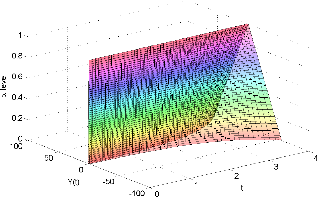
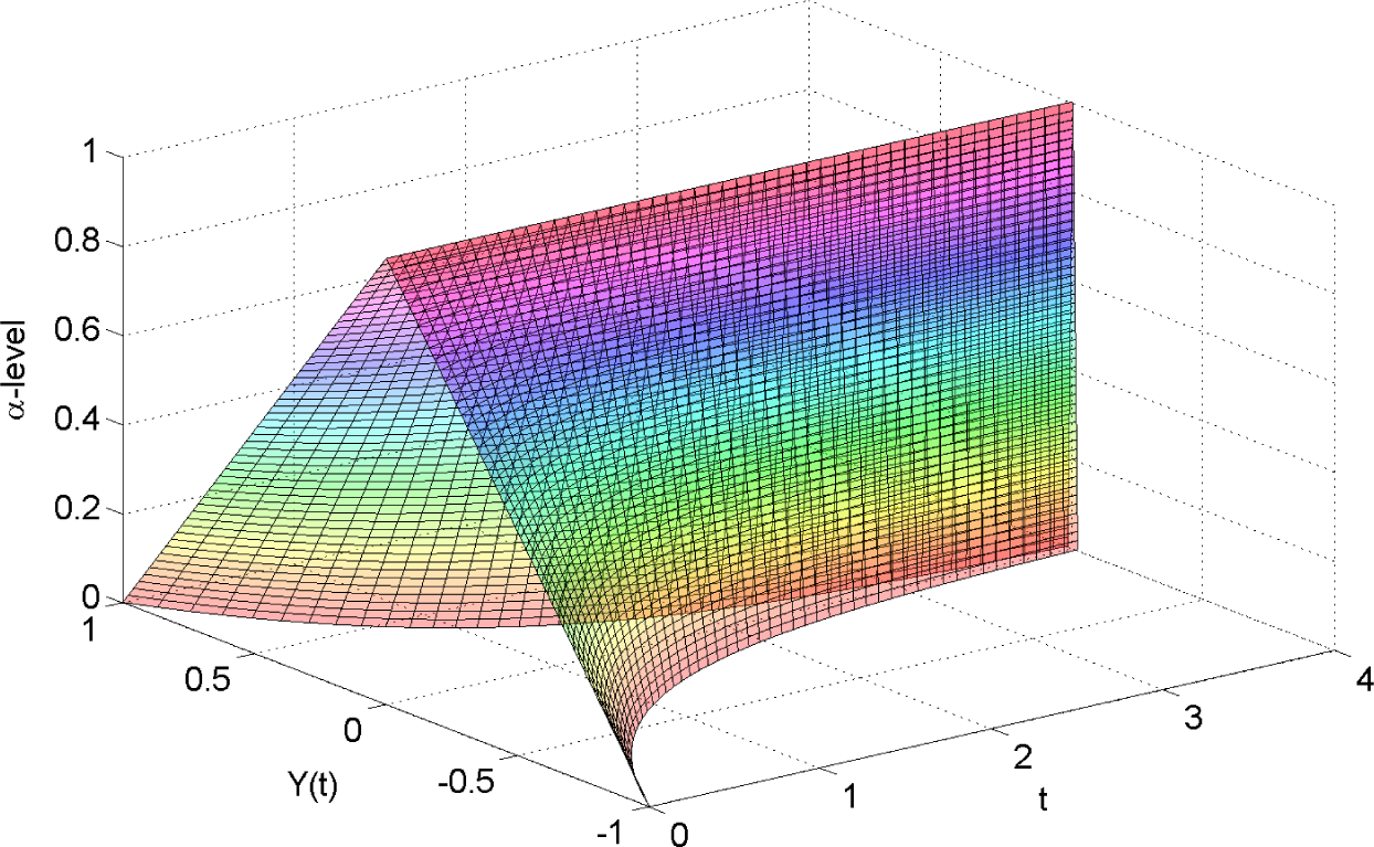
5. A Numerical Example

In this section, we provide a numerical example of solving an FDE using the FST.
Example 1. Consider the following initial value problem:
{ Y ( t ) = Y ( t ) , 0 t T , Y ( t 0 ) = [ y ¯ α ( 0 ) , y ¯ α ( 0 ) ] , 0 < α 1.
By using FST, we have:
S [ Y ( t ) ] = S [ Y ( t ) ]
and:
S [ Y ( t ) ] = 0 Y ( u t ) e t d t .
First, we consider the condition where Y′(t) is (1)-differentiable. Therefore, from Theorem 2,
{ y ¯ α ( t ) = y ¯ α ( t ) , y ¯ α ( t 0 ) = y ¯ α ( 0 ) , y ¯ α ( t ) = y ¯ α ( t ) , y ¯ α ( t 0 ) = y ¯ α ( 0 ) .
By Theorem 7,
S [ Y ( t ) ] = S [ Y ( t ) ] H Y ( t 0 ) u .
Therefore,
S [ Y ( t ) ] = S [ Y ( t ) ] H Y ( t 0 ) u , S [ Y ( t ) ] = S [ Y ( t ) ] H Y ( t 0 ) u .
From Equation (9), we have:
s [ y ¯ α ( t ) ] = s [ y ¯ α ( t ) ] ( y ¯ α ( 0 ) ) u ,
and:
s [ y ¯ α ( t ) ] = s [ y ¯ α ( t ) ] ( y ¯ α ( 0 ) ) u .
Then, we obtain
s [ y ¯ α ( t ) ] = y ¯ α ( 0 ) ( 1 1 u 2 ) y ¯ α ( 0 ) ( u 1 u 2 ) ,
and:
s [ y ¯ α ( t ) ] = y ¯ α ( 0 ) ( 1 1 u 2 ) y ¯ α ( 0 ) ( u 1 u 2 ) .
Thus,
y ¯ α ( t ) = y ¯ α ( 0 ) s 1 ( 1 1 u 2 ) y ¯ α ( 0 ) s 1 ( u 1 u 2 ) ,
and:
y ¯ α ( t ) = y ¯ α ( 0 ) s 1 ( 1 1 u 2 ) y ¯ α ( 0 ) s 1 ( u 1 u 2 ) .
Therefore,
y ¯ α ( t ) = e t ( y ¯ α ( 0 ) y ¯ α ( 0 ) 2 ) + e t ( y ¯ α ( 0 ) + y ¯ α ( 0 ) 2 ) ,
and:
y ¯ α ( t ) = e t ( y ¯ α ( 0 ) y ¯ α ( 0 ) 2 ) + e t ( y ¯ α ( 0 ) + y ¯ α ( 0 ) 2 ) .
Next, we consider the condition where Y′(t) is (2)-differentiable. Therefore, from Theorem 2,
{ y ¯ α ( t ) = y ¯ α ( t ) , y ¯ α ( t 0 ) = y ¯ α ( 0 ) , y ¯ α ( t ) = y ¯ α ( t ) , y ¯ α ( t 0 ) = y ¯ α ( 0 ) .
By Theorem 7,
S [ Y ( t ) ] = ( Y ( t 0 ) ) H ( S [ Y ( t ) ] ) u .
Therefore,
S [ Y ( t ) ] = ( Y ( t 0 ) ) H ( S [ Y ( t ) ] ) u , S [ Y ( t ) ] = ( Y ( t 0 ) ) H ( S [ Y ( t ) ] u .
From Equation (11), we have:
s [ y ¯ α ( t ) ] = s [ y ¯ α ( t ) ] ( y ¯ α ( 0 ) ) u ,
and:
s [ y ¯ α ( t ) ] = s [ y ¯ α ( t ) ] ( y ¯ α ( 0 ) ) u .
Then, we obtain:
s [ y ¯ α ( t ) ] = y ¯ α ( 0 ) ( 1 1 + u ) ,
and:
s [ y ¯ α ( t ) ] = y ¯ α ( 0 ) ( u 1 + u ) .
Therefore,
y ¯ α ( t ) = y ¯ α ( 0 ) e 1 ,
and:
y ¯ α ( t ) = y ¯ α ( 0 ) e 1 .
Assume that [ y ¯ α ( t 0 ) , y ¯ α ( t 0 ) ] = [ α a , a α ]. Then, the solutions of Equation (12) for Case (1) and Case (2) are as follows.
Case 1:
y ¯ α ( t ) = ( α a ) e t , y ¯ α ( t ) = ( a α ) e t .
Case 2:
y ¯ α ( t ) = ( α a ) e t , y ¯ α ( t ) = ( a α ) e t .
The results obtained using the FST for both cases proposed in this paper are shown in Figures 1 and 2, respectively. We can see that for Case 1, the result diverges as t increases; while for Case 2, the result implicates that the solution converges as t increases.
Remark. From the example, we notice that the solutions depend on the differential equation we chose. For Case 1, the solution has the property that the diameter, i.e. diam(supp y(t)) = 2aet, which is unbounded as t approaches infinity. Comparing to Case 2, the diam(supp y(t)) = 2ae−t 0 as t approaches infinity, which leads to much more intuitive results.

6. Conclusions

In this paper, we have studied the classical Sumudu transform in the fuzzy setting. We have also proposed detailed procedures to solve FDEs. In the last part, we have conducted a numerical example of solving first order linear FDE using the FST.

Acknowledgments

This research was supported by the Fundamental Research Grant Scheme of Ministry of Science, Technology and Innovation, Malaysia, under Project Code 9003-00417.

Author Contributions

Both authors have read and agreed on the submission of this paper. Furthermore, both authors have contributed to every part of this paper. Both authors have read and approved the final manuscript.

Conflicts of Interest

The authors declare no conflict of interest.

References

  1. Davis, J.A.; McNamara, D.E.; Cottrell, D.M.; Campos, J. Image processing with the radial Hilbert transform: Theory and experiments. Opt. Lett. 2000, 25, 99–101. [Google Scholar]
  2. Namias, V. The fractional order Fourier transform and its application to quantum mechanics. IMA J. Appl. Math. 1980, 25, 241–265. [Google Scholar]
  3. Saitoh, S. The Weierstrass transform and an isometry in the heat equation. Appl. Anal. 1983, 16, 1–6. [Google Scholar]
  4. Ghaemi, F.; Yunus, R.; Ahmadian, A.; Salahshour, S.; Suleiman, M.; Saleh, S.F. Application of Fuzzy Fractional Kinetic Equations to Modelling of the Acid Hydrolysis Reaction. Abstr. Appl. Anal. 2013, 2013, 610314. [Google Scholar]
  5. Spinelli, R. Numerical inversion of a Laplace transform. SIAM J. Numer. Anal. 1966, 3, 636–649. [Google Scholar]
  6. Layman, J.W. The Hankel transform and some of its properties. J. Integer Seq. 2001, 4, 1–11. [Google Scholar]
  7. Tranter, C. The use of the Mellin transform in finding the stress distribution in an infinite wedge. Q. J. Mech. Appl. Math. 1948, 1, 125–130. [Google Scholar]
  8. Watugala, G.K. Sumudu transforms—A new integral transform to solve differential equations and control engineering problems. Int. J. Math. Educ. Sci. Technol. 1993, 24, 35–43. [Google Scholar]
  9. Watugala, G.K. Sumudu transforms-a new integral transform to solve differential equations and control engineering problems. Math. Eng. Ind. 1998, 6, 319–329. [Google Scholar]
  10. Weerakoon, S. Application of Sumudu transform to partial differential equations. Int. J. Math. Educ. Sci. Technol. 1994, 25, 277–283. [Google Scholar]
  11. Weerakoon, S. Complex inversion formula for Sumudu transform. Int. J. Math. Educ. Sci. Technol. 1998, 29, 618–621. [Google Scholar]
  12. Asiru, M.A. Sumudu transform and the solution of integral equations of convolution type. Int. J. Math. Educ. Sci. Technol. 2001, 32, 906–910. [Google Scholar]
  13. Belgacem, F.B.M.; Karaballi, A.A.; Kalla, S.L. Analytical investigations of the Sumudu transform and applications to integral production equations. Math. Probl. Eng. 2003, 2003, 103–118. [Google Scholar]
  14. Belgacem, F.B.M.; Karaballi, A.A. Sumudu transform fundamental properties investigations and applications. Int. J. Stoch. Anal. 2006, 2006. [Google Scholar] [CrossRef]
  15. Belgacem, F.B.M. Sumudu transform applications to Bessel functions and equations. Appl. Math. Sci. 2010, 4, 3665–3686. [Google Scholar]
  16. Agwa, H.A.; Ali, F.M.; Kılıçman, A. A new integral transform on time scales and its application. Adv. Differ. Equ. 2012, 2012. [Google Scholar] [CrossRef]
  17. Kılıçman, A.; Eltayeb, H.; Ismail, M.R. A note on integral transforms and differential equations. Malays. J. Math. Sci. 2012, 6, 1–18. [Google Scholar]
  18. Asiru, M.A. Further properties of the Sumudu transform and its application. Int. J. Math. Educ. Sci. Technol. 2002, 33, 441–449. [Google Scholar]
  19. Eltayeb, H.; Kılıçman, A. A note on the Sumudu transforms and differential equations. Appl. Math. Sci. 2010, 4, 1089–1098. [Google Scholar]
  20. Belgacem, F.B.M. Introducing and analyzing deeper Sumudu properties. Nonlinear Stud. 2006, 13, 23–41. [Google Scholar]
  21. Rathore, S.; Kumar, D.; Singh, J.; Gupta, S. Homotopy analysis Sumudu transform method for nonlinear equations. Int. J. Ind. Math. 2012, 4, 301–314. [Google Scholar]
  22. Zadeh, L.A. Fuzzy sets. Inf. Control. 1965, 8, 338–353. [Google Scholar]
  23. Chang, S.S.L.; Zadeh, L.A. On fuzzy mapping and control. IEEE Trans. Syst. Man Cybern. 1972, SMC-2, 30–34. [Google Scholar]
  24. Dubois, D.; Prade, H. Towards fuzzy differential calculus part 1: Integration of fuzzy mappings. Fuzzy Sets Syst. 1982, 8, 1–17. [Google Scholar]
  25. Dubois, D.; Prade, H. Towards fuzzy differential calculus part 2: Integration on fuzzy intervals. Fuzzy Sets Syst. 1982, 8, 105–116. [Google Scholar]
  26. Dubois, D.; Prade, H. Towards fuzzy differential calculus part 3: Differentiation. Fuzzy Sets Syst. 1982, 8, 225–233. [Google Scholar]
  27. Puri, M.L.; Ralescu, D.A. Differentials of fuzzy functions. J. Math. Anal. Appl. 1983, 91, 552–558. [Google Scholar]
  28. Goetschel, R., Jr.; Voxman, W. Elementary fuzzy calculus. Fuzzy Sets Syst. 1986, 18, 31–43. [Google Scholar]
  29. Kaleva, O. Fuzzy differential equations. Fuzzy Sets Syst. 1987, 24, 301–317. [Google Scholar]
  30. Ding, Z.; Ma, M.; Kandel, A. Existence of the solutions of fuzzy differential equations with parameters. Inf. Sci. 1997, 99, 205–217. [Google Scholar]
  31. Salahshour, S. Nth-order fuzzy differential equations under generalized differentiability. J. Fuzzy Set Valued Anal. 2011, 2011. [Google Scholar] [CrossRef]
  32. Shahriyar, M.; Ismail, F.; Aghabeigi, S.; Ahmadian, A.; Salahshour, S. An eigenvalue-eigenvector method for solving a system of fractional differential equations with uncertainty. Math. Probl. Eng. 2013, 2013, 579761. [Google Scholar]
  33. Arshad, S.; Lupulescu, V. On the fractional differential equations with uncertainty. Nonlinear Anal. Theory Methods Appl. 2011, 74, 3685–3693. [Google Scholar]
  34. Allahviranloo, T.; Salahshour, S.; Abbasbandy, S. Explicit solutions of fractional differential equations with uncertainty. Soft Comput. 2012, 16, 297–302. [Google Scholar]
  35. Allahviranloo, T.; Ahmadi, M.B. Fuzzy Laplace transforms. Soft Comput. 2010, 14, 235–243. [Google Scholar]
  36. Salahshour, S.; Allahviranloo, T. Applications of fuzzy Laplace transforms. Soft Comput. 2013, 17, 145–158. [Google Scholar]
  37. Jafarian, A.; Golmankhaneh, A.K.; Baleanu, D. On fuzzy fractional Laplace transformation. Adv. Math. Phys. 2014, 2014. [Google Scholar] [CrossRef]
  38. Salahshour, S.; Allahviranloo, T.; Abbasbandy, S. Solving fuzzy fractional differential equations by fuzzy Laplace transforms. Commun. Nonlinear Sci. Numer. Simul. 2012, 17, 1372–1381. [Google Scholar]
  39. Salahshour, S.; Khezerloo, M.; Hajighasemi, S.; Khorasany, M. Solving fuzzy integral equations of the second kind by fuzzy Laplace transform method. Int. J. Ind. Math. 2012, 4, 21–29. [Google Scholar]
  40. Muhammad Ali, H.F.; Haydar, A.K. On fuzzy Laplace transforms for fuzzy differential equations of the third order. J. Kerbala Univ. 2013, 11, 251–256. [Google Scholar]
  41. Salahshour, S.; Haghi, E. Solving fuzzy heat equation by fuzzy Laplace transforms, Information Processing and Management of Uncertainty in Knowledge-Based Systems; Springer: Berlin/Heidelberg, Germany, 2010; pp. 512–521.
  42. Ahmad, M.Z.; Abdul Rahman, N.A. Explicit solution of fuzzy differential equations by mean of fuzzy Sumudu transform. Int. J. Appl. Phys. Math. 2015, 5, 86–93. [Google Scholar]
  43. Alam Khan, N.; Abdul Razzaq, O.; Ayyaz, M. On the solution of fuzzy differential equations by fuzzy Sumudu transform. Nonlinear Eng. 2015, 4, 49–60. [Google Scholar]
  44. Xu, J.; Liao, Z.; Hu, Z. A class of linear differential dynamical systems with fuzzy initial condition. Fuzzy Sets Syst. 2007, 158, 2339–2358. [Google Scholar]
  45. Zimmerman, H.J. Fuzzy Set Theory and Its Applications; Kluwer Academic Publisher and Dordrecht: Dordrecht, The Netherlands, 1991. [Google Scholar]
  46. Friedman, M.; Ma, M.; Kandel, A. Numerical solutions of fuzzy differential and integral equations. Fuzzy Sets Syst. 1999, 106, 35–48. [Google Scholar]
  47. Ma, M.; Friedman, M.; Kandel, A. Numerical solutions of fuzzy differential equations. Fuzzy Sets Syst. 1999, 105, 133–138. [Google Scholar]
  48. Ahmad, M.Z.; de Baets, B. A Predator-Prey Model with Fuzzy Initial Populations. Proceedings of the Joint 2009 International Fuzzy Systems Association World Congress and 2009 European Society of Fuzzy Logic and Technology Conference, Lisbon, Portugal, 20–24 July 2009; pp. 1311–1314.
  49. Dubois, D.J. Fuzzy Sets and Systems: Theory and Applications; Academic Press: Waltham, MA, USA, 1980. [Google Scholar]
  50. Wu, H.C. The improper fuzzy Riemann integral and its numerical integration. Inf. Sci. 1998, 111, 109–137. [Google Scholar]
  51. Wu, H.C. The fuzzy Riemann integral and its numerical integration. Fuzzy Sets Syst. 2000, 110, 1–25. [Google Scholar]
  52. Bede, B.; Gal, S.G. Generalizations of the differentiability of fuzzy-number-valued functions with applications to fuzzy differential equations. Fuzzy Sets Syst. 2005, 151, 581–599. [Google Scholar]
  53. Bede, B.; Rudas, I.J.; Bencsik, A.L. First order linear fuzzy differential equations under generalized differentiability. Inf. Sci. 2007, 177, 1648–1662. [Google Scholar]
  54. Chalco-Cano, Y.; Román-Flores, H. On new solutions of fuzzy differential equations. Chaos Solitons Fractals. 2008, 38, 112–119. [Google Scholar]
  55. Das, M.; Talukdar, D. Method For Solving Fuzzy Integro-Differential Equation By Using Fuzzy Laplace Transformation. Int. J. Sci. Technol. Res. 2014, 3, 291–295. [Google Scholar]
  56. Chalco-Cano, Y.; Román-Flores, H. Comparation between some approaches to solve fuzzy differential equations. Fuzzy Sets Syst. 2009, 160, 1517–1527. [Google Scholar]
  57. Kaleva, O. A note on fuzzy differential equations. Nonlinear Anal. Theory Methods Appl. 2006, 64, 895–900. [Google Scholar]
Figure 1. The solution of Equation (12) for Case 1 when Y(t0) = (1, 0, 1).
Entropy 17 04582f1
Figure 2. The solution of Equation (12) for Case 2 when Y(t0) = (1, 0, 1).
Entropy 17 04582f2

