Secrecy Capacity of the Extended Wiretap Channel II with Noise

Abstract

The secrecy capacity of an extended communication model of wiretap channelII is determined. In this channel model, the source message is encoded into a digital sequence of length N and transmitted to the legitimate receiver through a discrete memoryless channel (DMC). There exists an eavesdropper who is able to observe arbitrary $\mu =N\alpha$ digital symbols from the transmitter through a second DMC, where $0\le \alpha \le 1$ is a constant real number. A pair of an encoder and a decoder is designed to let the receiver be able to recover the source message with a vanishing decoding error probability and keep the eavesdropper ignorant of the message. This communication model includes a variety of wiretap channels as special cases. The coding scheme is based on that designed by Ozarow and Wyner for the classic wiretap channel II.

1. Introduction

The concept of the wiretap channel was first introduced by Wyner. In his celebrated paper [1], Wyner considered a communication model, where the transmitter communicated with the legitimate receiver through a discrete memoryless channel (DMC). Meanwhile, there existed an eavesdropper observing the digital sequence from the receiver through a second DMC. The goal was to design a pair of an encoder and a decoder such that the receiver was able to recover the source message perfectly, while the eavesdropper was ignorant of the message. That communication model is actually a degraded discrete memoryless wiretap channel.

After that, the communication models of wiretap channels have been studied from various aspects. Csiszár and Körner [2] considered a more general wiretap channel where the wiretap channel did not need to be a degraded version of the main channel, and common messages were also considered there. Other communication models of wiretap channels include wiretap channels with side information [3,4,5,6,7,8], compound wiretap channels [9,10,11,12] and arbitrarily-varying wiretap channels [13].

Ozarow and Wyner studied another kind of wiretap channel called the wiretap channel II [14]. The source message W was encoded into digital bits $X^N$ and transmitted to the legitimate receiver via a binary noiseless channel. An eavesdropper could observe arbitrary $\mu =N\alpha$ digital bits from the receiver, where $0<\alpha <1$ is a constant real number not dependent on N.

Some extensions of the wiretap channel have been studied in recent years.

Cai and Yeung extended the wiretap channel II into the network scenario [15,16]. In that network model, the source message of length K was transmitted to the legitimate users through a network, and the eavesdropper was able to wiretap on at most $\mu <K$ edges. Cai and Yeung suggested using a linear “secret-sharing” method to provide security in the network. Instead of sending K message symbols, the source node sent μ random symbols and $K-\mu$ message symbols. Additionally, the code itself underwent a certain linear transformation. Cai and Yeung gave sufficient conditions for this transformation to guarantee security. They showed that as long as the field size is sufficiently large, a secure transformation existed. Some related work on wiretap networks was given in [17,18,19,20].

An extension of wiretap channel II was considered recently in [21,22]. The source message was encoded into the digital sequence $X^N$ and transmitted to the legitimate receiver via a DMC. The eavesdropper could observe any $\mu =N\alpha$ digital bits of $X^N$ from the transmitter. A pair of inner-outer bounds was given in [21], while the secrecy capacity with respect to the semantic secrecy criterion was established in [22]. The coding scheme in [21] was based on that developed by Ozarow and Wyner in [14], while the scheme in [22] was by Wyner’s soft covering lemma. He et al. considered another extension of wiretap channel II in [23]. In that model, the eavesdropper observed arbitrary $\mu =N\alpha$ digital bits of the main channel output $Y^N$ from the receiver. The capacity with respect to the strong secrecy criterion was established there. The proof of the coding theorem was based on Csiszár’s almost independent coloring scheme. Some other work on wiretap channel II can be found in [24,25,26].

This paper considers a more general extension of wiretap channel II, where the eavesdropper observes arbitrary μ digital bits from the transmitter via a second DMC. The capacity with respect to the weak secrecy criteria is established. The coding scheme is based on that developed by Ozarow and Wyner in [14]. It is obvious that this communication model includes the general discrete memoryless wiretap channels, the wiretap channel II and the communication models discussed in [21,22,23] as special cases. Nevertheless, we should notice that the secrecy criteria considered in [22,23] are strictly stronger than those considered in this paper; see Figure 1.

The remainder of this paper is organized as follows. The formal statement and the main results are given in Section 2. The secrecy capacity is formulated in Theorem 1, whose proof is discussed in Section 4. Section 5 provides a binary example of this model. Section 6 gives a final conclusion of this paper.

2. Notation and Problem Statements

Throughout the paper, $\mathbb{N}$ is the set of positive integers and $[1:N]=\{1,2,\dots ,N\}$ for any $N\in \mathbb{N}$. ${\mathfrak{I}}_{\mu }={\mathfrak{I}}_{\mu }\left(N\right)=\{\mathcal{I}\subseteq [1:N]:|\mathcal{I}|=\mu \}$ represents the collection of subsets of $[1:N]$ with size μ.

Random variables, sample values and alphabets (sets) are denoted by capital letters, lower case letters and calligraphic letters, respectively. A similar convention is applied to random vectors and their sample values. For example, $X^N$ represents a random N-vector ($X_1,X_2,\dots ,X_N$), and $x^N$ is a specific vector of $X^N$ in ${\mathcal{X}}^N$. ${\mathcal{X}}^N$ is the N-th Cartesian power of $\mathcal{X}$.

Let ‘?’ be a “dummy” letter. For any index set $\mathcal{I}\subseteq [1:N]$ and finite alphabet $\mathcal{X}$ not containing the “dummy” letter ‘?’, denote:

$${\mathcal{X}}_{\mathcal{I}}^N=\{(x_1,x_2,\dots ,x_N):x_i\in \mathcal{X}\mathrm{if}i\in \mathcal{I},\mathrm{and}{x}_i=?\mathrm{otherwise}\}.$$

For any given random vector $X^N=(X_1,X_2,\dots ,X_N)$ and index set $\mathcal{I}\subseteq [1:N]$,

• $X_{\mathcal{I}}^N=(X_1^{\prime },X_2^{\prime },\dots ,X_N^{\prime })$ is a “projection” of $X^N$ onto $\mathcal{I}$ with $X_n^{\prime }=X_n$ for $n\in \mathcal{I}$, and $X_n^{\prime }=?$ otherwise.
• $X_{\mathcal{I}}=(X_i,i\in \mathcal{I})$ is a subvector of $X^N$.

The random vector $X_{\mathcal{I}}^N$ takes the value from ${\mathcal{X}}_{\mathcal{I}}^N$, while the random vector $X_{\mathcal{I}}$ takes the value from ${\mathcal{X}}^{\left|\mathcal{I}\right|}$.

Example 1.

Supposing that $N=5$, the index set $\mathcal{I}=\{1,3,5\}$ and the random vector $X^N=(X_1,X_2,X_3,X_4,X_5)$, we have $X_{\mathcal{I}}^N=(X_1,?,X_3,?,X_5)$ and $X_{\mathcal{I}}=(X_1,X_3,X_5)$.

The communication model in this paper, which is shown in Figure 2, is composed of an encoder, the main channel, the wiretap channel and a decoder. The definitions of these parts are from Definition 1 to Definition 4, respectively. The definition of achievability is in Definition 5.

Definition 1.

(Encoder) The source message W is uniformly distributed on the message set $\mathcal{W}=[1:M]$. The (stochastic) encoder is specified by a matrix of conditional probability $En\left(x^N\right|w)$ for the channel input $x^N\in {\mathcal{X}}^N$ and message $w\in \mathcal{W}$.

Definition 2.

(Main channel) The main channel is a DMC with finite input alphabet $\mathcal{X}$ and finite output alphabet $\mathcal{Y}$, where $?\notin \mathcal{X}\cup \mathcal{Y}$. The transition probability is $Q_M\left(y\right|x)$. Let $X^N$ and $Y^N$ denote the input and output of the main channel, respectively. It follows that for any $x^N\in {\mathcal{X}}^N$ and $y^N\in {\mathcal{Y}}^N$,

$$\mathrm{Pr}\{X^N=x^N,Y^N=y^N\}=\mathrm{Pr}\{X^N=x^N\}{Q}_M^N\left(y^N\right|x^N)$$

where:

$$Q_M^N\left(y^N\right|x^N)=\prod _{n=1}^N{Q}_M\left(y_n\right|x_n).$$

Definition 3.

(Wiretap channel) The eavesdropper is able to observe arbitrary $\mu =N\alpha$ digital bits from the transmitter via another DMC, whose transition probability is denoted as $Q_W\left(z\right|x)$ with $x\in \mathcal{X}$ and $z\in \mathcal{Z}$. The alphabet $\mathcal{Z}$ does not contain the “dummy” letter ‘?’ either. The input $X^N$ and the output $Z^N$ of the wiretap channel satisfy that:

$$\mathrm{Pr}\{X^N=x^N,Z^N=z^N\}=\mathrm{Pr}\{X^N=x^N\}{Q}_W^N\left(z^N\right|x^N)$$

with:

$$Q_W^N\left(z^N\right|x^N)=\prod _{n=1}^N{Q}_W\left(z_n\right|x_n).$$

Supposing that the eavesdropper observes digital bits of the wiretap channel output $Z^N$ whose indices lie in the observing index set $\mathcal{I}$, the subsequence obtained by the eavesdropper can then be denoted by ${\tilde{Z}}^N=Z_{\mathcal{I}}^N$. Therefore, the information on the source message (of each bit) exposed to the eavesdropper is denoted by:

$$\mathrm{\Delta }=\underset{\mathcal{I}\in {\mathfrak{I}}_{\mu }}{\max }\frac{1}{N}I(W;Z_{\mathcal{I}}^N).$$

Remark 1.

Clearly, for given wiretap channel output ${\tilde{Z}}^N$, one can easily determine which subsequence of $Z^N$ is observed by the eavesdropper. More precisely, ${\tilde{Z}}^N=Z_{\mathcal{I}}^N$ with $\mathcal{I}=\mathcal{I}({\tilde{Z}}^N)=\{i:{\tilde{Z}}_i\ne ?\}$.

Definition 4.

(Decoder) The decoder is a mapping $\varphi :{\mathcal{Y}}^N\mapsto \mathcal{W}$, with $Y^N$ as the input and $\widehat{W}=\varphi \left(Y^N\right)$ as the output. The average decoding error probability is defined as $P_e=\mathrm{Pr}\{W\ne \widehat{W}\}.$

Definition 5.

(Achievability) A non-negative real number R is said to be achievable, if for any $ϵ>0$, there exists an integer $N_0$, such that one can construct an $(N,M)$ code satisfying:

$$\frac{1}{N}\log M\ge R-ϵ,$$

(1)

$$P_e\le ϵ$$

(2)

and:

$$\mathrm{\Delta }<ϵ,$$

(3)

where $N>N_0$. The capacity, or the maximal achievable transmission rate, of the communication model is denoted by $C_s$.

Remark 2.

Notice that the capacities defined in this paper are under the condition of negligible average decoding error probability, but one can construct the coding schemes for the negligible maximal decoding error probability through the standard techniques. See Appendix A for details.

3. Main Result

Theorem 1.

The capacity of the communication model described in Figure 2 is:

$$C_s=\underset{P_U·P_{X|U}:U\to X\to YZ}{\max }[I(U;Y)-\alpha I(U;Z)],$$

where U is an auxiliary random variable distributed on $\mathcal{U}$ with $\left|\mathcal{U}\right|\le \left|\mathcal{X}\right|$.

The converse half of Theorem 1 can be established quite similarly to the method of establishing the converse of Theorem 2 in [22], and hence, we omit it here. The direct part of Theorem 1 is given in Section 4.

Corollary 1.

When $\alpha =1$, the communication model is transformed into a general discrete memoryless wiretap channel, whose capacity is formulated by:

$$C_s=\underset{P_U·P_{X|U}:U\to X\to YZ}{\max }[I(U;Y)-I(U;Z)].$$

The result coincides with that of Corollary 2 in [2]. In particular, if $X\to Y\to Z$ forms a Markov chain, the capacity is further deduced by:

$$\begin{array}{cc}\hfill C_s& {\displaystyle =\underset{P_U·P_{X|U}:U\to X\to Y\to Z}{\max }[I(U;Y)-I(U;Z)]}\hfill \\ & \stackrel{\left(a\right)}{=}{\displaystyle \underset{P_U·P_{X|U}:U\to X\to Y\to Z}{\max }\left[I(U;Y|Z)\right]}\hfill \\ & \stackrel{\left(b\right)}{=}{\displaystyle \underset{P_X:X\to Y\to Z}{\max }\left[I(X;Y|Z)\right]}\hfill \\ & \stackrel{\left(c\right)}{=}{\displaystyle \underset{P_X:X\to Y\to Z}{\max }[I(X;Y)-I(X;Z)],}\hfill \end{array}$$

where (a) follows because $U\to Y\to Z$ forms a Markov chain, (b) follows because the Markov chain $U\to X\to Y$ for a given Z implies that $I(U;Y|Z)\le I(X;Y\left|Z\right)$ and the equality holds if and only if $U=X$ and (c) follows because $X\to Y\to Z$ forms a Markov chain.

Corollary 2.

When $Y=Z$, i.e., the eavesdropper observes $\mu =N\alpha$ digital bits from the receiver, the communication model is transformed into that studied in [23]. In this case, the capacity is formulated by:

$$C_s=\underset{P_U·P_{X|U}:U\to X\to Y}{\max }(1-\alpha )I(U;Y)=\underset{P_X}{\max }(1-\alpha )I(X;Y),$$

where the last equality follows because the Markov chain $U\to X\to Y$ implies that $I(U;Y)\le I(X;Y)$ and the equality holds if and only if $U=X$.

Notice that [23] considered the capacity with respect to the strong secrecy criterion, while the current paper considers that with the weak secrecy criterion. Therefore, Theorem 1 in [23] and Corollary 2 in the current paper indicate that the capacity with respect to the strong secrecy criterion is identical to that with the weak secrecy criterion.

Corollary 3.

When $Z=X$, i.e., the eavesdropper observes $\mu =N\alpha$ digital bits from the transmitter, the communication model is transformed into that studied in [21,22]. In this case, the capacity is formulated by:

$$C_s=\underset{P_U·P_{X|U}:U\to X\to Y}{\max }[I(U;Y)-\alpha I(U;X)].$$

The channel model described in Corollary 3 was first studied in [21], and a pair of inner and outer bounds was given there. The secrecy capacity with respect to the semantic secrecy criterion, which is identical to the capacity with the weak criterion given in Corollary 3, was established in [22].

4. Direct Part of Theorem 1

This section proves the direct part of Theorem 1. Let an arbitrary quadruple of random variables $(U^{*},X^{*},Y^{*},Z^{*})$ be given, which satisfy that:

$$\mathrm{Pr}\{U^{*}=u,X^{*}=x,Y^{*}=y,Z^{*}=z\}=P_{U^{*}}\left(u\right)P_{X^{*}|U^{*}}\left(x\right|u)Q_M\left(y\right|x)Q_W\left(z\right|x)$$

(4)

for $(u,x,y,z)\in \mathcal{U}\times \mathcal{X}\times \mathcal{Y}\times \mathcal{Z}$. The goal of this section is to establish that every real number R satisfying $0\le R<I(U^{*};Y^{*})-\alpha I(U^{*};Z^{*})$ is achievable. In fact, it suffices to prove the achievability of every R satisfying:

$$0\le R<I(X^{*};Y^{*})-\alpha I(X^{*};Z^{*}).$$

(5)

To show this, suppose that every transmission rate R satisfying Equation (5) is achievable. For any random variable $U^{*}$ satisfying Equation (4), the encoder could deliberately increase the noise of the communication system by inserting a virtual noisy channel $Q_V$ at the transmitting port of the system, such that:

$$Q_V\left(x\right|u)=P_{X^{*}|U^{*}}\left(x\right|u).$$

This would create the virtual communication system depicted in Figure 3, where the transition matrix of the main channel is:

$${\tilde{Q}}_M\left(y\right|u)=P_{Y^{*}|U^{*}}\left(y\right|u)=\sum _{x\in \mathcal{X}}{Q}_V\left(x\right|u)Q_M\left(y\right|x)$$

and the transition matrix of the wiretap channel is:

$${\tilde{Q}}_W\left(z\right|u)=P_{Z^{*}|U^{*}}\left(y\right|u)=\sum _{x\in \mathcal{X}}{Q}_V\left(x\right|u)Q_W\left(y\right|x).$$

It is clear that every real number $0<R\le I(U^{*};Y^{*})-\alpha I(U^{*};Z^{*})$ is achievable for the virtual system and hence is achievable for the original system.

In the remainder of this section, it will be shown that every transmission rate R satisfying Equation (5) is achievable. To be precise, for any ϵ and τ satisfying $0<ϵ\le \tau <I(X^{*};Y^{*})-\alpha I(X^{*};Z^{*})$, we need to establish that there exists an $(N,M)$ code, such that:

$$\frac{1}{N}\log M\ge I(X^{*};Y^{*})-\alpha I(X^{*};Z^{*})-\tau >0,$$

(6)

$$\mathrm{\Delta }=\underset{\mathcal{I}\in {\mathfrak{I}}_{\mu }}{\max }\frac{1}{N}I(W;Z_{\mathcal{I}}^N)<ϵ,$$

(7)

and:

$$P_e<ϵ$$

(8)

when N is sufficiently large.

The coding scheme is based on the scheme developed by Ozarow and Wyner [14] for the classic wiretap channel II. In that channel model, for each wiretap channel output $z^N$, there exists a collection of codewords that are “consistent” with it, namely the codewords that could produce the wiretap channel output $z^N$ for some observing index $\mathcal{I}$. Ozarow and Wyner constructed a secure partition, such that the number of “consistent” codewords, for every wiretap channel output $z^N$, in each sub-code is less than a constant integer. However, it is not feasible to consider the “consistent” codewords in our model, where the wiretap channel may be noisy. Instead, we construct a secure partition such that the number of codewords, jointly typical with the wiretap channel output $z^N$, in each sub-code is less than a constant integer.

The proof is organized as follows. Firstly, Section 4.1 gives some definitions on the typicality of μ-subsequences and lists some basic results. Then, the construction of the encoder and decoder is introduced in Section 4.2. The key point is to generate a “good” codebook with the desired partition to ensure secrecy. Thirdly, as the main part of the proof, Section 4.3 shows the existence of a “good” codebook with the desired partition. For any $ϵ>0$ and $\tau >0$, the proof that the coding scheme in Section 4.2 satisfies the requirements of the transmission rate, reliability and security, namely Formulas (6) to (8), is finally detailed in Section 4.4.

4.1. Typicality

The definitions of letter typicality on a given index set follow from those briefly introduced in [23]. We list them in this subsection for the sake of completeness.

Firstly, the original definitions of letter typicality are given as follows. Please refer to Chapter 1 in [27] for more details.

For any $\delta \ge 0$, the δ-letter typical set $T_{\delta }^N\left(P_X\right)$ with respect to the probability distribution $P_X$ on $\mathcal{X}$ is the set of $x^N\in {\mathcal{X}}^N$ satisfying:

$$|\frac{1}{N}\mathbf{N}\left(a\right|x^N)-P_X\left(a\right)|\le \delta P_X\left(a\right)\mathrm{for}\mathrm{all}a\in \mathcal{X},$$

where $\mathbf{N}\left(a\right|x^N)$ is the number of positions of $x^N$ having the letter $a\in \mathcal{X}$.

Similarly, let $\mathbf{N}(a,b|x^N,y^N)$ be the number of times that the pair $(a,b)$ occurs in the sequence of pairs $(x_1,y_1),(x_2,y_2),\dots ,(x_N,y_N)$. The jointly typical set $T_{\delta }^N\left(P_{XY}\right)$, with respect to the joint probability distribution $P_{XY}$ on $\mathcal{X}\times \mathcal{Y}$, is the set of sequence pairs $(x^N,y^N)\in {\mathcal{X}}^N\times {\mathcal{Y}}^N$ satisfying:

$$|\frac{1}{N}\mathbf{N}(a,b|x^N,y^N)-P_{XY}(a,b)|\le \delta P_{XY}(a,b)$$

for all $(a,b)\in \mathcal{X}\times \mathcal{Y}.$

For any given $x^N\in {\mathcal{X}}^N$, the conditionally typical set of $x^N$ with respect to the joint mass function $P_{XY}$ is defined as:

$$T_{\delta }^N\left(P_{XY}\right|x^N)=\{y^N\in {\mathcal{Y}}^N:(x^N,y^N)\in T_{\delta }^N\left(P_{XY}\right)\}.$$

The definitions on the typicality of μ-subsequences on index set $\mathcal{I}\in {\mathfrak{I}}_{\mu }$ and some basic results are given as follows.

Definition 6.

Given a random variable X on $\mathcal{X}$, the letter typical set ${\tilde{T}}_{\mathcal{I}}^N{\left[X\right]}_{\delta }$ with respect to X on the index set $\mathcal{I}\in {\mathfrak{I}}_{\mu }$ is the set of $x^N\in {\mathcal{X}}_{\mathcal{I}}^N$ such that $x_{\mathcal{I}}\in T_{\delta }^{\mu }\left(P_X\right)$, where $x_{\mathcal{I}}$ is the μ-subvector of $x^N$ and $P_X$ is the probability mass function of the random variable X.

Example 2.

Let X be a random variable on the binary set $\mathcal{X}=\{0,1\}$, such that $P_X\left(0\right)=1-P_X\left(1\right)=\frac{1}{5}$. Set $N=10$, $\delta =0.1$ and $\mathcal{I}=[1:5]$. Then:

• the sequence $x^N=0111100000$ is out of $T_{\delta }^N\left(P_X\right)$ while $x_{\mathcal{I}}^N=01111?????$ belongs to ${\tilde{T}}_{\mathcal{I}}^N{\left[X\right]}_{\delta }$;
• the sequence $x^{\prime N}=1111101110$ belongs to $T_{\delta }^N\left(P_X\right)$ while $x_{\mathcal{I}}^{\prime N}=11111?????$ is out of ${\tilde{T}}_{\mathcal{I}}^N{\left[X\right]}_{\delta }$;
• the sequence $x^{″N}=0111111110$ belongs to $T_{\delta }^N\left(P_X\right)$, and $x_{\mathcal{I}}^{″N}=01111?????$ belongs to ${\tilde{T}}_{\mathcal{I}}^N{\left[X\right]}_{\delta }$.

Remark 3.

(Theorem 1.1 in [27]) Suppose that $X_1,X_2,\dots ,X_N$ are N i.i.d. random variables with the same generic probability distribution as that of X. For any given $\mathcal{I}\in {\mathfrak{I}}_{\mu }$ and $\delta <m_X$,

1.

if $x^N\in {\tilde{T}}_{\mathcal{I}}^N{\left[X\right]}_{\delta }$, then

$$2^{-\mu (1+\delta )H\left(X\right)}\le \mathrm{Pr}\{X_{\mathcal{I}}^N=x^N\}\le 2^{-\mu (1-\delta )H\left(X\right)},$$

2.

$\mathrm{Pr}\{X_{\mathcal{I}}^N\in {\tilde{T}}_{\mathcal{I}}^N{\left[X\right]}_{\delta }\}>1-{\widetilde{ϵ}}_1$,

where:

$${\widetilde{ϵ}}_1={\widetilde{ϵ}}_1(\mu ,\delta ,m_X)=2\left|\mathcal{X}\right|e^{-\mu {\delta }^2{m}_X}$$

and $m_X={\min }_{x\in \mathcal{X}:P_X\left(x\right)>0}{P}_X\left(x\right)$.

Definition 7.

Let $(X,Y)$ be a pair of random variables with the joint probability mass function $P_{XY}$ on $\mathcal{X}\times \mathcal{Y}$. The jointly typical set ${\tilde{T}}_{\mathcal{I}}^N{\left[XY\right]}_{\delta }$ with respect to $(X,Y)$ on the index set $\mathcal{I}\in {\mathfrak{I}}_{\mu }$ is the set of $(x^N,y^N)\in {\mathcal{X}}_{\mathcal{I}}^N\times {\mathcal{Y}}_{\mathcal{I}}^N$ satisfying $(x_{\mathcal{I}},y_{\mathcal{I}})\in T_{\delta }^{\mu }\left(P_{XY}\right)$, where $x_{\mathcal{I}}$ and $y_{\mathcal{I}}$ are the subvectors of $x^N$ and $y^N$, respectively.

Definition 8.

For any given $x^N\in {\tilde{T}}_{\mathcal{I}}^N{\left[X\right]}_{\delta }$ with $\mathcal{I}\in {\mathfrak{I}}_{\mu }$, the conditionally-typical set of $x^N$ on the index set $\mathcal{I}$ is defined as:

$${\tilde{T}}_{\mathcal{I}}^N{\left[XY\right|x^N]}_{\delta }=\{y^N:(x^N,y^N)\in {\tilde{T}}_{\mathcal{I}}^N{\left[XY\right]}_{\delta }\}.$$

Remark 4.

Let $(X^N,Y^N)$ be a pair of random sequences with the conditional mass function:

$$\mathrm{Pr}\{Y^N=y^N|X^N=x^N\}=\prod _{i=1}^N{P}_{Y|X}\left(y_i\right|x_i)$$

(9)

for $x^N\in {\mathcal{X}}^N$ and $y^N\in {\mathcal{Y}}^N$. Then, for any index set $\mathcal{I}\in {\mathfrak{I}}_{\mu }$, $x^N\in {\tilde{T}}_{\mathcal{I}}^N{\left[X\right]}_{\delta }$ and $y^N\in {\tilde{T}}_{\mathcal{I}}^N{\left[XY\right|x^N]}_{\delta }$, it follows that:

$$\begin{array}{cc}\hfill 2^{-\mu (1+\delta )H\left(Y\right|X)}& \le \mathrm{Pr}\{Y_{\mathcal{I}}^N=y^N|X_{\mathcal{I}}^N=x^N\}\hfill \\ & \le 2^{-\mu (1-\delta )H\left(Y\right|X)}.\hfill \end{array}$$

Corollary 4.

For any $\mathcal{I}\in {\mathfrak{I}}_{\mu }$ and $x^N\in {\tilde{T}}_{\mathcal{I}}^N{\left[X\right]}_{\delta }$, it follows that $|{\tilde{T}}_{\mathcal{I}}^N{\left[XY\right|x^N]}_{\delta }|<2^{N\alpha (1+\delta )H\left(Y\right|X)}$.

Corollary 5.

Let $Y_1,Y_2,\dots ,Y_N$ be N i.i.d. random variables with the same probability distribution as that of Y. For any $\mathcal{I}\in {\mathfrak{I}}_{\mu }$ and $x^N\in {\tilde{T}}_{\mathcal{I}}^N{\left[X\right]}_{\delta }$, it follows that:

$$\mathrm{Pr}\{Y^N\in {\tilde{T}}_{\mathcal{I}}^N{\left[XY\right|x^N]}_{\delta }\}<2^{-N\left[\alpha I\right(X;Y)-2\delta H(Y\left)\right]}.$$

Remark 5.

(Theorem 1.2 in [27]) Let $(X^N,Y^N)$ be a pair of random sequences satisfying (9). For any index set $\mathcal{I}\in {\mathfrak{I}}_{\mu }$, $0\le \delta <m_{XY}$ and $x^N\in {\tilde{T}}_{\mathcal{I}}^N{\left[X\right]}_{\delta }$, it is satisfied that:

$$\mathrm{Pr}\{Y_{\mathcal{I}}^N\in {\tilde{T}}_{\mathcal{I}}^N{\left[XY\right|x^N]}_{2\delta }|X_{\mathcal{I}}^N=x^N\}>1-{\widetilde{ϵ}}_2,$$

where:

$${\widetilde{ϵ}}_2={\widetilde{ϵ}}_2(\mu ,\delta ,m_{XY})=2\left|\mathcal{X}\right|\left|\mathcal{Y}\right|e^{-\mu m_{XY}\frac{{\delta }^2}{1+2\delta }}$$

and $m_{XY}={\min }_{(x,y)\in \mathcal{X}\times \mathcal{Y}:P_{XY}(x,y)>0}{P}_{XY}(x,y)$.

4.2. Code Construction

Suppose that the triple of random variables $(X^{*},Y^{*},Z^{*})$ is given and fixed.

Codeword generation: The random codebook $\mathbf{C}={\left\{{X^{*}}^N\left(l\right)\right\}}_{l=1}^{M^{\prime }}$ is an ordered set of $M^{\prime }$ i.i.d. random vectors with mass function $\mathrm{Pr}\{{X^{*}}^N\left(l\right)=x^N\}={\prod }_{i=1}^N{P}_{X^{*}}\left(x_i\right)$, where:

$$M^{\prime }=2^{N[I(X^{*};Y^{*})-\tau -{\tau }_d]}$$

(10)

for some ${\tau }_d>0$.

Codeword partition: Given a specific sample value $\mathcal{C}={\left\{x^N\left(l\right)\right\}}_{l=1}^{M^{\prime }}$ of $M^{\prime }$ randomly-generated codewords, let $W^{\prime }$ be a random variable uniformly distributed on $[1:M^{\prime }]$ and $X^N\left(\mathcal{C}\right)=x^N\left(W^{\prime }\right)$ be the random sequence uniformly distributed on $\mathcal{C}$. Set $R=I(X^{*};Y^{*})-\alpha I(X^{*};Z^{*})-\tau$, and partition $\mathcal{C}$ into:

$$M=2^{NR}=2^{N[I(X^{*};Y^{*})-\alpha I(X^{*};Z^{*})-\tau ]}$$

(11)

subsets ${\left\{{\mathcal{C}}_m\right\}}_{m=1}^M$ with the same cardinality. Let $\tilde{W}$ be the index of sub-code containing $X^N\left(\mathcal{C}\right)$, i.e., $X^N\left(\mathcal{C}\right)\in {\mathcal{C}}_{\tilde{W}}$. We need to find a partition of the codebook $\mathcal{C}$ satisfying that:

$$\underset{\mathcal{I}\in {\mathfrak{I}}_{\mu }}{\max }\frac{1}{N}I(\tilde{W};Z_{\mathcal{I}}^N(\mathcal{C}))<ϵ,$$

(12)

where $Z^N\left(\mathcal{C}\right)$ is the output of the wiretap channel when taking $X^N\left(\mathcal{C}\right)$ as the input, i.e.,

$$\mathrm{Pr}\{X^N\left(\mathcal{C}\right)=x^N,Z^N\left(\mathcal{C}\right)=z^N\}=\mathrm{Pr}\{X^N\left(\mathcal{C}\right)=x^N\}\prod _{i=1}^N{Q}_W\left(z_i\right|x_i).$$

for $x^N\in {\mathcal{X}}^N$ and $z^N\in {\mathcal{Z}}^N$. If there is no such desired partition, declare an encoding error.

Remark 6.

We call the codebook $\mathcal{C}$ an ordered set because each codeword in the codebook is treated as unique, even if its value may be the same as the other codewords.

Encoder: Suppose that a desired partition ${\left\{{\mathcal{C}}_m\right\}}_{m=1}^M$ on a specific codebook $\mathcal{C}$ is given. When the source message W is to be transmitted, the encoder uniformly randomly chooses a codeword from the sub-code ${\mathcal{C}}_W$ and transmits it to the main channel.

In this encoding scheme, each message is related to a unique sub-code, which is sometimes called a bin. Therefore, we would call this kind of coding scheme the random binning scheme.

Remark 7.

For a given codebook $\mathcal{C}$ and a desired partition applied to the encoder, let $X^N$ and $Z^N$ be the input and output of the wiretap channel respectively, when the source message W is transmitted. It is clear that $(W,X^N,Z^N)$ and $(\tilde{W},X^N(\mathcal{C}),Z^N(\mathcal{C}))$ share the same joint distribution.

Decoder: Supposing that the output of the main channel is $y^N$. The decoder tries to find a unique sequence $x^N(\widehat{w},\widehat{j})$, such that $(x^N(\widehat{w},\widehat{j}),y^N)\in T_{\delta }^N(P_{X^{*}{Y}^{*}})$ and decodes $\widehat{w}$ as the estimation of the transmitted source message. If there is none or there is more than one satisfied $x^N(\widehat{w},\widehat{i})$, the encoder chooses a constant $w_0$ as $\widehat{w}$.

4.3. Proof of the Existence of a “Good” Codebook with a Secure Partition

This subsection proves the existence of a class of “good” codebooks, on which there exist secure partitions, such that Equation (12) holds, when N is sufficiently large and δ is sufficiently small. Moreover, those kinds of “good” codebooks can be randomly generated with probability $\to 1$ as $N\to \infty$. The notation in Section 4.2 will continue to be used in this subsection.

A formal definition of “good” codebooks is given by the following.

Definition 9.

A codebook $\mathcal{C}$ is called “good” if it is satisfied that:

$$|\tilde{T}(\mathcal{C},\mathcal{I})|>(1-2{ϵ}_1)M^{\prime }\mathit{for}\mathit{all}\mathcal{I}\in {\mathfrak{I}}_{\mu }$$

(13)

and:

$$|\tilde{T}(\mathcal{C},z^N,\mathcal{I})|<2^{N(I(X^{*};Y^{*})-\alpha I(X^{*};Z^{*})-\tau -\frac{{\tau }_d}{2})}\mathit{for}\mathit{all}\mathcal{I}\in {\mathfrak{I}}_{\mu }\mathit{and}{z}^N\in {\tilde{T}}_{\mathcal{I}}^N{\left[Z^{*}\right]}_{2\delta },$$

(14)

where:

$$\tilde{T}(\mathcal{C},\mathcal{I})=\{x^N\in \mathcal{C}:x_{\mathcal{I}}^N\in {\tilde{T}}_{\mathcal{I}}^N{\left[X^{*}\right]}_{\delta }\}$$

is the set of typical codewords on the index set $\mathcal{I}$,

$$\tilde{T}(\mathcal{C},z^N,\mathcal{I})=\{x^N\in \mathcal{C}:x_{\mathcal{I}}^N\in {\tilde{T}}_{\mathcal{I}}^N{\left[X^{*}{Y}^{*}\right|z^N]}_{2\delta }\}$$

is the set of codewords jointly typical with $z^N$ on the index set $\mathcal{I}$ and:

$${ϵ}_1={ϵ}_1(\mu ,\delta ,m_{X^{*}})=2\left|\mathcal{X}\right|e^{-\mu {\delta }^2{m}_{X^{*}}}.$$

(15)

The main results of this subsection are summarized as the following three lemmas. Lemma 1 claims the existence of “good” codebooks; Lemma 2 constructs a special class of partitions on the “good” codebooks; and Lemma 3 proves that the partitions constructed by Lemma 2 are secure.

Lemma 1.

Let $\mathbf{C}$ be the random codebook generated by the scheme introduced in Section 4.2. If $\delta <m_{X^{*}}$, the probability of $\mathbf{C}$ being “good” is bounded by:

$$\mathrm{Pr}\{\mathbf{C}\mathit{is}“\mathit{good}”\}>1-{ϵ}_3-{ϵ}_4,$$

where:

$${ϵ}_3={\exp }_2[N-(2-\log e){ϵ}_1{M}^{\prime }],$$

(16)

$${ϵ}_4={\exp }_2[2N+(2^{-N({\tau }_d-4\delta H\left(X^{*}\right))}\log e-2^{-\frac{1}{2}N{\tau }_d})M],$$

(17)

and ${ϵ}_1$ is given by Equation (15).

The proof of Lemma 1 is detailed in Appendix B.

Remark 8.

It can be verified that ${ϵ}_3,{ϵ}_4\to 0$ as $N\to \infty$, if δ is sufficiently small. Therefore, one can obtain a “good” codebook with probability $\to 1$.

Lemma 2.

For any given codebook $\mathcal{C}$ satisfying Equation (14) with $M^{\prime }=2^{N(I(X^{*};Y^{*})-\tau -{\tau }_d)}$ codewords, there exists a secure equipartition ${\left\{{\mathcal{C}}_m\right\}}_{m=1}^M$ on it, such that:

$$|\tilde{T}(\mathcal{C},\mathcal{I},z^N)\cap {\mathcal{C}}_m|<L$$

(18)

for all $1\le m\le M$, $\mathcal{I}\in {\mathfrak{I}}_{\mu }$ and $z^N\in T_{\mathcal{I}}^N{\left[Y^{*}\right]}_{2\delta }$, if $L>\frac{2(R+5)}{{\tau }_d},$ where:

$$R=\frac{1}{N}\log M=I(X^{*};Y^{*})-\alpha I(X^{*};Z^{*})-\tau .$$

The proof of Lemma 2 is discussed in Appendix C.

Lemma 3.

For any $0<\delta <m_{X^{*}{Y}^{*}}$ and secure partition ${\left\{{\mathcal{C}}_m\right\}}_{m=1}^M$ on a “good” codebook $\mathcal{C}$, it follows that:

$$\underset{\mathcal{I}\in {\mathfrak{I}}_{\mu }}{\max }\frac{1}{N}I(\tilde{W};Z_{\mathcal{I}}^N(\mathcal{C}))<{\tau }_d+\frac{2+\log L}{N}+(4\delta +2{ϵ}_5)\log \left|\mathcal{Z}\right|+{ϵ}_5\log \left|\mathcal{X}\right|,$$

(19)

where:

$${ϵ}_5=2{ϵ}_1+{ϵ}_2$$

(20)

and:

$${ϵ}_2={ϵ}_2(\mu ,\delta ,m_{X^{*}{Z}^{*}})=2\left|\mathcal{X}\right|\left|\mathcal{Z}\right|e^{-\mu m_{X^{*}{Z}^{*}}\frac{{\delta }^2}{1+2\delta }}.$$

Remark 9.

Formula (12) is finally established from the fact that the right-hand side of Equation (19) converges to zero as ${\tau }_d\to 0$ and $N\to \infty$.

Proof of Lemma 3.

By a way similar to establishing Equation (22) in [2], for every $\mathcal{I}\in {\mathfrak{I}}_{\mu }$, it follows that:

$$\begin{array}{cc}\hfill H(\tilde{W}|Z_{\mathcal{I}}^N(\mathcal{C}))& =H(\tilde{W},Z_{\mathcal{I}}^N\left(\mathcal{C}\right))-H(Z_{\mathcal{I}}^N\left(\mathcal{C}\right))\hfill \\ & =H(\tilde{W},X^N\left(\mathcal{C}\right),Z_{\mathcal{I}}^N\left(\mathcal{C}\right))-H(X^N\left(\mathcal{C}\right)|\tilde{W},Z_{\mathcal{I}}^N\left(\mathcal{C}\right))-H(Z_{\mathcal{I}}^N\left(\mathcal{C}\right))\hfill \\ & =H(\tilde{W},X^N\left(\mathcal{C}\right))+H(Z_{\mathcal{I}}^N\left(\mathcal{C}\right)|\tilde{W},X^N\left(\mathcal{C}\right))-H(X^N\left(\mathcal{C}\right)|\tilde{W},Z_{\mathcal{I}}^N\left(\mathcal{C}\right))-H(Z_{\mathcal{I}}^N\left(\mathcal{C}\right))\hfill \\ & =H(\tilde{W},X^N\left(\mathcal{C}\right))+H(Z_{\mathcal{I}}^N\left(\mathcal{C}\right)|X^N\left(\mathcal{C}\right))-H(X^N\left(\mathcal{C}\right)|\tilde{W},Z_{\mathcal{I}}^N\left(\mathcal{C}\right))-H(Z_{\mathcal{I}}^N\left(\mathcal{C}\right)),\hfill \end{array}$$

where the last equality follows because $\tilde{W}\to X^N\left(\mathcal{C}\right)\to Z_{\mathcal{I}}^N\left(\mathcal{C}\right)$ forms a Markov chain. Therefore:

$$\begin{array}{cc}\hfill I(\tilde{W};Z_{\mathcal{I}}^N\left(\mathcal{C}\right))& =H(\tilde{W})-H(\tilde{W}|Z_{\mathcal{I}}^N\left(\mathcal{C}\right))\hfill \\ & =H(X^N\left(\mathcal{C}\right)|\tilde{W},Z_{\mathcal{I}}^N\left(\mathcal{C}\right))+H(Z_{\mathcal{I}}^N\left(\mathcal{C}\right))-H(X^N\left(\mathcal{C}\right)|\tilde{W})-H(Z_{\mathcal{I}}^N\left(\mathcal{C}\right)|X^N\left(\mathcal{C}\right)).\hfill \end{array}$$

(21)

The terms in the rightmost side of Equation (21) are bounded as follows.

• Upper bound of $H(X^N\left(\mathcal{C}\right)|\tilde{W},Z_{\mathcal{I}}^N\left(\mathcal{C}\right))$. On account of the fact that $X^N\left(\mathcal{C}\right)$ is uniformly distributed on the “good” codebook $\mathcal{C}$ (cf. Equation (13)), it follows that:

  $$\mathrm{Pr}\{X_{\mathcal{I}}^N\left(\mathcal{C}\right)\in {\tilde{T}}_{\mathcal{I}}^N{\left[X^{*}\right]}_{\delta }\}>1-2{ϵ}_1$$

  for every $\mathcal{I}\in {\mathfrak{I}}_{\mu }$. Combining Remark 5 yields:

  $$\mathrm{Pr}\{(X_{\mathcal{I}}^N\left(\mathcal{C}\right),Z_{\mathcal{I}}^N\left(\mathcal{C}\right))\in {\tilde{T}}_{\mathcal{I}}^N{\left[X^{*}{Z}^{*}\right]}_{2\delta }\}>1-{ϵ}_5$$

  for every $\mathcal{I}\in {\mathfrak{I}}_{\mu }$, where ${ϵ}_5$ is given by Equation (20). Denote:

  $$U_{\mathcal{I}}=\left\{\begin{array}{cc}0\hfill & \mathrm{if}(X_{\mathcal{I}}^N\left(\mathcal{C}\right),Z_{\mathcal{I}}^N\left(\mathcal{C}\right))\in {\tilde{T}}_{\mathcal{I}}^N{\left[X^{*}{Z}^{*}\right]}_{2\delta },\hfill \\ 1\hfill & \mathrm{otherwise}.\hfill \end{array}\right.$$
  It follows that:

  $$\mathrm{Pr}\{U_{\mathcal{I}}=1\}<{ϵ}_5$$

  (22)

  for every $\mathcal{I}\in {\mathfrak{I}}_{\mu }$. Moreover, on account of the property of (18), we also have:

  $$H(X^N\left(\mathcal{C}\right)|\tilde{W},Z_{\mathcal{I}}^N\left(\mathcal{C}\right),U_{\mathcal{I}}=0)\le logL.$$

  (23)
  Therefore:

  $$\begin{array}{cc}& H(X^N\left(\mathcal{C}\right)|\tilde{W},Z_{\mathcal{I}}^N\left(\mathcal{C}\right))\hfill \\ \hfill \le & H(X^N\left(\mathcal{C}\right)|\tilde{W},Z_{\mathcal{I}}^N\left(\mathcal{C}\right),U_{\mathcal{I}})+H(U_{\mathcal{I}})\hfill \\ \hfill \le & H(X^N\left(\mathcal{C}\right)|\tilde{W},Z_{\mathcal{I}}^N\left(\mathcal{C}\right),U_{\mathcal{I}}=0)+H(X^N\left(\mathcal{C}\right)|\tilde{W},Z_{\mathcal{I}}^N\left(\mathcal{C}\right),U_{\mathcal{I}}=1)\mathrm{Pr}\{U_{\mathcal{I}}=1\}+H\left(U_{\mathcal{I}}\right)\hfill \\ \hfill \stackrel{\left(a\right)}{\le }& 1+\log L+H(X^N\left(\mathcal{C}\right)|\tilde{W},Z_{\mathcal{I}}^N\left(\mathcal{C}\right),U_{\mathcal{I}}=1)\mathrm{Pr}\{U_{\mathcal{I}}=1\}\hfill \\ \hfill \stackrel{\left(b\right)}{\le }& 1+\log L+N{ϵ}_5\log \left|\mathcal{X}\right|,\hfill \end{array}$$

  (24)

  where (a) follows from Equation (23) and the fact that $U_{\mathcal{I}}$ is binary and (b) follows from Equation (22).
• The value of $H(Z_{\mathcal{I}}^N\left(\mathcal{C}\right))$ is upper bounded as:

  $$\begin{array}{cc}& H(Z_{\mathcal{I}}^N\left(\mathcal{C}\right))\hfill \\ \hfill \le & H\left(Z_{\mathcal{I}}^N\left(\mathcal{C}\right)\right|U_{\mathcal{I}})+H\left(U_{\mathcal{I}}\right)\hfill \\ \hfill \le & H\left(Z_{\mathcal{I}}^N\left(\mathcal{C}\right)\right|U_{\mathcal{I}}=0)+H\left(Z_{\mathcal{I}}^N\left(\mathcal{C}\right)\right|U_{\mathcal{I}}=1)\mathrm{Pr}\{U_{\mathcal{I}}=1\}+H\left(U_{\mathcal{I}}\right)\hfill \\ \hfill \stackrel{\left(a\right)}{\le }& 1+N\alpha (1+2\delta )H\left(Z^{*}\right)+H(X^N\left(\mathcal{C}\right)|\tilde{W},Z_{\mathcal{I}}^N\left(\mathcal{C}\right),U_{\mathcal{I}}=1)\mathrm{Pr}\{U_{\mathcal{I}}=1\}\hfill \\ \hfill \stackrel{\left(b\right)}{\le }& 1+N\alpha (1+2\delta )H\left(Z^{*}\right)+N{ϵ}_5\log \left|\mathcal{Z}\right|,\hfill \end{array}$$

  (25)

  where (a) follows the facts that $U_{\mathcal{I}}$ is binary and $Z_{\mathcal{I}}^N\left(\mathcal{C}\right)\in {\tilde{T}}_{\mathcal{I}}^N{\left[Z^{*}\right]}_{2\delta }$ when $U_{\mathcal{I}}=0$ and (b) follows from Equation (22).
• Recalling that when given $\tilde{W}=w$, the random vector $X^N\left(\mathcal{I}\right)$ is uniformly distributed on ${\mathcal{C}}_w$, we have:

  $$H(X^N\left(\mathcal{C}\right)|\tilde{W})=\log \frac{M^{\prime }}{M}=N(\alpha I(X^{*};Z^{*})-{\tau }_d).$$

  (26)
• Lower bound of $H(Z_{\mathcal{I}}^N\left(\mathcal{C}\right)|X^N\left(\mathcal{C}\right))$. For any $x^N$ satisfying that $x_{\mathcal{I}}^N\in {\tilde{T}}_{\mathcal{I}}^N{\left[X^{*}\right]}_{2\delta }$, we have:

  $$\begin{array}{cc}\hfill H\left(Z_{\mathcal{I}}^N\left(\mathcal{C}\right)\right|X^N\left(\mathcal{C}\right)=x^N)& ={\displaystyle \sum _{i\in \mathcal{I}}H\left(Z_i\right|X_i=x_i)}\hfill \\ & ={\displaystyle \sum _{x\in \mathcal{X}}N\left(x\right|x_{\mathcal{I}})H\left(Z^{*}\right|X^{*}=x)}\hfill \\ & \ge {\displaystyle \sum _{x\in \mathcal{X}}N\alpha (1-2\delta )P_{X^{*}}\left(x\right)H\left(Z^{*}\right|X^{*}=x)}\hfill \\ & =N\alpha (1-2\delta )H\left(Z^{*}\right|X^{*}),\hfill \end{array}$$

  where the function $N\left(x\right|x_{\mathcal{I}})$ represents the number of the letter x appearing in the sequence $x_{\mathcal{I}}$, and the inequality follows from the definition of ${\tilde{T}}_{\mathcal{I}}^N{\left[X^{*}\right]}_{2\delta }$. Therefore,

  $$\begin{array}{cc}\hfill H\left(Z_{\mathcal{I}}^N\left(\mathcal{C}\right)\right|X^N\left(\mathcal{C}\right))& \ge H\left(Z_{\mathcal{I}}^N\left(\mathcal{C}\right)\right|X^N\left(\mathcal{C}\right),U_{\mathcal{I}})\hfill \\ & \ge H\left(Z_{\mathcal{I}}^N\left(\mathcal{C}\right)\right|X^N\left(\mathcal{C}\right),U_{\mathcal{I}}=0)\mathrm{Pr}\{U_{\mathcal{I}}=0\}\hfill \\ & \ge N\alpha (1-2\delta )(1-{ϵ}_5)H\left(Z^{*}\right|X^{*}).\hfill \end{array}$$

  (27)

By now, the terms in the rightmost side of Equation (21) have been bounded as expected. Substituting Equations (24) to (27) into (21) gives Equation (19). The proof of Lemma 3 is completed. ☐

4.4. Proofs of Equations (6) to (8)

Remark 7 and Lemma 3 yield:

$$\underset{\mathcal{I}\subseteq [1:N],\left|\mathcal{I}\right|=\mu }{\max }\frac{1}{N}I(W;Z_{\mathcal{I}}^N)<ϵ$$

if the codebook is “good”, which implies Equation (7). By the standard channel coding scheme (cf., for example, chapter 7.5 [28]), using the random codebook-generating scheme in Section 4.2, one can obtain a codebook satisfying Equation (8) with probability $\to 1$ when $N\to \infty$. Combining Lemma 1, it is established that one can get a codebook achieving both equations of (7) and (8) with probability $\to 1$. Equation (6) is obvious from the coding scheme. The proofs are completed.

5. Example

This section studies a concrete example of the communication model depicted in Figure 2 and formulated in Section 2, where the main channel is a discrete memoryless binary symmetrical channel (DM-MSC) with the crossover probability $0\le p\le \frac{1}{2}$, and the eavesdropper observes arbitrary $\mu =N\alpha$ digital bits from the transmitter through a binary noiseless channel. This indicates that the transition matrices $Q_M$ and $Q_W$ (introduced in Definitions 2 and 3) satisfy that:

$$Q_M\left(y\right|x)=\left\{\begin{array}{cc}p\hfill & \mathrm{if}x\ne y,\hfill \\ 1-p\hfill & \mathrm{otherwise}\hfill \end{array}\right.$$

and:

$$Q_W\left(z\right|x)=\left\{\begin{array}{cc}0\hfill & \mathrm{if}x\ne z,\hfill \\ 1\hfill & \mathrm{otherwise},\hfill \end{array}\right.$$

where x, y and z all take the value from the binary alphabet $\mathcal{X}=\mathcal{Y}=\mathcal{Z}=\{0,1\}$.

This example is in fact a special case of the model considered in [22]. Corollary 3 gives that the secrecy capacity of this example is:

$$C_s=C_s(\alpha ,p)=\underset{U:U\to X\to Y}{\max }[I(U;Y)-\alpha I(U;X)],$$

(28)

where the auxiliary random variable U is sufficient to be binary. However, the formula given in (28) is inexplicit. In fact, it is an optimization problem. In this section, we will solve this optimization problem and find the exact random variable U achieving the “max” function. The main result is given in Proposition 1, whose proof is based on Lemma 4.

Suppose that the random variables of $U,X$ and Y are all distributed on $\{0,1\}$, and they satisfy that:

$$\begin{array}{c}\mathrm{Pr}\{U=0\}={\beta }_U,\mathrm{Pr}\{U=1\}=1-{\beta }_U,\\ \mathrm{Pr}\{X=0|U=0\}=q_0,\mathrm{Pr}\{X=1|U=0\}=1-q_0,\\ \mathrm{Pr}\{X=0|U=1\}=q_1,\mathrm{Pr}\{X=1|U=1\}=1-q_1,\\ \mathrm{Pr}\{X=0\}={\beta }_X={\beta }_U·q_0+(1-{\beta }_U)·q_1\\ \mathrm{and}\mathrm{Pr}\{X=1\}=1-{\beta }_X,\end{array}$$

for some $0\le {\beta }_U,q_0,q_1\le 1$. Formula (28) can then be rewritten as:

$$C_s(\alpha ,p)=\underset{0\le {\beta }_U,q_0,q_1\le 1}{\max }[h({\beta }_X*p)-\alpha h\left({\beta }_X\right)-{\beta }_U(h(q_0*p)-\alpha h\left(q_0\right))-(1-{\beta }_U)(h(q_1*p)-\alpha h\left(q_1\right))],$$

where:

$$h\left(a\right)=-a\log a-(1-a)\log (1-a)$$

and:

$$a*b=a+b-2ab$$

for $0\le a,b\le 1$. Denoting:

$$g\left(\beta \right)=h(\beta *p)-\alpha h\left(\beta \right)$$

and:

$$C({\beta }_U,q_0,q_1)=g({\beta }_U{q}_0+(1-{\beta }_U)q_1)-{\beta }_{U}g\left(q_0\right)-(1-{\beta }_U)g\left(q_1\right)$$

for $1\le \beta \le 1$, the function $C_s(\alpha ,p)$ can then be further represented as:

$$\begin{array}{cc}\hfill C_s(\alpha ,p)& ={\displaystyle \underset{0\le {\beta }_U,q_0,q_1\le 1}{\max }[g\left({\beta }_X\right)-{\beta }_{U}g\left(q_0\right)-(1-{\beta }_U)g\left(q_1\right)]}\hfill \\ & ={\displaystyle \underset{0\le {\beta }_U,q_0,q_1\le 1}{\max }[g({\beta }_U{q}_0+(1-{\beta }_U)q_1)-{\beta }_{U}g\left(q_0\right)-(1-{\beta }_U)g\left(q_1\right)]}\hfill \\ & ={\displaystyle \underset{0\le {\beta }_U,q_0,q_1\le 1}{\max }C({\beta }_U,q_0,q_1).}\hfill \end{array}$$

To determine the value of $C_s(\alpha ,p)$, some properties of the function g are given in the following lemma.

Lemma 4.

For any given $1\le \alpha ,p\le 1$, it follows that:

1.

$g\left(\beta \right)$ is symmetrical around $\beta =\frac{1}{2}$.

2.

when $\alpha \ge {(1-2p)}^2$, the function g is convex over $[0,1]$, and $\beta =\frac{1}{2}$ is the unique minimal point.

3.

when $0\le \alpha <{(1-2p)}^2$, there exists a unique minimal point ${\beta }^{*}<\frac{1}{2}$ on the interval $[0,\frac{1}{2}]$, and hence, $1-{\beta }^{*}$ is the unique minimal point over the interval $[\frac{1}{2},1]$; moreover, $\beta =\frac{1}{2}$ is the unique maximal point over the interval $[{\beta }^{*},1-{\beta }^{*}]$, and the function is convex over the intervals of $[0,{\beta }^{*}]$ and $[1-{\beta }^{*},1]$.

The proof of Lemma 4 is given in Appendix D. Figure 4 shows some examples on the function g, which cover both cases of $\alpha \ge {(1-2p)}^2$ and $\alpha <{(1-2p)}^2$.

On account of Lemma 4, we conclude that:

Proposition 1.

The secrecy capacity can be represented as:

$$C_S=1-\alpha -g\left({\beta }^{*}\right),$$

(29)

where ${\beta }^{*}$ is the unique minimal point of the function g over the interval $[0,\frac{1}{2}]$. Moreover, $C_s$ is positive if and only if $\alpha <{(1-2p)}^2$.

Proof.

When $\alpha \ge {(1-2p)}^2$, the function g is convex over the interval $[0,1]$. Therefore:

$$C({\beta }_U,q_0,q_1)\le 0$$

for all ${\beta }_U$, $q_0$ and $q_1$. This indicates that $C_s=0$. It remains to determine the capacity for the case of $\alpha <{(1-2p)}^2$. The inference is divided into two parts. The first part shows that the inequalities ${\beta }^{*}\le {\beta }_X\le 1-{\beta }^{*}$ hold for all ${\beta }_U$, $q_0$ and $q_1$ satisfying $C({\beta }_U,q_0,q_1)>0$. The second part establishes Equation (29).

The first part is proven by contradiction. Suppose that ${\beta }_X\notin [{\beta }^{*},1-{\beta }^{*}]$. We can assume that $0<{\beta }_X<{\beta }^{*}$ without loss of generality. In this case, it must follows that $q_0\le {\beta }_X\le {\beta }^{*}$ or $q_1\le {\beta }_X\le {\beta }^{*}$ since ${\beta }_X={\beta }_U{q}_0+(1-{\beta }_U)q_1$ is the convex combination of $q_0$ and $q_1$. We further suppose that $q_0<{\beta }_X<{\beta }^{*}$. If it is also true that $q_1<{\beta }^{*}$, then it follows immediately that $C({\beta }_U,q_0,q_1)\le 0$ on account of the fact that the function g is convex over the interval $[0,{\beta }^{*}]$. On the other hand, if $q_1>{\beta }^{*}$, we let ${\beta }_U^{*}$ satisfy that:

$${\beta }_U^{*}{q}_0+(1-{\beta }_U^{*}){\beta }^{*}={\beta }_X.$$

Then, it follows clearly that ${\beta }_U^{*}\le {\beta }_U$, and hence:

$$\begin{array}{cc}\hfill C({\beta }_U,q_0,q_1)& =g({\beta }_U{q}_0+(1-{\beta }_U)q_1)-{\beta }_{U}g\left(q_0\right)-(1-{\beta }_U)g\left(q_1\right)\hfill \\ & =g({\beta }_U^{*}{q}_0+(1-{\beta }_U^{*})q^{*})-{\beta }_{U}g\left(q_0\right)-(1-{\beta }_U)g\left(q_1\right)\hfill \\ & \stackrel{\left(a\right)}{\le }g({\beta }_U^{*}{q}_0+(1-{\beta }_U^{*})q^{*})-{\beta }_U^{*}g\left(q_0\right)-(1-{\beta }_U^{*})g\left({\beta }^{*}\right)\hfill \\ & \stackrel{\left(b\right)}{\le }0,\hfill \end{array}$$

where (a) follows because ${\beta }^{*}$ is the minimal point of g and ${\beta }_U^{*}<{\beta }_U$ and (b) follows because g is convex over the interval $[0,{\beta }^{*}]$. This contradicts the assumption that $C({\beta }_U,q_0,q_1)>0$.

To prove the second part, consider that when ${\beta }^{*}<{\beta }_X<1-{\beta }^{*}$, we have:

$$C({\beta }_U,q_0,q_1)=g\left({\beta }_X\right)-{\beta }_{U}g\left(q_0\right)-(1-{\beta }_U)g\left(q_1\right)\le g(\frac{1}{2})-g\left({\beta }^{*}\right),$$

where the inequality holds because $\frac{1}{2}$ is the maximal point over the interval $[{\beta }^{*},1-{\beta }^{*}]$ and ${\beta }^{*}$ is the minimal point over the interval $[0,1]$. The formula above indicates that $C_s\le g\left(\frac{1}{2}\right)-g\left({\beta }^{*}\right)=1-\alpha -{\beta }^{*}$. The equality holds if $q_0={\beta }^{*}$, $q_1=1-{\beta }^{*}$ and ${\beta }_U={\beta }_X=\frac{1}{2}$; see Figure 5.

The proof of Proposition 1 is completed. ☐

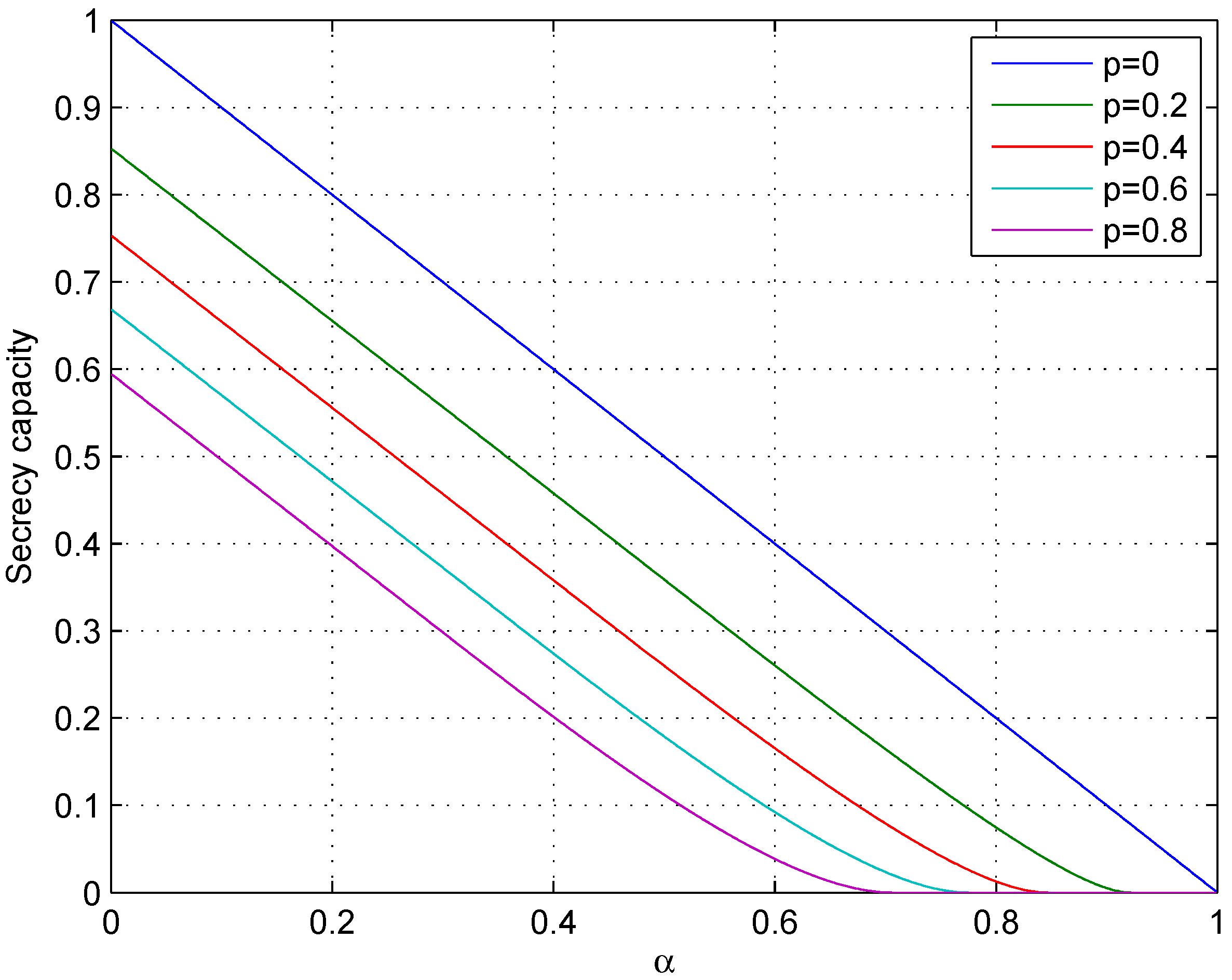
It is clear that when $p=0$, the communication model discussed in this section is specialized as wiretap channel II. In that case, the secrecy capacity is obviously a linear function of α. However, when $p>0$, the linearity does not hold. Instead, the secrecy capacity is a convex function of α. See Figure 6.

6. Conclusions

The paper considers a communication model of extended wiretap channel II. In this new model, the source message is sent to the legitimate receiver through a discrete memoryless channel (DMC), and there exists an eavesdropper who is able to observe the digital sequence from the transmitter through a second DMC. The coding scheme is based on that developed by Ozarow and Wyner for the classic wiretap channel II. This communication model includes the general discrete memoryless wiretap channels, the wiretap channel II and the communication models discussed in [21,22,23] as special cases.

References

- Wyner, A.D. The wire-tap channel. Bell Syst. Tech. J. 1975, 54, 1355–1387. [Google Scholar] [CrossRef]
- Csiszár, I.; Körner, K. Broadcast channels with confidential messages. IEEE Trans. Inf. Theory 1978, 24, 339–348. [Google Scholar] [CrossRef]
- Chen, Y.; Vinck Han, A.J. Wiretap channel with side information. IEEE Trans. Inf. Theory 2008, 54, 395–402. [Google Scholar] [CrossRef]
- Dai, B.; Luo, Y. Some new results on the wiretap channel with side information. Entropy 2012, 14, 1671–1702. [Google Scholar] [CrossRef]
- Dai, B.; Vinck Han, A.J.; Luo, Y.; Zhuang, Z. Degraded Broadcast Vhannel with Noncausal Side Information, Confidential Messages and Noiseless Feedback. In Proceedings of the IEEE International Symposium on Information Theory, Cambridge, MA, USA, 1–6 July 2012.
- Khisti, A.; Diggavi, S.N.; Womell, G.W. Secrete-key agreement with channel state information at the transmitter. IEEE Trans. Inf. Forensics Secur. 2011, 6, 672–681. [Google Scholar] [CrossRef]
- Chia, Y.H.; El Gamal, A. Wiretap channel with causal state information. IEEE Trans. Inf. Theory 2012, 58, 2838–2849. [Google Scholar] [CrossRef]
- Dai, B.; Luo, Y.; Vinck Han, A.J. Capacity Region of Broadcast Channels with Private Message and Causual Side Information. In Proceedings of the 3rd International Congress on Image and Signal Processing, Yantai, China, 16–18 October 2010.
- Liang, Y.; Kramer, G.; Poor, H.; Shamai, S. Compound wiretap channel. EURASIP J. Wirel. Commun. Netw. 2008. [Google Scholar] [CrossRef]
- Bjelaković, I.; Boche, H.; Sommerfeld, J. Capacity results for compound wiretap channels. Probl. Inf. Transm. 2011, 49, 73–98. [Google Scholar] [CrossRef]
- Schaefer, R.F.; Boche, H. Robust broadcasting of common and confidential messages over compound channels: Strong secrecy and decoding performance. IEEE Trans. Inf. Forensics Secur. 2014, 9, 1720–1732. [Google Scholar] [CrossRef]
- Schaefer, R.F.; Loyka, S. The secrecy capacity of compound gaussian MIMO wiretap channels. IEEE Trans. Inf. Theory 2015, 61, 5535–5552. [Google Scholar] [CrossRef]
- Bjelaković, I.; Boche, H.; Sommerfeld, J. Capacity results for arbitrarily varying wiretap channel. Inf. Theory Comb. Search Theory Lect. Notes Comput. Sci. 2013, 7777, 123–144. [Google Scholar]
- Ozarow, L.H.; Wyner, A.D. Wire-tap channel II. AT&T Bell Labs Tech. J. 1984, 63, 2135–2157. [Google Scholar]
- Cai, N.; Yeung, R.W. Secure Network Coding. In Proceedings of the IEEE International Symposium on Information Theory (ISIT), Lausanne, Switzerland, 30 June–5 July 2002.
- Cai, N.; Yeung, R.W. Secure network coding on a wiretap network. IEEE Trans. Inf. Theory 2011, 57, 424–435. [Google Scholar] [CrossRef]
- Feldman, J.; Malkin, T.; Stein, C. On the Capacity of Secure Network Coding. In Proceedings of the 42nd Annual Allerton Conference on Communication, Control, and Computing, Monticello, IL, USA, 29 September–1 October 2004.
- Bhattad, K.; Narayanan, K.R. Weakly secure network coding. Proc. NetCod 2005, 4, 1–5. [Google Scholar]
- Cheng, F.; Yeung, R.W. Performance bounds on a wiretap network with arbitrary wiretap sets. IEEE Trans. Inf. Theory 2012, 60, 3345–3358. [Google Scholar] [CrossRef]
- He, D.; Guo, W. Strong secrecy capacity of a class of wiretap networks. Entropy 2016, 18, 238. [Google Scholar] [CrossRef]
- Nafea, M.; Yener, A. Wiretap Channel II with a Noisy Main Channel. In Proceedings of the IEEE International Symposium on Information Theory (ISIT), Hong Kong, China, 14–19 June 2015.
- Goldfeld, Z.; Cuff, P.; Permuter, H.H. Semantic-security capacity for wiretap channels of type II. IEEE Trans. Inf. Theory 2016, 62, 3863–3879. [Google Scholar] [CrossRef]
- He, D.; Luo, Y.; Cai, N. Strong Secrecy Capacity of the Wiretap Channel II with DMC Main Channel. In Proceedings of the IEEE International Symposium on Information Theory (ISIT), Barcelona, Spain, 10–15 July 2016.
- Luo, Y.; Mitrpant, C.; Vinck Han, A.J. Some new characters on the wiretap channel of type II. IEEE Trans. Inf. Theory 2005, 51, 1222–1229. [Google Scholar] [CrossRef]
- Yang, Y.; Dai, B. A combination of the wiretap channel and the wiretap channel of type II. J. Comput. Inf. Syst. 2014, 10, 4489–4502. [Google Scholar]
- He, D.; Luo, Y. A Kind of Non-DMC Erasure Wiretap Channel. In Proceedings of the IEEE International Conference on Communication Technology (ICCT), Chengdu, China, 9–11 November 2012.
- Kramer, G. Topics in multi-user information theory. Foundations Trends®. Commun. Inf. Theory 2007, 4, 265–444. [Google Scholar]
- Yeung, R.W. Information Theory and Network Coding; Springer: New York, NY, USA, 2008. [Google Scholar]
Figure 1.
Comparison of different secrecy criteria.
Figure 2.
Communication model of wiretap channel II with noise.
Figure 3.
Adding a virtual channel to the communication system.
Figure 4.
Relationship between the function g and β with . (a) ; (b) .
Figure 5.
Parameters achieving the secrecy capacity ().
Figure 6.
Relationship between the secrecy capacity and α.
© 2016 by the authors; licensee MDPI, Basel, Switzerland. This article is an open access article distributed under the terms and conditions of the Creative Commons Attribution (CC-BY) license (http://creativecommons.org/licenses/by/4.0/).
Share and Cite
MDPI and ACS Style
He, D.; Guo, W.; Luo, Y. Secrecy Capacity of the Extended Wiretap Channel II with Noise. Entropy 2016, 18, 377. https://doi.org/10.3390/e18110377
AMA Style
He D, Guo W, Luo Y. Secrecy Capacity of the Extended Wiretap Channel II with Noise. Entropy. 2016; 18(11):377. https://doi.org/10.3390/e18110377
Chicago/Turabian StyleHe, Dan, Wangmei Guo, and Yuan Luo. 2016. "Secrecy Capacity of the Extended Wiretap Channel II with Noise" Entropy 18, no. 11: 377. https://doi.org/10.3390/e18110377
Note that from the first issue of 2016, this journal uses article numbers instead of page numbers. See further details here.