Abstract
We introduce the symplectic structure of information geometry based on Souriau’s Lie group thermodynamics model, with a covariant definition of Gibbs equilibrium via invariances through co-adjoint action of a group on its moment space, defining physical observables like energy, heat, and moment as pure geometrical objects. Using geometric Planck temperature of Souriau model and symplectic cocycle notion, the Fisher metric is identified as a Souriau geometric heat capacity. The Souriau model is based on affine representation of Lie group and Lie algebra that we compare with Koszul works on G/K homogeneous space and bijective correspondence between the set of G-invariant flat connections on G/K and the set of affine representations of the Lie algebra of G. In the framework of Lie group thermodynamics, an Euler-Poincaré equation is elaborated with respect to thermodynamic variables, and a new variational principal for thermodynamics is built through an invariant Poincaré-Cartan-Souriau integral. The Souriau-Fisher metric is linked to KKS (Kostant–Kirillov–Souriau) 2-form that associates a canonical homogeneous symplectic manifold to the co-adjoint orbits. We apply this model in the framework of information geometry for the action of an affine group for exponential families, and provide some illustrations of use cases for multivariate gaussian densities. Information geometry is presented in the context of the seminal work of Fréchet and his Clairaut-Legendre equation. The Souriau model of statistical physics is validated as compatible with the Balian gauge model of thermodynamics. We recall the precursor work of Casalis on affine group invariance for natural exponential families.
Lorsque le fait qu’on rencontre est en opposition avec une théorie régnante, il faut accepter le fait et abandonner la théorie, alors même que celle-ci, soutenue par de grands noms, est généralement adoptée—Claude Bernard in “Introduction à l’Étude de la Médecine Expérimentale” [1]
Au départ, la théorie de la stabilité structurelle m’avait paru d’une telle ampleur et d’une telle généralité, qu’avec elle je pouvais espérer en quelque sorte remplacer la thermodynamique par la géométrie, géométriser en un certain sens la thermodynamique, éliminer des considérations thermodynamiques tous les aspects à caractère mesurable et stochastiques pour ne conserver que la caractérisation géométrique correspondante des attracteurs.—René Thom in “Logos et théorie des Catastrophes” [2]
1. Introduction
This MDPI Entropy Special Issue on “Differential Geometrical Theory of Statistics” collects a limited number of selected invited and contributed talks presented during the GSI’15 conference on “Geometric Science of Information” in October 2015. This paper is an extended version of the paper [3] “Symplectic Structure of Information Geometry: Fisher Metric and Euler-Poincaré Equation of Souriau Lie Group Thermodynamics” published in GSI’15 Proceedings. At GSI’15 conference, a special session was organized on “lie groups and geometric mechanics/thermodynamics”, dedicated to Jean-Marie Souriau’s works in statistical physics, organized by Gery de Saxcé and Frédéric Barbaresco, and an invited talk on “Actions of Lie groups and Lie algebras on symplectic and Poisson manifolds. Application to Lagrangian and Hamiltonian systems” by Charles-Michel Marle, addressing “Souriau’s thermodynamics of Lie groups”. In honor of Jean-Marie Souriau, who died in 2012 and Claude Vallée [4,5,6], who passed away in 2015, this Special Issue will publish three papers on Souriau’s thermodynamics: Marle’s paper on “From Tools in Symplectic and Poisson Geometry to Souriau’s Theories of Statistical Mechanics and Thermodynamics” [7], de Saxcé’s paper on “Link between Lie Group Statistical Mechanics and Thermodynamics of Continua” [8] and this publication by Barbaresco. This paper also proposes new developments, compared to paper [9] where relations between Souriau and Koszul models have been initiated.
This paper, similar to the goal of the papers of Marle and de Saxcé in this Special Issue, is intended to honor the memory of the French Physicist Jean-Marie Souriau and to popularize his works, currently little known, on statistical physics and thermodynamics. Souriau is well known for his seminal and major contributions in geometric mechanics, the discipline he created in the 1960s, from previous Lagrange’s works that he conceptualized in the framework of symplectic geometry, but very few people know or have exploited Souriau’s works contained in Chapter IV of his book “Structure des systèmes dynamiques” published in 1970 [10] and only translated into English in 1995 in the book “Structure of Dynamical Systems: A Symplectic View of Physics” [11], in which he applied the formalism of geometric mechanics to statistical physics. The personal author’s contribution is to place the work of Souriau in the broader context of the emerging “Geometric Science of Information” [12] (addressed in GSI’15 conference), for which the author will show that the Souriau model of statistical physics is particularly well adapted to generalize “information geometry”, that the author illustrates for exponential densities family and multivariate gaussian densities. The author will observe that the Riemannian metric introduced by Souriau is a generalization of Fisher metric, used in “information geometry”, as being identified to the hessian of the logarithm of the generalized partition function (Massieu characteristic function), for the case of densities on homogeneous manifolds where a non-abelian group acts transively. For a group of time translation, we recover the classical thermodynamics and for the Euclidean space, we recover the classical Fisher metric used in Statistics. The author elaborates a new Euler-Poincaré equation for Souriau’s thermodynamics, action on “geometric heat” variable Q (element of dual Lie algebra), and parameterized by “geometric temperature” (element of Lie algebra). The author will integrate Souriau thermodynamics in a variational model by defining an extended Cartan-Poincaré integral invariant defined by Souriau “geometric characteristic function” (the logarithm of the generalized Souriau partition function parameterized by geometric temperature). These results are illustrated for multivariate Gaussian densities, where the associated group is identified to compute a Souriau moment map and reduce the Euler-Poincaré equation of geodesics. In addition, the symplectic cocycle and Souriau-Fisher metric are deduced from a Lie group thermodynamics model.
The main contributions of the author in this paper are the following:
- The Souriau model of Lie group thermodynamics is presented with standard notations of Lie group theory, in place of Souriau equations using less classical conventions (that have limited understanding of his work by his contemporaries).
- We prove that Souriau Riemannian metric introduced with symplectic cocycle is a generalization of Fisher metric (called Souriau-Fisher metric in the following) that preserves the property to be defined as a hessian of partition function logarithm as in classical information geometry. We then establish the equality of two terms, the first one given by Souriau’s definition from Lie group cocycle and parameterized by “geometric heat” Q (element of dual Lie algebra) and “geometric temperature” β (element of Lie algebra) and the second one, the hessian of the characteristic function with respect to the variable β:A dual Souriau-Fisher metric, the inverse of this last one, could be also elaborated with the hessian of “geometric entropy” with respect to the variable Q:For the maximum entropy density (Gibbs density), the following three terms coincide: that describes the convexity of the log-likelihood function, the Fisher metric that describes the covariance of the log-likelihood gradient, whereas that describes the covariance of the observables.
- This Souriau-Fisher metric is also identified to be proportional to the first derivative of the heat , and then comparable by analogy to geometric “specific heat” or “calorific capacity”.
- We observe that the Souriau metric is invariant with respect to the action of the group , due to the fact that the characteristic function after the action of the group is linearly dependent to . As the Fisher metric is proportional to the hessian of the characteristic function, we have the following invariance:
- We have proposed, based on Souriau’s Lie group model and on analogy with mechanical variables, a variational principle of thermodynamics deduced from Poincaré-Cartan integral invariant. The variational principle holds on the Lie algebra, for variations , where is an arbitrary path that vanishes at the endpoints, :where the Poincaré-Cartan integral invariant is defined with , the Massieu characteristic function, with the 1-form
- We have deduced Euler-Poincaré equations for the Souriau model:where is the Souriau geometric heat (element of dual Lie algebra) and is the Souriau geometric temperature (element of the Lie algebra). The second equation is linked to the result of Souriau based on the moment map that a symplectic manifold is always a coadjoint orbit, affine of its group of Hamiltonian transformations (a symplectic manifold homogeneous under the action of a Lie group, is isomorphic, up to a covering, to a coadjoint orbit; symplectic leaves are the orbits of the affine action that makes the moment map equivariant).
- We have established that the affine representation of Lie group and Lie algebra by Jean-Marie Souriau is equivalent to Jean-Louis Koszul’s affine representation developed in the framework of hessian geometry of convex sharp cones. Both Souriau and Koszul have elaborated equations requested for Lie group and Lie algebra to ensure the existence of an affine representation. We have compared both approaches of Souriau and Koszul in a table.
- We have applied the Souriau model for exponential families and especially for multivariate Gaussian densities.
- We have applied the Souriau-Koszul model Gibbs density to compute the maximum entropy density for symmetric positive definite matrices, using the inner product , given by Cartan-Killing form. The Gibbs density (generalization of Gaussian law for theses matrices and defined as maximum entropy density):
- For the case of multivariate Gaussian densities, we have considered a sub-group of affine group, that we defined by a (n + 1) × (n + 1) embedding in matrix Lie group , and that acts for multivariate Gaussian laws by:
- For multivariate Gaussian densities, as we have identified the acting sub-group of affine group , we have also developed the computation of the associated Lie algebras and , adjoint and coadjoint operators, and especially the Souriau “moment map” :Using Souriau Theorem (geometrization of Noether theorem), we use the property that this moment map is constant (its components are equal to Noether invariants):to reduce the Euler-Lagrange equation of geodesics between two multivariate Gaussian densities:to this reduced equation of geodesics:that we solve by “geodesic shooting” technic based on Eriksen equation of exponential map.
- For the families of multivariate Gaussian densities, that we have identified as homogeneous manifold with the associated sub-group of the affine group , we have considered the elements of exponential families, that play the role of geometric heat in Souriau Lie group thermodynamics, and the geometric (Planck) temperature:We have considered that these elements are homeomorph to the (n + 1) × (n + 1) matrix elements:to compute the Souriau symplectic cocycle of the Lie group:where the adjoint operator is equal to:withand the co-adjoint operator:
- Finally, we have computed the Souriau-Fisher metric for multivariate Gaussian densities, given by:with element of Lie algebra given by .
The plan of the paper is as follows. After this introduction in Section 1, we develop in Section 2 the position of Souriau symplectic model of statistical physics in the historical developments of thermodynamic concepts. In Section 3, we develop and revisit the Lie group thermodynamics model of Jean-Marie Souriau in modern notations. In Section 4, we make the link between Souriau Riemannian metric and Fisher metric defined as a geometric heat capacity of Lie group thermodynamics. In Section 5, we elaborate Euler-Lagrange equations of Lie group thermodynamics and a variational model based on Poincaré-Cartan integral invariant. In Section 6, we explore Souriau affine representation of Lie group and Lie algebra (including the notions of: affine representations and cocycles, Souriau moment map and cocycles, equivariance of Souriau moment map, action of Lie group on a symplectic manifold and dual spaces of finite-dimensional Lie algebras) and we analyze the link and parallelisms with Koszul affine representation, developed in another context (comparison is synthetized in a table). In Section 7, we illustrate Koszul and Souriau Lie group models of information geometry for multivariate Gaussian densities. In Section 8, after identifying the affine group acting for these densities, we compute the Souriau moment map to obtain the Euler-Poincaré equation, solved by geodesic shooting method. In Section 9, Souriau Riemannian metric defined by cocycle for multivariate Gaussian densities is computed. We give a conclusion in Section 10 with research prospects in the framework of affine Poisson geometry [13], Bismut stochastic mechanics [14] and second order extension of the Gibbs state [15,16]. We have three appendices: Appendix A develops the Clairaut(-Legendre) equation of Maurice Fréchet associated to “distinguished functions” as a seminal equation of information geometry; Appendix B is about a Balian Gauge model of thermodynamics and its compliance with the Souriau model; Appendix C is devoted to the link of Casalis-Letac’s works on affine group invariance for natural exponential families with Souriau’s works.
2. Position of Souriau Symplectic Model of Statistical Physics in Historical Developments of Thermodynamic Concepts
In this Section, we will explain the emergence of thermodynamic concepts that give rise to the generalization of the Souriau model of statistical physics. To understand Souriau’s theoretical model of heat, we have to consider first his work in geometric mechanics where he introduced the concept of “moment map” and “symplectic cohomology”. We will then introduce the concept of “characteristic function” developed by François Massieu, and generalized by Souriau on homogeneous symplectic manifolds. In his statistical physics model, Souriau has also generalized the notion of “heat capacity” that was initially extended by Pierre Duhem as a key structure to jointly consider mechanics and thermodynamics under the umbrella of the same theory. Pierre Duhem has also integrated, in the corpus, the Massieu’s characteristic function as a thermodynamic potential. Souriau’s idea to develop a covariant model of Gibbs density on homogeneous manifold was also influenced by the seminal work of Constantin Carathéodory that axiomatized thermodynamics in 1909 based on Carnot’s works. Souriau has adapted his geometric mechanical model for the theory of heat, where Henri Poincaré did not succeed in his paper on attempts of mechanical explanation for the principles of thermodynamics.
Lagrange’s works on “mécanique analytique (analytic mechanics)” has been interpreted by Jean-Marie Souriau in the framework of differential geometry and has initiated a new discipline called after Souriau, “mécanique géométrique (geometric mechanics)” [17,18,19]. Souriau has observed that the collection of motions of a dynamical system is a manifold with an antisymmetric flat tensor that is a symplectic form where the structure contains all the pertinent information of the state of the system (positions, velocities, forces, etc.). Souriau said: “Ce que Lagrange a vu, que n’a pas vu Laplace, c’était la structure symplectique (What Lagrange saw, that Laplace didn’t see, was the symplectic structure” [20]. Using the symmetries of a symplectic manifold, Souriau introduced a mapping which he called the “moment map” [21,22,23], which takes its values in a space attached to the group of symmetries (in the dual space of its Lie algebra). He [10] called dynamical groups every dimensional group of symplectomorphisms (an isomorphism between symplectic manifolds, a transformation of phase space that is volume-preserving), and introduced Galileo group for classical mechanics and Poincaré group for relativistic mechanics (both are sub-groups of affine group [24,25]). For instance, a Galileo group could be represented in a matrix form by (with A rotation, b the boost, c space translation and e time translation):
Souriau associated to this moment map, the notion of symplectic cohomology, linked to the fact that such a moment is defined up to an additive constant that brings into play an algebraic mechanism (called cohomology). Souriau proved that the moment map is a constant of the motion, and provided geometric generalization of Emmy Noether invariant theorem (invariants of E. Noether theorem are the components of the moment map). For instance, Souriau gave an ontological definition of mass in classical mechanics as the measure of the symplectic cohomology of the action of the Galileo group (the mass is no longer an arbitrary variable but a characteristic of the space). This is no longer true for Poincaré group in relativistic mechanics, where the symplectic cohomology is null, explaining the lack of conservation of mass in relativity. All the details of classical mechanics thus appear as geometric necessities, as ontological elements. Souriau has also observed that the symplectic structure has the property to be able to be reconstructed from its symmetries alone, through a 2-form (called Kirillov–Kostant–Souriau form) defined on coadjoint orbits. Souriau said that the different versions of mechanical science can be classified by the geometry that each implies for space and time; geometry is determined by the covariance of group theory. Thus, Newtonian mechanics is covariant by the group of Galileo, the relativity by the group of Poincaré; General relativity by the “smooth” group (the group of diffeomorphisms of space-time). However, Souriau added “However, there are some statements of mechanics whose covariance belongs to a fourth group rarely considered: the affine group, a group shown in the following diagram for inclusion. How is it possible that a unitary point of view (which would be necessarily a true thermodynamics), has not yet come to crown the picture? Mystery...” [26]. See Figure 1.
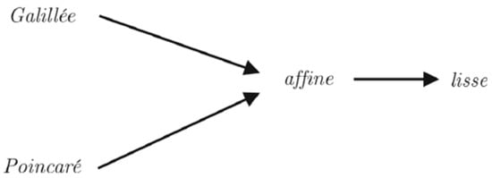
Figure 1.
Souriau Scheme about mysterious “affine group” of a true thermodynamics between Galileo group of classical mechanics, Poincaré group of relativistic mechanics and Smooth group of general relativity.
As early as 1966, Souriau applied his theory to statistical mechanics, developed it in the Chapter IV of his book “Structure of Dynamical Systems” [11], and elaborated what he called a “Lie group thermodynamics” [10,11,27,28,29,30,31,32,33,34,35,36,37]. Using Lagrange’s viewpoint, in Souriau statistical mechanics, a statistical state is a probability measure on the manifold of motions (and no longer in phase space [38]). Souriau observed that Gibbs equilibrium [39] is not covariant with respect to dynamic groups of Physics. To solve this braking of symmetry, Souriau introduced a new “geometric theory of heat” where the equilibrium states are indexed by a parameter with values in the Lie algebra of the group, generalizing the Gibbs equilibrium states, where plays the role of a geometric (Planck) temperature. The invariance with respect to the group, and the fact that the entropy is a convex function of this geometric temperature , imposes very strict, universal conditions (e.g., there exists necessarily a critical temperature beyond which no equilibrium can exist). Souriau observed that the group of time translations of the classical thermodynamics [40,41] is not a normal subgroup of the Galilei group, proving that if a dynamical system is conservative in an inertial reference frame, it need not be conservative in another. Based on this fact, Souriau generalized the formulation of the Gibbs principle to become compatible with Galileo relativity in classical mechanics and with Poincaré relativity in relativistic mechanics. The maximum entropy principle [42,43,44,45,46,47,48,49,50,51] is preserved, and the Gibbs density is given by the density of maximum entropy (among the equilibrium states for which the average value of the energy takes a prescribed value, the Gibbs measures are those which have the largest entropy), but with a new principle “If a dynamical system is invariant under a Lie subgroup G’ of the Galileo group, then the natural equilibria of the system forms the Gibbs ensemble of the dynamical group G’” [10]. The classical notion of Gibbs canonical ensemble is extended for a homogneous symplectic manifold on which a Lie group (dynamic group) has a symplectic action. When the group is not abelian (non-commutative group), the symmetry is broken, and new “cohomological” relations should be verified in Lie algebra of the group [52,53,54,55]. A natural equilibrium state will thus be characterized by an element of the Lie algebra of the Lie group, determining the equilibrium temperature . The entropy , parametrized by the geometric heat (mean of energy , element of the dual Lie algebra) is defined by the Legendre transform [56,57,58,59] of the Massieu potential parametrized by ( is the minus logarithm of the partition function ):
Souriau completed his “geometric heat theory” by introducing a 2-form in the Lie algebra, that is a Riemannian metric tensor in the values of adjoint orbit of , with an element of the Lie algebra. This metric is given for :
where is a cocycle of the Lie algebra, defined by with a cocycle of the Lie group defined by . We have observed that this metric is also given by the hessian of the Massieu potential as Fisher metric in classical information geometry theory [60], and so this is a generalization of the Fisher metric for homogeneous manifold. We call this new metric the Souriau-Fisher metric. As , Souriau compared it by analogy with classical thermodynamics to a “geometric specific heat” (geometric calorific capacity).
The potential theory of thermodynamics and the introduction of “characteristic function” (previous function in Souriau theory) was initiated by François Jacques Dominique Massieu [61,62,63,64]. Massieu was the son of Pierre François Marie Massieu and Thérèse Claire Castel. He married in 1862 with Mlle Morand and had 2 children. He graduated from Ecole Polytechnique in 1851 and Ecole des Mines de Paris in 1956, he has integrated “Corps des Mines”. He defended his Ph.D. in 1861 on “Sur les intégrales algébriques des problèmes de mécanique” and on “Sur le mode de propagation des ondes planes et la surface de l’onde élémentaire dans les cristaux biréfringents à deux axes” [65] with the jury composed of Lamé, Delaunay et Puiseux. In 1870, François Massieu presented his paper to the French Academy of Sciences on “characteristic functions of the various fluids and the theory of vapors” [61]. The design of the characteristic function is the finest scientific title of Mr. Massieu. A prominent judge, Joseph Bertrand, do not hesitate to declare, in a statement read to the French Academy of Sciences 25 July 1870, that “the introduction of this function in formulas that summarize all the possible consequences of the two fundamental theorems seems, for the theory, a similar service almost equivalent to that Clausius has made by linking the Carnot’s theorem to entropy” [66]. The final manuscript was published by Massieu in 1873, “Exposé des principes fondamentaux de la théorie mécanique de la chaleur (Note destinée à servir d’introduction au Mémoire de l’auteur sur les fonctions caractéristiques des divers fluides et la théorie des vapeurs)” [63].
Massieu introduced the following potential , called “characteristic function”, as illustrated in Figure 2, that is the potential used by Souriau to generalize the theory: . However, in his third paper, Massieu was influenced by M. Bertrand, as illustrated in Figure 3, to replace the variable (that he used in his two first papers) by . We have then to wait 50 years more for the paper of Planck, who introduced again the good variable , and then generalized by Souriau, giving to Planck temperature an ontological and geometric status as element of the Lie algebra of the dynamic group.
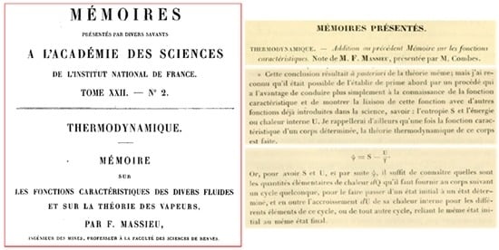
Figure 2.
Extract from the second paper of François Massieu to the French Academy of Sciences [61,62].
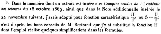
Figure 3.
Remark of Massieu in 1876 paper [64], where he explained why he took into account the “good advice” of Bertrand to replace variable 1/T, used in his initial paper of 1869, by the variable T.
This Lie group thermodynamics of Souriau is able to explain astronomical phenomenon (rotation of celestial bodies: the Earth and the stars rotating about themselves). The geometric temperature can be also interpreted as a space-time vector (generalization of the temperature vector of Planck), where the temperature vector and entropy flux are in duality unifying heat conduction and viscosity (equations of Fourier and Navier). In case of centrifuge system (e.g., used for enrichment of uranium), the Gibbs Equilibrium state [60,67] are given by Souriau equations as the variation in concentration of the components of an inhomogeneous gas. Classical statistical mechanics corresponds to the dynamical group of time translations, for which we recover from Souriau equations the concepts and principles of classical thermodynamics (temperature, energy, heat, work, entropy, thermodynamic potentials) and of the kinetic theory of gases (pressure, specific heats, Maxwell’s velocity distribution, etc.).
Souriau also studied continuous medium thermodynamics, where the “temperature vector” is no longer constrained to be in Lie algebra, but only contrained by phenomenologic equations (e.g., Navier equations, etc.). For thermodynamic equilibrium, the “temperature vector” is then a Killing vector of Space-Time. For each point X, there is a “temperature vector” , such it is an infinitesimal conformal transform of the metric of the universe . Conservation equations can then be deduced for components of impulsion-energy tensor and entropy flux with . Temperature and metric are related by the following equations:
Leon Brillouin made the link between Boltzmann entropy and Negentropie of information theory [68,69,70,71], but before Jean-Marie Souriau, only Constantin Carathéodory and Pierre Duhem [72,73,74,75] initiated first theoretical works to generalize thermodynamics.
After three years as lecturer at Lille university, Duhem published a paper in the official revue of the Ecole Normale Supérieure, in 1891, “On general equations of thermodynamics” [72] (Sur les équations générales de la Thermodynamique) in Annales Scientifiques de l’Ecole Normale Supérieure. Duhem generalized the concept of “virtual work” under the action of “external actions” by taking into account both mechanical and thermal actions. In 1894, the design of a generalized mechanics based on thermodynamics was further developed: ordinary mechanics had already become “a particular case of a more general science”. Duhem writes “We made dynamics a special case of thermodynamics, a science that embraces common principles in all changes of state bodies, changes of places as well as changes in physical qualities” (Nous avons fait de la dynamique un cas particulier de la thermodynamique, une Science qui embrasse dans des principes communs tous les changements d’état des corps, aussi bien les changements de lieu que les changements de qualités physiques). In the equations of his generalized mechanics-thermodynamics, some new terms had to be introduced, in order to account for the intrinsic viscosity and friction of the system. As observed by Stefano Bordoni, Duhem aimed at widening the scope of physics: the new physics could not confine itself to “local motion” but had to describe what Duhem qualified “motions of modification”. If Boltzmann had tried to proceed from “local motion” to attain the explanation of more complex transformations, Duhem was trying to proceed from general laws concerning general transformation in order to reach “local motion” as a simplified specific case. Four scientists were credited by Duhem with having carried out “the most important researches on that subject”: Massieu had managed to derive thermodynamics from a “characteristic function and its partial derivatives”; Gibbs had shown that Massieu’s functions “could play the role of potentials in the determination of the states of equilibrium” in a given system; von Helmholtz had put forward “similar ideas”; von Oettingen had given “an exposition of thermodynamics of remarkable generality” based on general duality concept in “Die thermodynamischen Beziehungen antithetisch entwickelt” published at St. Petersburg in 1885. Duhem took into account a system whose elements had the same temperature and where the state of the system could be completely specified by giving its temperature and n other independent quantities. He then introduced some “external forces”, and held the system in equilibrium. A virtual work corresponded to such forces, and a set of n + 1 equations corresponded to the condition of equilibrium of the physical system. From the thermodynamic point of view, every infinitesimal transformation involving the generalized displacements had to obey to the first law, which could be expressed in terms of the (n + 1) generalized Lagrangian parameters. The amount of heat could be written as a sum of (n + 1) terms. The new alliance between mechanics and thermodynamics led to a sort of symmetry between thermal and mechanical quantities. The n + 1 functions played the role of generalized thermal capacities, and the last term was nothing other than the ordinary thermal capacity. The knowledge of the “equilibrium equations of a system” allowed Duhem to compute the partial derivatives of the thermal capacity with regard to all the parameters which described the state of the system, apart from its derivative with regard to temperature. The thermal capacities were therefore known “except for an unspecified function of temperature”.
The axiomatic approach of thermodynamics was published in 1909 in Mathematische Annalen [76] under the title “Examination of the Foundations of Thermodynamics” (Untersuchungen überdie Grundlagen der Thermodynamik) by Constantin Carathéodory based on Carnot’s works [77]. Carathéodory introduced entropy through a mathematical approach based on the geometric behavior of a certain class of partial differential equations called Pfaffians. Carathéodory’s investigations start by revisiting the first law and reformulating the second law of thermodynamics in the form of two axioms. The first axiom applies to a multiphase system change under adiabatic conditions (axiom of classical thermodynamics due to Clausius [78,79]). The second axiom assumes that in the neighborhood of any equilibrium state of a system (of any number of thermodynamic coordinates), there exist states that are inaccessible by reversible adiabatic processes. In the book of Misha Gromov “Metric Structures for Riemannian and Non-Riemannian Spaces”, written and edited by Pierre Pansu and Jacques Lafontaine, a new metric is introduced called “Carnot-Carathéodory metric”. In one of his papers, Misha Gromov [80,81] gives historical remarks “This result (which seems obvious by the modern standards) appears (in a more general form) in the 1909-paper by Carathéorody on formalization of the classical thermodynamics where horizontal curves roughly correspond to adiabatic processes. In fact, the above proof may be performed in the language of Carnot (cycles) and for this reason the metris distH were christened ‘Carnot-Carathéodory’ in Gromov-Lafontaine-Pansu book” [82]. When I ask this question to Pierre Pansu, he gave me the answer that “The section 4 of [76], entitled Hilfsatz aus der Theorie des Pfaffschen Gleichungen (Lemma from the theory of Pfaffian equations) opens with a statement relating to the differential 1-forms. Carathéodory says, If a Pfaffian equation dx0 + X1 dx1 + X2 dx2 + … + Xn dxn = 0 is given, in which the Xi are finite, continuous, differentiable functions of the xi, and one knows that in any neighborhood of an arbitrary point P of the space of xi there is a point that one cannot reach along a curve that satisfies this equation then the expression must necessarily possess a multiplier that makes it into a complete differential”. This is confirmed in the introduction of his paper [76], where Carathéodory said “Finally, in order to be able to treat systems with arbitrarily many degrees of freedom from the outset, instead of the Carnot cycle that is almost always used, but is intuitive and easy to control only for systems with two degrees of freedom, one must employ a theorem from the theory of Pfaffian differential equations, for which a simple proof is given in the fourth section”.
We have also to make reference to Henri Poincaré [83] that published the paper “On attempts of mechanical explanation for the principles of thermodynamics (Sur les tentatives d’explication mécanique des principes de la thermodynamique)” at the Comptes rendus de l’Académie des sciences in 1889 [84], in which he tried to consolidate links between mechanics and thermomechanics principles. These elements were also developed in Poincaré’s lecture of 1892 [85] on “thermodynamique” in Chapter XVII “Reduction of thermodynamics principles to the general principles of mechanics (Réduction des principes de la Thermodynamique aux principes généraux de la mécanique)”. Poincaré writes in his book [85] “It is otherwise with the second law of thermodynamics. Clausius was the first to attempt to bring it to the principles of mechanics, but not succeed satisfactorily. Helmholtz in his memoir on the principle of least actions developed a theory much more perfect than that of Clausius. However, it cannot account for irreversible phenomena. (Il en est autrement du second principe de la thermodynamique. Clausius, a le premier, tenté de le ramener aux principes de la Mécanique, mais sans y réussir d’une manière satisfaisante. Helmoltz dans son mémoire sur le principe de la moindre action, a développé une théorie beaucoup plus parfaite que celle de Clausius; cependant elle ne peut rendre compte des phénomènes irréversibles.)”. About Helmoltz work, Poincaré observes [85] “It follows from these examples that the Helmholtz hypothesis is true in the case of body turning around an axis; So it seems applicable to vortex motions of molecules (Il résulte de ces exemples que l’hypothèse d’Helmoltz est exacte dans le cas de corps tournant autour d’un axe; elle parait donc applicable aux mouvements tourbillonnaires des molecules.)”, but he adds in the following that the Helmoltz model is also true in the case of vibrating motions as molecular motions. However, he finally observes that the Helmoltz model cannot explain the increasing of entropy and concludes [85] “All attempts of this nature must be abandoned; the only ones that have any chance of success are those based on the intervention of statistical laws, for example, the kinetic theory of gases. This view, which I cannot develop here, can be summed up in a somewhat vulgar way as follows: Suppose we want to place a grain of oats in the middle of a heap of wheat; it will be easy; then suppose we wanted to find it and remove it; we cannot achieve it. All irreversible phenomena, according to some physicists, would be built on this model (Toutes les tentatives de cette nature doivent donc être abandonnées; les seules qui aient quelque chance de succès sont celles qui sont fondées sur l’intervention des lois statistiques comme, par exemple, la théorie cinétique des gaz. Ce point de vue, que je ne puis développer ici, peut se résumer d’une façon un peu vulgaire comme il suit: Supposons que nous voulions placer un grain d’avoine au milieu d’un tas de blé; cela sera facile; supposons que nous voulions ensuite l’y retrouver et l’en retirer; nous ne pourrons y parvenir. Tous les phénomènes irréversibles, d’après certains physiciens, seraient construits sur ce modèle)”. In Poincaré’s lecture, Massieu has greatly influenced Poincaré to introduce Massieu characteristic function in probability [86]. As we have observed, Poincaré has introduced characteristic function in probability lecture after his lecture on thermodynamics where he discovered in its second edition [85], the Massieu’s characteristic function. We can read that “Since from the functions of Mr. Massieu one can deduce other functions of variables, all equations of thermodynamics can be written so as to only contain these functions and their derivatives; it will thus result in some cases, a great simplification (Puisque des fonctions de M. Massieu on peut déduire les autres fonctions des variables, toutes les équations de la Thermodynamique pourront s’écrire de manière à ne plus renfermer que ces fonctions et leurs dérivées; il en résultera donc, dans certains cas, une grande simplification).” [85]. He [85] added “MM. Gibbs von Helmholtz, Duhem have used this function H = U − TS assuming that T and V are constant. Mr. von Helmotz has called it ‘free energy’ and also proposes to give him the name of “kinetic potential”; Duhem called it ‘the thermodynamic potential at constant volume’; this is the most justified naming (MM. Gibbs, von Helmoltz, Duhem ont fait usage de cette function H = TS − U en y supposant T et V constants. M. von Helmotz l’a appellée énergie libre et a propose également de lui donner le nom de potential kinetique; M. Duhem la nomme potentiel thermodynamique à volume constant; c’est la dénomination la plus justifiée)”. In 1906, Henri Poincaré also published a note [87] “Reflection on The kinetic theory of gases” (Réflexions sur la théorie cinétique des gaz), where he said that: “The kinetic theory of gases leaves awkward points for those who are accustomed to mathematical rigor … One of the points which embarrassed me most was the following one: it is a question of demonstrating that the entropy keeps decreasing, but the reasoning of Gibbs seems to suppose that having made vary the outside conditions we wait that the regime is established before making them vary again. Is this supposition essential, or in other words, we could arrive at opposite results to the principle of Carnot by making vary the outside conditions too fast so that the permanent regime has time to become established?”.
Jean-Marie Souriau has elaborated a disruptive and innovative “théorie géométrique de la chaleur (geometric theory of heat)” [88] after the works of his predecessors as illustrated in Figure 4: “théorie analytique de la chaleur (analytic theory of heat)” by Jean Baptiste Joseph Fourier [88], “théorie mécanique de la chaleur (mechanic theory of heat)” by François Clausius [89] and François Massieu and “théorie mathématique de la chaleur (mathematic theory of heat)” by Siméon-Denis Poisson [90,91], as illustrated in this figure:
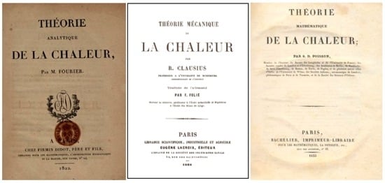
Figure 4.
“Théorie analytique de la chaleur (analytic theory of heat)” by Jean Baptiste Joseph Fourier [88], “théorie mécanique de la chaleur (mechanic theory of heat)” by François Clausius [89] and “théorie mathématique de la chaleur (mathematic theory of heat)” by Siméon-Denis Poisson [90].
3. Revisited Souriau Symplectic Model of Statistical Physics
In this Section, we will revisit the Souriau model of thermodynamics but with modern notations, replacing personal Souriau conventions used in his book of 1970 by more classical ones.
In 1970, Souriau introduced the concept of co-adjoint action of a group on its momentum space (or “moment map”: mapping induced by symplectic manifold symmetries), based on the orbit method works, that allows to define physical observables like energy, heat and momentum or moment as pure geometrical objects (the moment map takes its values in a space determined by the group of symmetries: the dual space of its Lie algebra). The moment(um) map is a constant of the motion and is associated to symplectic cohomology (assignment of algebraic invariants to a topological space that arises from the algebraic dualization of the homology construction). Souriau introduced the moment map in 1965 in a lecture notes at Marseille University and published it in 1966. Souriau gave the formal definition and its name based on its physical interpretation in 1967. Souriau then studied its properties of equivariance, and formulated the coadjoint orbit theorem in his book in 1970. However, in his book, Souriau also observed in Chapter IV that Gibbs equilibrium states are not covariant by dynamical groups (Galileo or Poincaré groups) and then he developed a covariant model that he called “Lie group thermodynamics”, where equilibriums are indexed by a “geometric (Planck) temperature”, given by a vector that lies in the Lie algebra of the dynamical group. For Souriau, all the details of classical mechanics appear as geometric necessities (e.g., mass is the measure of the symplectic cohomology of the action of a Galileo group). Based on this new covariant model of thermodynamic Gibbs equilibrium, Souriau has formulated statistical mechanics and thermodynamics in the framework of symplectic geometry by use of symplectic moments and distribution-tensor concepts, giving a geometric status for temperature, heat and entropy.
There is a controversy about the name “momentum map” or “moment map”. Smale [92] referred to this map as the “angular momentum”, while Souriau used the French word “moment”. Cushman and Duistermaat [93] have suggested that the proper English translation of Souriau’s French word was “momentum” which fit better with standard usage in mechanics. On the other hand, Guillemin and Sternberg [94] have validated the name given by Souriau and have used “moment” in English. In this paper, we will see that name “moment” given by Souriau was the most appropriate word. In his Chapter IV of his book [10], studying statistical mechanics, Souriau [10] has ingeniously observed that moments of inertia in mechanics are equivalent to moments in probability in his new geometric model of statistical physics. We will see that in Souriau Lie group thermodynamic model, these statistical moments will be given by the energy and the heat defined geometrically by Souriau, and will be associated with “moment map” in dual Lie algebra.
This work has been extended by Claude Vallée [5,6] and Gery de Saxcé [4,8,95,96]. More recently, Kapranov has also given a thermodynamical interpretation of the moment map for toric varieties [97] and Pavlov, thermodynamics from the differential geometry standpoint [98].
The conservation of the moment of a Hamiltonian action was called by Souriau the “symplectic or geometric Noether theorem”. Considering phases space as symplectic manifold, cotangent fiber of configuration space with canonical symplectic form, if Hamiltonian has Lie algebra, then the moment map is constant along the system integral curves. Noether theorem is obtained by considering independently each component of the moment map.
In a first step to establish new foundations of thermodynamics, Souriau [10] has defined a Gibbs canonical ensemble on a symplectic manifold M for a Lie group action on M. In classical statistical mechanics, a state is given by the solution of Liouville equation on the phase space, the partition function. As symplectic manifolds have a completely continuous measure, invariant by diffeomorphisms, the Liouville measure λ, all statistical states will be the product of the Liouville measure by the scalar function given by the generalized partition function defined by the energy (defined in the dual of the Lie algebra of this dynamical group) and the geometric temperature , where is a normalizing constant such the mass of probability is equal to 1, [99]. Jean-Marie Souriau then generalizes the Gibbs equilibrium state to all symplectic manifolds that have a dynamical group. To ensure that all integrals that will be defined could converge, the canonical Gibbs ensemble is the largest open proper subset (in Lie algebra) where these integrals are convergent. This canonical Gibbs ensemble is convex. The derivative of , (thermodynamic heat) is equal to the mean value of the energy . The minus derivative of this generalized heat , is symmetric and positive (this is a geometric heat capacity). Entropy is then defined by Legendre transform of , . If this approach is applied for the group of time translation, this is the classical thermodynamics theory. However, Souriau [10] has observed that if we apply this theory for non-commutative group (Galileo or Poincaré groups), the symmetry has been broken. Classical Gibbs equilibrium states are no longer invariant by this group. This symmetry breaking provides new equations, discovered by Souriau [10].
We can read in his paper this prophetical sentence “This Lie group thermodynamics could be also of first interest for mathematics (Peut-être cette Thermodynamique des groups de Lie a-t-elle un intérêt mathématique)” [30]. He explains that for the dynamic Galileo group with only one axe of rotation, this thermodynamic theory is the theory of centrifuge where the temperature vector dimension is equal to 2 (sub-group of invariance of size 2), used to make “uranium 235” and “ribonucleic acid” [30]. The physical meaning of these two dimensions for vector-valued temperature is “thermic conduction” and “viscosity”. Souriau said that the model unifies “heat conduction” and “viscosity” (Fourier and Navier equations) in the same theory of irreversible process. Souriau has applied this theory in detail for relativistic ideal gas with the Poincaré group for the dynamical group.
Before introducing the Souriau Model of Lie group thermodynamics, we will first remind readers of the classical notation of Lie group theory in their application to Lie group thermodynamics:
- The coadjoint representation of is the contragredient of the adjoint representation. It associates to each the linear isomorphism , which satisfies, for each and :
- The adjoint representation of the Lie algebra is the linear representation of into itself which associates, to each , the linear map . Tangent application of at neutral element of :
- The coadjoint representation of the Lie algebra is the contragredient of the adjoint representation. It associates, to each , the linear map which satisfies, for each and :We can illustrate for group of matrices for with .Then, the curve from tangent to is given by and transform by :For each temperature , element of the Lie algebra , Souriau has introduced a tensor , equal to the sum of the cocycle and the heat coboundary (with [.,.] Lie bracket):This tensor has the following properties:
- where the map is the one-cocycle of the Lie algebra with values in , with where the one-cocycle of the Lie group G. is constant on M and the map is a skew-symmetric bilinear form, and is called the symplectic cocycle of Lie algebra associated to the moment map , with the following properties:where linear application from to differential function on : and the associated differentiable application , called moment(um) map:If instead of we take the following moment map:where is constant, the symplectic cocycle is replaced bywhere is one-coboundary of with values in . We also have properties and .
- The geometric temperature, element of the algebra , is in the thekernel of the tensor :
- The following symmetric tensor , defined on all values of is positive definite:where the linear map is the adjoint representation of the Lie algebra defined by , and the co-adjoint representation of the Lie algebra the linear map which satisfies, for each and :These equations are universal, because they are not dependent on the symplectic manifold but only on the dynamical group G, the symplectic cocycle , the temperature and the heat . Souriau called this model “Lie groups thermodynamics”.
We will give the main theorem of Souriau for this “Lie group thermodynamics”:
Theorem 1 (Souriau Theorem of Lie Group Thermodynamics).
Let be the largest open proper subset of , Lie algebra of G, such that and are convergent integrals, this set is convex and is invariant under every transformation , where is the adjoint representation of G, such that with . Let a unique affine action such that linear part is a coadjoint representation of , that is the contragradient of the adjoint representation. It associates to each the linear isomorphism , satisfying, for each:
Then, the fundamental equations of Lie group thermodynamics are given by the action of the group:
- Action of Lie group on Lie algebra:
- Transformation of characteristic function after action of Lie group:
- Invariance of entropy with respect to action of Lie group:
- Action of Lie group on geometric heat, element of dual Lie algebra:
Souriau equations of Lie group thermodynamics are summarized in the following Figure 5 and Figure 6:
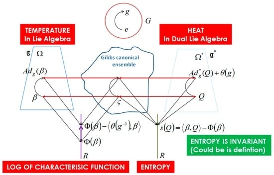
Figure 5.
Global Souriau scheme of Lie group thermodynamics.
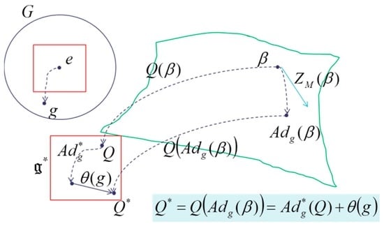
Figure 6.
Broken symmetry on geometric heat Q due to adjoint action of the group on temperature β as an element of the Lie algebra.
For Hamiltonian, actions of a Lie group on a connected symplectic manifold, the equivariance of the moment map with respect to an affine action of the group on the dual of its Lie algebra has been studied by Marle and Libermann [100] and Lichnerowics [101,102]:
Theorem 2 (Marle Theorem on Cocycles).
Let be a connected and simply connected Lie group, be a linear representation of in a finite-dimensional vector space E, and be the associated linear representation of its Lie algebra . For any one-cocycle of the Lie algebra for the linear representation r, there exists a unique one-cocycle of the Lie group for the linear representation R such that , which has as associated Lie algebra one-cocycle. The Lie group one-cocycle is a Lie group one-coboundary if and only if the Lie algebra one-cocycle is a Lie algebra one-coboundary.
Let be a Lie group whose Lie algebra is . The skew-symmetric bilinear form on can be extended into a closed differential two-form on , since the identity on means that its exterior differential vanishes. In other words, is a 2-cocycle for the restriction of the de Rham cohomology of to left invariant differential forms. In the framework of Lie group action on a symplectic manifold, equivariance of moment could be studied to prove that there is a unique action a(.,.) of the Lie group on the dual of its Lie algebra for which the moment map is equivariant, that means for each :
where is an action of Lie group G on differentiable manifold M, the fundamental field associated to an element of Lie algebra of group G is the vectors field on M:
with and . is Hamiltonian on a symplectic manifold , if is symplectic and if for all , the fundamental field is globally Hamiltonian. The cohomology class of the symplectic cocycle only depends on the Hamiltonian action , and not on .
In Appendix B, we observe that Souriau Lie group thermodynamics is compatible with Balian gauge theory of thermodynamics [103], that is obtained by symplectization in dimension 2n + 2 of contact manifold in dimension 2n + 1. All elements of the Souriau geometric temperature vector are multiplied by the same gauge parameter.
We conclude this section by this Bourbakiste citation of Jean-Marie Souriau [34]:
It is obvious that one can only define average values on objects belonging to a vector (or affine) space; Therefore—so this assertion may seem Bourbakist—that we will observe and measure average values only as quantity belonging to a set having physically an affine structure. It is clear that this structure is necessarily unique—if not the average values would not be well defined. (Il est évident que l’on ne peut définir de valeurs moyennes que sur des objets appartenant à un espace vectoriel (ou affine); donc—si bourbakiste que puisse sembler cette affirmation—que l’on n’observera et ne mesurera de valeurs moyennes que sur des grandeurs appartenant à un ensemble possédant physiquement une structure affine. Il est clair que cette structure est nécessairement unique—sinon les valeurs moyennes ne seraient pas bien définies.).
4. The Souriau-Fisher Metric as Geometric Heat Capacity of Lie Group Thermodynamics
We observe that Souriau Riemannian metric, introduced with symplectic cocycle, is a generalization of the Fisher metric, that we call the Souriau-Fisher metric, that preserves the property to be defined as a hessian of the partition function logarithm as in classical information geometry. We will establish the equality of two terms, between Souriau definition based on Lie group cocycle and parameterized by “geometric heat” Q (element of dual Lie algebra) and “geometric temperature” β (element of Lie algebra) and hessian of characteristic function with respect to the variable β:
If we differentiate this relation of Souriau theorem , this relation occurs:
As the entropy is defined by the Legendre transform of the characteristic function, this Souriau-Fisher metric is also equal to the inverse of the hessian of “geometric entropy” with respect to the variable Q:
For the maximum entropy density (Gibbs density), the following three terms coincide: that describes the convexity of the log-likelihood function, the Fisher metric that describes the covariance of the log-likelihood gradient, whereas that describes the covariance of the observables.
We can also observe that the Fisher metric is exactly the Souriau metric defined through symplectic cocycle:
The Fisher metric has been considered by Souriau as a generalization of “heat capacity”. Souriau called it the “geometric capacity”.
For , linking the geometric capacity to calorific capacity, then Fisher metric can be introduced in Fourier heat equation (see Figure 7):
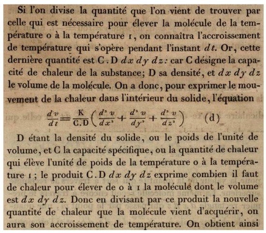
Figure 7.
Fourier heat equation in seminal manuscript of Joseph Fourier [88].
We can also observe that Q is related to the mean, and K to the variance of U:
We observe that the entropy is unchanged, and is changed but with linear dependence to , with the consequence that Fisher Souriau metric is invariant:
We have observed that the concept of “heat capacity” is important in the Souriau model because it gives a geometric meaning to its definition. The notion of “heat capacity” has been generalized by Pierre Duhem in his general equations of thermodynamics.
Souriau [34] proposed to define a thermometer (θερμός) device principle that could measure this geometric temperature using “relative ideal gas thermometer” based on a theory of dynamical group thermometry and has also recovered the (geometric) Laplace barometric law
5. Euler-Poincaré Equations and Variational Principle of Souriau Lie Group Thermodynamics
When a Lie algebra acts locally transitively on the configuration space of a Lagrangian mechanical system, Henri Poincaré proved that the Euler-Lagrange equations are equivalent to a new system of differential equations defined on the product of the configuration space with the Lie algebra. Marle has written about the Euler-Poincaré equations [104], under an intrinsic form, without any reference to a particular system of local coordinates, proving that they can be conveniently expressed in terms of the Legendre and moment maps of the lift to the cotangent bundle of the Lie algebra action on the configuration space. The Lagrangian is a smooth real valued function defined on the tangent bundle . To each parameterized continuous, piecewise smooth curve , defined on a closed interval , with values in , one associates the value at of the action integral:
The partial differential of the function with respect to its second variable , which plays an important part in the Euler-Poincaré equation, can be expressed in terms of the moment and Legendre maps: with the moment map, the canonical projection on the second factor, the Legendre transform, with:
The Euler-Poincaré equation can therefore be written under the form:
with
Following the remark made by Poincaré at the end of his note [105], the most interesting case is when the map only depends on its second variable . The Euler-Poincaré equation becomes:
We can use analogy of structure when the convex Gibbs ensemble is homogeneous [106]. We can then apply Euler-Poincaré equation for Lie group thermodynamics. Considering Clairaut’s equation:
with , , a Souriau-Euler-Poincaré equation can be elaborated for Souriau Lie group thermodynamics:
or
The first equation, the Euler-Poincaré equation is a reduction of Euler-Lagrange equations using symmetries and especially the fact that a group is acting homogeneously on the symplectic manifold:
Back to Koszul model of information geometry, we can then deduce an equivalent of the Euler-Poincaré equation for statistical models
We can use this Euler-Poincaré equation to deduce an associated equation on entropy: that reduces to
due to .
With these new equation of thermodynamics and , we can observe that the new important notion is related to co-adjoint orbits, that are associated to a symplectic manifold by Souriau with KKS 2-form.
We will then define the Poincaré-Cartan integral invariant for Lie group thermodynamics. Classically in mechanics, the Pfaffian form is related to Poincaré-Cartan integral invariant [107]. Dedecker has observed, based on the relation [108]:
that the property that among all forms the form is the only one satisfying , is a particular case of more general Lepage congruence.
Analogies between geometric mechanics and geometric Lie group thermodynamics, provides the following similarities of structures:
We can then consider a similar Poincaré-Cartan-Souriau Pfaffian form:
This analogy provides an associated Poincaré-Cartan-Souriau integral invariant. Poincaré-Cartan integral invariant is given for Souriau thermodynamics by:
We can then deduce an Euler-Poincaré-Souriau variational principle for thermodynamics: The variational principle holds on , for variations , where is an arbitrary path that vanishes at the endpoints, :
6. Souriau Affine Representation of Lie Group and Lie Algebra and Comparison with the Koszul Affine Representation
This affine representation of Lie group/algebra used by Souriau has been intensively studied by Marle [7,100,109,110]. Souriau called the mechanics deduced from this model, “affine mechanics”. We will explain affine representations and associated notions as cocycles, Souriau moment map and cocycles, equivariance of Souriau moment map, action of Lie group on a symplectic manifold and dual spaces of finite-dimensional Lie algebras. We have observed that these tools have been developed in parallel by Jean-Louis Koszul. We will establish close links and synthetize the comparisons in a table of both approaches.
6.1. Affine Representations and Cocycles
Souriau model of Lie group thermodynamics is linked with affine representation of Lie group and Lie algebra. We will give in the following main elements of this affine representation.
Let G be a Lie group and E a finite-dimensional vector space. A map can always be written as:
where the maps and are determined by A. The map A is an affine representation of G in E.
The map is a one-cocycle of G with values in E, for the linear representation R; it means that is a smooth map which satisfies, for all :
The linear representation R is called the linear part of the affine representation A, and is called the one-cocycle of associated to the affine representation A. A one-coboundary of with values in E, for the linear representation R, is a map which can be expressed as:
where c is a fixed element in E and then there exist an element such that, for all and :
Let be a Lie algebra and E a finite-dimensional vector space. A linear map always can be written as:
where the linear maps and are determined by a. The map a is an affine representation of G in E. The linear map is a one-cocycle of G with values in E, for the linear representation r; it means that satisfies, for all :
is called the one-cocycle of associated to the affine representation a. A one-coboundary of with values in E, for the linear representation r, is a linear map which can be expressed as: where c is a fixed element in E., and then there exist an element such that, for all and :
Let be an affine representation of a Lie group in a finite-dimensional vector space E, and be the Lie algebra of . Let and be, respectively, the linear part and the associated cocycle of the affine representation A. Let be the affine representation of the Lie algebra associated to the affine representation of the Lie group . The linear part of a is the linear representation associated to the linear representation , and the associated cocycle is related to the one-cocycle by:
This is deduced from:
Let be a connected and simply connected Lie group, be a linear representation of in a finite-dimensional vector space E, and be the associated linear representation of its Lie algebra . For any one-cocycle of the Lie algebra for the linear representation r, there exists a unique one-cocycle of the Lie group for the linear representation R such that:
in other words, which has as associated Lie algebra one-cocycle. The Lie group one-cocycle is a Lie group one-coboundary if and only if the Lie algebra one-cocycle is a Lie algebra one-coboundary.
which proves that if it exists, the Lie group one-cocycle such that is unique.
6.2. Souriau Moment Map and Cocycles
Souriau first introduced the moment map in his book. We will give the link with previous cocycles of affine representation.
There exist linear application from to differential function on :
We can then associate a differentiable application , called moment(um) map for the Hamiltonian Lie group action :
Let moment map, for each , we associate a smooth function defined by:
It is a Casimir of the Poisson algebra , that satisfies:
When the Poisson manifold is a connected symplectic manifold, the function is constant on M and the map:
is a skew-symmetric bilinear form, and is called the symplectic Cocycle of Lie algebra associated to the moment map .
Let be the map such that for all:
The map is therefore the one-cocycle of the Lie algebra with values in for the coadjoint representation of associated to the affine action of on its dual:
Let be a Lie group whose Lie algebra is . The skew-symmetric bilinear form on can be extended into a closed differential two-form on , since the identity on means that its exterior differential vanishes. In other words, is a 2-cocycle for the restriction of the de Rham cohomology of to left (or right) invariant differential forms.
6.3. Equivariance of Souriau Moment Map
There exists a unique affine action such that the linear part is a coadjoint representation:
with and that induce equivariance of moment .
6.4. Action of Lie Group on a Symplectic Manifold
Let be an action of Lie group G on differentiable manifold M, the fundamental field associated to an element of Lie algebra of group G is the vectors field on M:
is Hamiltonian on a symplectic manifold , if is symplectic and if for all , the fundamental field is globally Hamiltonian.
There is a unique action a of the Lie group on the dual of its Lie algebra for which the moment map J is equivariant, that means satisfies for each
is called cocycle associated to the differential of 1-cocyle associated to J at neutral element :
If instead of J we take the moment map , where is constant, the symplectic cocycle is replaced by:
where is one-coboundary of with values in .
Therefore, the cohomology class of the symplectic cocycle only depends on the Hamiltonian action , not on the choice of its moment map J. We have also:
This property is used by Jean-Marie Souriau [10] to offer a very nice cohomological interpretation of the total mass of a classical (nonrelativistic) isolated mechanical system. He [10] proves that the space of all possible motions of the system is a symplectic manifold on which the Galilean group acts by a Hamiltonian action. The dimension of the symplectic cohomology space of the Galilean group (the quotient of the space of symplectic one-cocycles by the space of symplectic one-coboundaries) is equal to 1. The cohomology class of the symplectic cocycle associated to a moment map of the action of the Galilean group on the space of motions of the system is interpreted as the total mass of the system.
For Hamiltonian actions of a Lie group on a connected symplectic manifold, the equivariance of the moment map with respect to an affine action of the group on the dual of its Lie algebra has been proved by Marle [110]. Marle [110] has also developed the notion of symplectic cocycle and has proved that given a Lie algebra symplectic cocycle, there exists on the associated connected and simply connected Lie group a unique corresponding Lie group symplectic cocycle. Marle [104] has also proved that there exists a two-parameter family of deformations of these actions (the Hamiltonian actions of a Lie group on its cotangent bundle obtained by lifting the actions of the group on itself by translations) into a pair of mutually symplectically orthogonal Hamiltonian actions whose moment maps are equivariant with respect to an affine action involving any given Lie group symplectic cocycle. Marle [104] has also explained why a reduction occurs for Euler-Poncaré equation mainly when the Hamiltonian can be expressed as the moment map composed with a smooth function defined on the dual of the Lie algebra; the Euler-Poincaré equation is then equivalent to the Hamilton equation written on the dual of the Lie algebra.
6.5. Dual Spaces of Finite-Dimensional Lie Algebras
Let be a finite-dimensional Lie algebra, and its dual space. The Lie algebra can be considered as the dual of , that means as the space of linear functions on , and the bracket of the Lie algebra is a composition law on this space of linear functions. This composition law can be extended to the space by setting:
If we apply this formula for Souriau Lie group thermodynamics, and for entropy s(Q) depending on geometric heat Q:
This bracket on defines a Poisson structure on , called its canonical Poisson structure. It implicitly appears in the works of Sophus Lie, and was rediscovered by Alexander Kirillov [111], Bertram Kostant and Jean-Marie Souriau.
The above defined canonical Poisson structure on can be modified by means of a symplectic cocycle by defining the new bracket:
with a symplectic cocycle of the Lie algebra being a skew-symmetric bilinear map which satisfies:
This Poisson structure is called the modified canonical Poisson structure by means of the symplectic cocycle . The symplectic leaves of equipped with this Poisson structure are the orbits of an affine action whose linear part is the coadjoint action, with an additional term determined by .
6.6. Koszul Affine Representation of Lie Group and Lie Algebra
Previously, we have developed Souriau’s works on the affine representation of a Lie group used to elaborate the Lie group thermodynamics. We will study here another approach of affine representation of Lie group and Lie algebra introduced by Jean-Louis Koszul. We consolidate the link of Jean-Louis Koszul work with Souriau model. This model uses an affine representation of a Lie group and of a Lie algebra in a finite-dimensional vector space, seen as special examples of actions.
Since the work of Henri Poincare and Elie Cartan, the theory of differential forms has become an essential instrument of modern differential geometry [112,113,114,115] used by Jean-Marie Souriau for identifying the space of motions as a symplectic manifold. However, as said by Paulette Libermann [116], except Henri Poincaré who wrote shortly before his death a report on the work of Elie Cartan during his application for the Sorbonne University, the French mathematicians did not see the importance of Cartan’s breakthroughs. Souriau followed lectures of Elie Cartan in 1945. The second student of Elie Cartan was Jean-Louis Koszul. Koszul introduced the concepts of affine spaces, affine transformations and affine representations [117,118,119,120,121,122,123,124]. More especially, we are interested by Koszul’s definition for affine representations of Lie groups and Lie algebras. Koszul studied symmetric homogeneous spaces and defined relation between invariant flat affine connections to affine representations of Lie algebras, and characterized invariant Hessian metrics by affine representations of Lie algebras [117,118,119,120,121,122,123,124]. Koszul provided correspondence between symmetric homogeneous spaces with invariant Hessian structures by using affine representations of Lie algebras, and proved that a simply connected symmetric homogeneous space with invariant Hessian structure is a direct product of a Euclidean space and a homogeneous self-dual regular convex cone [117,118,119,120,121,122,123,124]. Let G be a connected Lie group and let G/K be a homogeneous space on which G acts effectively, Koszul gave a bijective correspondence between the set of G-invariant flat connections on G/K and the set of a certain class of affine representations of the Lie algebra of G [117,118,119,120,121,122,123,124]. The main theorem of Koszul is: let G/K be a homogeneous space of a connected Lie group G and let and be the Lie algebras of G and K, assuming that G/K is endowed with a G-invariant flat connection, then admits an affine representation (f,q) on the vector space E. Conversely, suppose that G is simply connected and that is endowed with an affine representation, then G/K admits a G-invariant flat connection.
Koszul has proved the following [117,118,119,120,121,122,123,124]. Let be a convex domain in containing no complete straight lines, and an associated convex cone . Then there exists an affine embedding:
If we consider the group of homomorphism of into given by:
and associated affine representation of Lie algebra:
with the group of all affine transformations of . We have and the pair of the homomorphism and the map is equivariant.
A Hessian structure (D, g) on a homogeneous space G/K is said to be an invariant Hessian structure if both D and g are G-invariant. A homogeneous space G/K with an invariant Hessian structure (D, g) is called a homogeneous Hessian manifold and is denoted by (G/K, D, g). Another result of Koszul is that a homogeneous self-dual regular convex cone is characterized as a simply connected symmetric homogeneous space admitting an invariant Hessian structure that is defined by the positive definite second Koszul form (we have identified in a previous paper that this second Koszul form is related to the Fisher metric). In parallel, Vinberg [125,126] gave a realization of a homogeneous regular convex domain as a real Siegel domain. Koszul has observed that regular convex cones admit canonical Hessian structures, improving some results of Pyateckii-Shapiro that studied realizations of homogeneous bounded domains by considering Siegel domains in connection with automorphic forms. Koszul defined a characteristic function of a regular convex cone , and showed that is a Hessian metric on invariant under affine automorphisms of . If is a homogeneous self dual cone, then the gradient mapping is a symmetry with respect to the canonical Hessian metric, and is a symmetric homogeneous Riemannian manifold. More information on Koszul Hessian geometry can be found in [127,128,129,130,131,132,133,134,135,136].
We will now focus our attention to Koszul affine representation of Lie group/algebra. Let a connex Lie group and a real or complex vector space of finite dimension, Koszul has introduced an affine representation of in such that [117,118,119,120,121,122,123,124]:
is an affine transformation. We set the set of all affine transformations of a vector space , a Lie group called affine transformation group of . The set of all regular linear transformations of , a subgroup of .
We define a linear representation from to :
and an application from to :
Then we have :
deduced from .
On the contrary, if an application from to and a linear representation from to verify previous equation, then we can define an affine representation of in , written :
The condition is equivalent to requiring the following mapping to be an homomorphism:
We write the linear representation of Lie algebra of , defined by and the restriction to of the differential to ( and the differential of and respectively), Koszul has proved that:
where the set of all linear endomorphisms of , the Lie algebra of .
Using the computation,
We can obtain:
where is the unit element in . Since is the identity mapping and , we have the equality: .
A pair of a linear representation of a Lie algebra on and a linear mapping from to is an affine representation of on , if it satisfies .
Conversely, if we assume that admits an affine representation on , using an affine coordinate system on , we can express an affine mapping by an matrix representation:
where is a matrix and is a row vector.
is an injective Lie algebra homomorphism from in the Lie algebra of all matrices, :
If we denote , we write the linear Lie subgroup of generated by . An element of is expressed by:
Let be the orbit of through the origin , then where .
Example.
Let be a convex domain in containing no complete straight lines, we define a convex cone in by . Then there exists an affine embedding:
If we consider the group of homomorphism of into given by:
with the group of all affine transformations of . We have and the pair of the homomorphism and the map is equivariant:
6.7. Comparison of Koszul and Souriau Affine Representation of Lie Group and Lie Algebra
We will compare, in the following Table 1, affine representation of Lie group and Lie algebra from Souriau and Koszul approaches:

Table 1.
Table comparing Souriau and Koszul affine representation of Lie group and Lie algebra.
6.8. Additional Elements on Koszul Affine Representation of Lie Group and Lie Algebra
Let be a local coordinate system on M, the Christoffel’s symbols of the connection are defined by:
The torsion tensor T of D is given by:
The curvature tensor R of D is given by:
The Ricci tensor Ric of D is given by:
In the following, we will consider a homogeneous space G/K endowed with a G-invariant flat connection D (homogeneous flat manifold) written (G/K, D). Koszul has proved a bijective correspondence between the set of G-invariant flat connections on G/K and the set of affine representations of the Lie algebra of G. Let (G, K) be the pair of connected Lie group and its closed subgroup . Let the Lie algebra of and be the Lie subalgebra of corresponding to . is defined as the vector field on induced by the 1-parameter group of transformation . We denote , with the Lie derivative.
Let be the tangent space of at and let consider, the following values at :
where (where is a locally flat linear connection: its torsion and curvature tensors vanish identically), then:
where , and an affine representation of the Lie algebra :
The 1-parameter transformation group generated by is an affine transformation group of V, with linear parts given by and translation vector parts:
These relations are proved by using:
based on the property that the connection D is locally flat and there is local coordinate systems on M such that with a vanishing torsion and curvature:
deduced from the fact the a locally flat linear connection (vanishing of torsion and curvature).
Let be an invariant volume element on in an affine local coordinate system in a neighborhood of :
We can write and develop the Lie derivative of the volume element :
Since the volume element is invariant by G:
By using , we have:
But as D is locally flat and is an infinitesimal affine transformation with respect to D:
The Koszul form and canonical bilinear form are given by:
Then, .
By using , we can obtain:
By using , we can develop:
As and :
If we use that , then we obtain:
To synthetize the result proved by Jean-Louis Koszul, if and are the values of and at , then:
Jean-Louis Koszul has also proved that the inner product on V, given by the Riemannian metric , satisfies the following conditions:
To make the link with Souriau model of thermodynamics, the first Koszul form will play the role of the geometric heat and the second koszul form will be the equivalent of Souriau-Fisher metric that is G-invariant.
Koszul theory is wider and integrates “information geometry” in its corpus. Koszul [117,118,119,120,121,122,123,124] has proved general results, for example: on a complex homogeneous space, an invariant volume defines with the complex structure, an invariant Hermitian form. If this space is a bounded domain, then this hermitian form is positive definite and coincides with the classical Bergman metric of this domain. During his stay at Institute for Advanced Study in Princeton, Koszul [117,118,119,120,121,122,123,124] has also demonstrated the reciprocal for a class of complex homogeneous spaces, defined by open orbits of complex affine transformation groups. Koszul and Vey [137,138] have also developed extended results with the following theorem for connected hessian manifolds:
Theorem 3 (Koszul-Vey Theorem).
Let be a connected hessian manifold with hessian metric . Suppose that M admits a closed 1-form such that and there exists a group of affine automorphisms of preserving :
- If is quasi-compact, then the universal covering manifold of M is affinely isomorphic to a convex domain of an affine space not containing any full straight line.
- If is compact, then is a sharp convex cone.
On this basis, Koszul has given a Lie group construction of a homogeneous cone that has been developed and applied in information geometry by Shima and Boyom in the framework of Hessian geometry. The results of Koszul are also fundamental in the framework of Souriau thermodynamics.
7. Souriau Lie Group Model and Koszul Hessian Geometry Applied in the Context of Information Geometry for Multivariate Gaussian Densities
We will enlighten Souriau model with Koszul hessian geometry applied in information geometry [117,118,119,120,121,122,123,124], recently studied in [3,9,139]. We have previously shown that information geometry could be founded on the notion of Koszul-Vinberg characteristic function where Ω is a convex cone and Ω∗ the dual cone with respect to Cartan-Killing inner product invariant by automorphisms of Ω, with the Killing form and the Cartan involution. We can develop the Koszul characteristic function:
This characteristic function is at the cornerstone of modern concept of information geometry, defining Koszul density by solution of maximum Koszul-Shannon entropy [140]:
This last relation is a Legendre transform between the logarithm of characteristic function and the entropy:
The inversion is given by the Legendre transform based on the property that the Koszul-Shannon entropy is given by the Legendre transform of minus the logarithm of the characteristic function:
We can observe the fundamental property that , and also as observed by Maurice Fréchet that “distinguished functions” (densities with estimator reaching the Fréchet-Darmois bound) are solutions of the Alexis Clairaut equation introduced by Clairaut in 1734 [141], as illustrated in Figure 8:
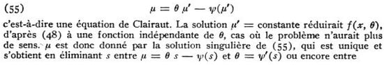
Figure 8.
Clairaut-Legendre equation introduced by Maurice Fréchet in his 1943 paper [141].
Details of Fréchet elaboration for this Clairaut(-Legendre) equation for “distinguished function” is given in Appendix A, and other elements are available on Fréchet’s papers [141,142,143,144].
In this structure, the Fisher metric makes appear naturally a Koszul hessian geometry [145,146], if we observe that
Then we can recover the relation with Fisher metric:
with Crouzeix relation established in 1977 [147,148], giving the dual metric, in dual space, where entropy and (minus) logarithm of characteristic function, , are dual potential functions.
The first metric of information geometry [149,150], the Fisher metric is given by the hessian of the characteristic function logarithm:
The second metric of information geometry is given by hessian of the Shannon entropy:
Both metrics will provide the same distance:
From the Cartan inner product, we can generate logarithm of the Koszul characteristic function, and its Legendre transform to define Koszul entropy, Koszul density and Koszul metric, as explained in the following Figure 9:
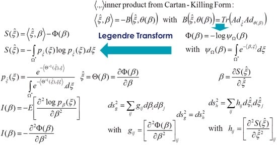
Figure 9.
Generation of Koszul elements from Cartan inner product.
This information geometry has been intensively studied for structured matrices [151,152,153,154,155,156,157,158,159,160,161,162,163,164,165,166] and in statistics [167] and is linked to the seminal work of Siegel [168] on symmetric bounded domains.
We can apply this Koszul geometry framework for cones of symmetric positive definite matrices. Let the inner product given by Cartan-Killing form, be the set of symmetric positive definite matrices is an open convex cone and is self-dual .
We will in the following illustrate information geometry for multivariate Gaussian density [169]:
If we develop:
We can write the density as a Gibbs density:
We can then rewrite density with canonical variables:
The first potential function (free energy/logarithm of characteristic function) is given by:
We verify the relation between the first potential function and moment:
The second potential function (Shannon entropy) is given as a Legendre transform of the first one:
This remark was made by Jean-Souriau in his book [10] as soon as 1969. He has observed, as illustrated in Figure 10 that if we take vector with tensor components , components of will provide moments of the first and second order of the density of probability . He used this change of variable , to compute the logarithm of the characteristic function :
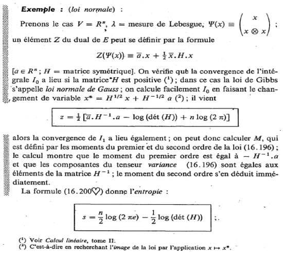
Figure 10.
Introduction of potential function for multivariate Gaussian law in Souriau book [10].
We can finally compute the metric from the matrix :
and from classical expression of the Euler-Lagrange equation:
That is explicitely given by [170]:
We cannot integrate this Euler-Lagrange equation. We will see that Lie group theory will provide new reduced equation, Euler-Poincaré equation, using Souriau theorem.
We make reference to the book of Deza that gives a survey about distance and metric space [171].
The case of Natural Exponential families that are invariant by an affine group has been studied by Casalis (in 1999 paper and in her Ph.D. thesis) [172,173,174,175,176,177,178] and by Letac [179,180,181]. We give the details of Casalis’ development in Appendix C. Barndorff-Nielsen has also studied transformation models for exponential families [182,183,184,185,186]. In this section, we will only consider the case of multivariate Gaussian densities.
8. Affine Group Action for Multivariate Gaussian Densities and Souriau’s Moment Map: Computation of Geodesics by Geodesic Shooting
To more deeply understand Koszul and Souriau Lie group models of information geometry, we will illustrate their tools for multivariate Gaussian densities.
Consider the general linear group consisting of the invertible n × n matrices, that is a topological group acting linearly on by:
The group is a Lie group, is a subgroup of the general affine group , composed of all pairs where and , the group operation given by:
is an open subset of , and may be considered as n2-dimensional differential manifold with the same differentiable structure than . Multiplication and inversion are infinitely often differentiable mappings. Consider the vector space of real n × n matrices and the commutator product:
This is a Lie product making into a Lie algebra. The exponential map is then the mapping defined by:
Restricting to have positive determinant, one obtains the positive general affine group that acts transitively on by:
In case of symmetric positive definite matrices , we can use the Cholesky decomposition:
where is a lower triangular matrix with real and positive diagonal entries, and denotes the transpose of , to define the square root of .
Given a positive semidefinite matrix , according to the spectral theorem, the continuous functional calculus can be applied to obtain a matrix such that is itself positive and . The operator is the unique non-negative square root of .
the class of regular multivariate normal distributions, where is the mean vector and is the (symmetric positive definite) covariance matrix, is invariant under the transitive action of . The induced action of on is then given by:
and
As the isotropy group of is equal to , we can observe that:
is an open subset of the vector space and is a differentiable manifold, where the tangent space at any point may be identified with .
The Fisher information defines a metric given to a Riemannian manifold structure. The inner product of two tangent vectors , at the point is given by:
Niels Christian Bang Jesperson has proved that the transformation model on with parameter set are exactly those of the form where is the Lebesque measure, where and is a continuous function with . Distributions with densities of this form are called elliptic distributions.
To improve understanding of tools, we will consider as a sub-group of affine group, that could be defined by a matrix Lie group , that acts for multivariate Gaussian laws, as illustrated in Figure 11:
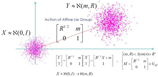
Figure 11.
Affine Lie group action for multivariate Gaussian law.
We can verify that M is a Lie group with classical properties, that product of M preserves the structure, the associativity, the non-commutativity, and the existence of neutral element:
We can also observe that the inverse preserves the structure:
To this Lie group we can associate a Lie algebra whose underlying vector space is the tangent space of the Lie group at the identity element and which completely captures the local structure of the group. This Lie group acts smoothly on the manifold, and acts on the vector fields. Any tangent vector at the identity of a Lie group can be extended to a left (respectively right) invariant vector field by left (respectively right) translating the tangent vector to other points of the manifold. This identifies the tangent space at the identity with the space of left invariant vector fields, and therefore makes the tangent space at the identity into a Lie algebra, called the Lie algebra of G.
Considering the curve and its derivative :
We can consider the curve with the point moved at the identity element on the left or on the right. Then, the tangent plan at identity element provides the Lie algebra:
Lie algebra on the right and on the left is the defined by:
We can then observe the velocities in two different ways, either by placing in a fixed outside frame, either by putting in place of the element in the process of moving by placing in the reference frame of the element.
In the following, we will complete the global view by the operators which will allow to link algebra (from the left or the right) between them and also connect to their dual. We will first consider the automorphisms, the action by conjugation of the Lie group on itself that allows this operator to carry a member of the group.
If now we consider a curve N(t) curve on the manifold via the identity at t = 0. Its image by the previous operator will be then curve passing through identity element at t = 0. As is an element of the Lie algebra and its image by previous conjugation operator is called the Adjoint operator:
We can then compute the Adjoint operator for the previous Lie group:
We recall that the Lie algebra has been defined as the tangent space at the identity of a Lie group. We will then introduce a Lie bracket , the expression of the operator associated with the combined action of the Lie algebra on itself, called an adjoint operator. The adjoint operator represents the action by conjugation of the Lie algebra on itself and is defined by:
We can then compute this operator for our use case:
To study the geodesic trajectories of the group, we consider the Lagrangian from the total kinetic energy (a quadratic form on speeds). It may therefore in particular be written in the left algebra “left”, with the scalar product associated with the metric.
If we consider as scalar product:
and left algebra:
we obtain for the total kinetic energy
We will then introduce the coadjoint operator that will enable us to work on the elements of the dual algebra of the Lie algebra defined above. Like algebra, which is physically the space of instantaneous speeds, the dual algebra is the space of moments. For the dual of left algebra, the moment is given by:
Where is the kinetic energy of the system and is currently associated with is an element of the left algebra. The moment space is the dual algebra, denoted , associated with the Lie algebra . This value is deduced from the computation:
Then the moment map is given by:
We can observe that the application that turns left algebra into dual algebra is the identity application but, physically, the first are moments and the seconds are instantaneous speeds.
We can also define the moment associated to the right algebra by:
But as , we can deduce that:
Then, the operator that transform the right algebra to its dual algebra is given by:
There is an operator to change the view of algebra. Therefore, there is an operator that did the same to the dual algebra. This is called the co-adjoint operator and it is the conjugate action of the Lie group on its dual algebra:
We can then develop this expression for our use in the case of an affine sup-group. We find:
and we can also observe that:
Similarly there exists the following relation between the left and the right algebras:
As we have defined a commutator on the Lie algebra, it is possible to define one on its dual algebra. This commutator on the dual algebra can also be defined using the operator expressing the combined action of the algebra of its dual algebra. This operator is called the co-adjoint operator:
We can develop this co-adjoint operator on its dual algebra for our use-case:
This co-adjoint operator will give the Euler-Poincaré equation. While the Euler-Lagrange equations is defined on the tangent bundle (union of the tangent spaces at each point) of the manifold and give the geodesics, the Euler-Poincaré equation gives a differential system on the dual Lie algebra of the group associated with the manifold.
We can also complete these maps by using additional ones. First, the moment associated with in tangent space of at and also two other moments map the element of the dual algebra in dual tangent space, respectively on the left and on the right:
where
From these relations, we can also observe that:
All these maps could be summarized in the following Figure 12:
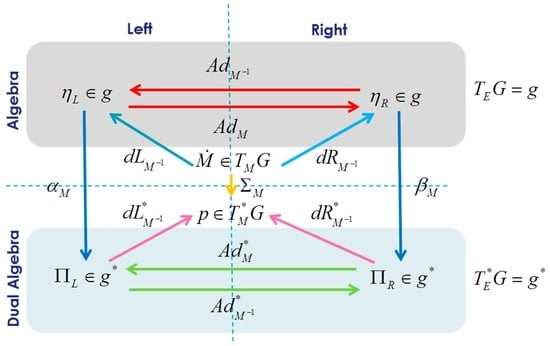
Figure 12.
Maps between algebras.
Heni Poincaré proved that when a Lie algebra acts locally and transitively on the configuration space of a Lagrangian mechanical system, the Euler-Lagrange equations are equivalent to a new system of differential equations defined on the product of the configuration space with the Lie algebra.
If we consider that the following function is stationary for a Lagragian l(.) invariant with respect to the action of a group on the left:
The solution is given by the Euler-Poincaré equation:
If we take for the function l(.), the total kinetic energy , using , then the Euler-Poincaré equation is given by:
The following quantities are conserved:
With this second theorem, it is possible to write the geodesic not from its coordinate system but from the quantity of motion, and in addition to determine explicitly what the conserved quantities along the geodesic are (conservations are related to the symmetries of the variety and hence the invariance of the Lagrangian under the action of the group).
For our use-case, the Euler-Poincaré equation is given by:
If we remark that we have , then the conserved Souriau moment could be given by:
Components of the Souriau moment give the conserved quantities that are the classical elements given by Emmy Noether Theorem (Souriau moment is a geometrization of Emmy Noether Theorem):
From this constant, we can obtain a reduced equation of geodesic:
This is the Euler-Poincaré equation of geodesic. We can observe that we have obtained a reduction of the following Euler-Lagrange equation [27,156,187]: associated to the information geometry metric .
The Fisher information defines a metric turning into a Riemannian manifold. The inner product of two tangent vectors and at the point is given by:
and the geodesic is given by:
We can also observe that the manifold of multivariate Gaussian is homogeneous with respect to positive affine group :
characterized by the action of the group
Since the special orthogonal group is the stabilizer subgroup of , we have the following isomorphism:
We can then restrict the computation of the geodesic from and then we can partially integrate the system of equations:
where are the integration constants.
From this Euler-Poincaré equation, we can compute geodesics by geodesic shooting [188,189,190,191] using classical Eriksen equations [192,193,194,195], by the following change of parameters:
The initial speed of the geodesic is given by . The geodesic shooting is given by the exponential map:
This equation can be interpreted by group theory. could be considered as an element of Lie algebra of the special Lorentz group and more specifically as the element of Cartan Decomposition where is the Lie algebra of a maximal compact sub-group of the group . We know that its exponential map defines a geodesic on Riemannian Symetric space .
This equation can be established by the following developments:
We can then deduce that:
If , then is solution to the geodesic equation previously defined. Since , it suffices to demonstrate that where .
From , using that , we can deduce:
Then , if , that could be verified using relation , by observing that:
We can then compute from two last equations:
As then we can deduce that and then .
To interpret elements of , , opposite points to , and .
Then the geodesic that goes through the origin with initial tangent vector is the curve given by . Then the distance computation is reduced to estimate the initial tangent vector space related by The distance will be then given by the initial tangent vector:
This initial tangent vector will be identified by “Geodesic Shooting”. Let :
Geodesic Shooting is corrected by using Jacobi Field J and parallel transport: solution to with R the Riemann Curvarture tensor.
We consider a geodesic between and with an initial tangent vector , and we suppose that is perturbated by , to . The variation of the final point can be determined thanks to the Jacobi field with and . In term of the exponential map, this could be written:
This could be illustrated in the Figure 13:
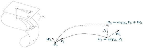
Figure 13.
Geodesic shooting principle.
We give some illustration, in Figure 14, of geodesic shooting to compute the distance between multivariate Gaussian density for the case n = 2:
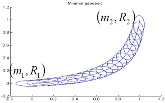
Figure 14.
GeodesicsShooting between two multivariate Gaussian in case n = 2.
9. Souriau Riemannian Metric for Multivariate Gaussian Densities
To illustrate the Souriau-Fisher metric, we will consider the family of multivariate Gaussian densities and will develop some elements that we have previously developed purely theoretically.
For the families of multivariate Gaussian densities, that we have identified as homogeneous manifold with the associated sub-group of the affine group , we have seen that if we consider them as elements of exponential families, we can write (element of the dual Lie algebra) that play the role of geometric heat in Souriau Lie group thermodynamics, and the geometric (Planck) temperature.
These elements are homeomorphic to the matrix elements in matrix Lie algebra and dual Lie algebra:
If we consider , then we can compute the co-adjoint operator:
We can also compute the adjoint operator:
We can rewrite with the following identification:
We have then to develop , that is to say after action of the group on the Lie algebra for , given by . By analogy of structure between and , we can write:
We have then to identify the cocycle from where:
The cocycle is then given by:
From , we can compute cocycle in Lie algebra
used to define the tensor:
In this second part, we will compute the Souriau-Fisher metric given by:
with
where
With the inner product given by
We can then compute:
The Souriau-Fisher metric is defined in Lie algebra where:
and
Another approach to develop the Souriau-Fisher metric is to compute the tensor from the moment map :
We can then write the Souriau-Fisher metric as:
Where the associated differentiable application , called moment map is:
This moment map could be identified with the operator that transforms the right algebra to an element of its dual algebra given by:
10. Conclusions
In this paper, we have developed a Souriau model of Lie group thermodynamics that recovers the symmetry broken by lack of covariance of Gibbs density in classical statistical mechanics with respect to dynamic groups action in physics (Galileo and Poincaré groups, sub-group of affine group). The ontological model of Souriau gives geometric status to (Planck) temperature (element of Lie alebra), heat (element of dual Lie algebra) and entropy. Souriau said in one of his papers [30] on this new “Lie group thermodynamics” that “these formulas are universal, in that they do not involve the symplectic manifold, but only group G, the symplectic cocycle. Perhaps this Lie group thermodynamics could be of interest for mathematics”.
For this new covariant thermodynamics, the fundamental notion is the coadjoint orbit that is linked to positive definite KKS (Kostant–Kirillov–Souriau) 2-form [196]:
that is the Kähler-form of a G-invariant kähler structure compatible with the canonical complex structure of M, and determines a canonical symplectic structure on M. When the cocycle is equal to zero, the KKS and Souriau-Fisher metric are equal. This 2-form introduced by Jean-Marie Souriau is linked to the coadjoint action and the coadjoint orbits of the group on its moment space. Souriau provided a classification of the homogeneous symplectic manifolds with this moment map. The coadjoint representation of a Lie group G is the dual of the adjoint representation. If denotes the Lie algebra of G, the corresponding action of G on , the dual space to , is called the coadjoint action. Souriau proved based on the moment map that a symplectic manifold is always a coadjoint orbit, affine of its group of Hamiltonian transformations, deducing that coadjoint orbits are the universal models of symplectic manifolds: a symplectic manifold homogeneous under the action of a Lie group, is isomorphic, up to a covering, to a coadjoint orbit. So the link between Souriau-Fisher metric and KKS 2-form will provide a symplectic structure and foundation to information manifolds. For Souriau thermodynamics, the Souriau-Fisher metric is the canonical structure linked to KKS 2-form, modified by the cocycle (its symplectic leaves are the orbits of the affine action that makes equivariant the moment map). This last property allows us to determine all homogeneous spaces of a Lie group admitting an invariant symplectic structure by the action of this group: for example, there are the orbits of the coadjoint representation of this group or of a central extension of this group (the central extension allowing suppressing the cocycle). For affine coadjoint orbits, we make reference to Alice Tumpach Ph.D. [197,198,199] who has developed previous works of Neeb [200], Biquard and Gauduchon [201,202,203,204].
Other promising domains of research are theory of generating maps [205,206,207,208] and the link with Poisson geometry through affine Poisson group. As observed by Pierre Dazord [209] in his paper “Groupe de Poisson Affines”, the extension of a Poisson group to an affine Poisson group due to Drinfel’d [210] includes the affine structures of Souriau on dual Lie algebra. For an affine Poisson group, its universal covering could be identified to a vector space with an associated affine structure. If this vector space is an abelian affine Poisson group, we can find the affine structure of Souriau. For the abelian group (R3,+), affine Poisson groups are the affine structures of Souriau.
Souriau model of Lie group thermodynamics could be a promising way to achieve René Thom’s dream to replace thermodynamics by geometry [211,212], and could be extended to the second order extension of the Gibbs state [213,214].
We could explore the links between “stochastic mechanics” (mécanique alétoire) developed by Jean-Michel Bismut based on Malliavin Calculus (stochastic calculus of variations) and Souriau “Lie group thermodynamics”, especially to extend covariant Souriau Gibbs density on the stochastic symplectic manifold (e.g., to model centrifuge with random vibrating axe and the Gibbs density).
We have seen that Souriau has replaced classical Maximum Entropy approach by replacing Lagrange parameters by only one geometric “temperature vector” as element of Lie algebra. In parallel, as refered in [15], Ingarden has introduced [213,214] second and higher order temperature of the Gibbs state that could be extended to Souriau theory of thermodynamics. Ingarden higher order temperatures could be defined in the case when no variational is considered, but when a probability distribution depending on more than one parameter. It has been observed that Ingarden can fail if the following assumptions are not fulfilled: the number of components of the sum goes to infinity and the components of the sum are stochastically independent. Gibbs hypothesis can also fail if stochastic interactions with the environment are not sufficiently weak. In all these cases, we never observe absolute thermal equilibrium of Gibbs type but only flows or turbulence. Nonequilibrium thermodynamics could be indirectly addressed by means of the concept of high order temperatures. Momentum should be replaced by higher order moments given by the relation defined by extended Massieu characteristic function . Entropy is defined by Legendre transform of this Massieu characteristic function where . We are able also to define high order thermal capacities given by . The Gibbs density could be then extended with respect to high order temperatures by .
We also have to make reference to the works of Streater [16], Nencka [215] and Burdet [216]. Nencka and Streater [215], for certain unitary representations of a Lie algebra , define the statistical manifold of states as the convex cone of for which the partition function is finite. The Hessian of defines a Riemannian metric g on dual Lie algebra . They observe that foliates into the union of coadjoint orbits, each of which can be given a complex Kostant structure (that of Kostant).
To conclude, we will make reference to Alain Berthoz [217] at College de France who has studied brain coding of movement. The most recent studies on this topic, by Alexandre Afgoustidis Ph.D. [218] “Invariant Harmonic Analysis and Geometry in the Workings of the Brain” supervised by Daniel Bennequin, Afgoustidis [218] consolidate the idea that brain vestibular channels and otolithes code Lie algebra of the homogeneous Galileo group as illustrated in the following Figure 15.
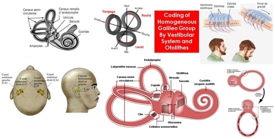
Figure 15.
Coding of homogeneous Galileo algebra by vestibular system and otolithes.
Souriau gave the same ideas in this direction regarding how the brain could code invariants [219]:
Lorsque il y un tremblement de terre, nous assistons à la mort de l’Espace. … Nous vivons avec nos habitudes que nous pensons universelles. … La neuroscience s’occupe rarement de la géométrie … Pour les singes qui vivent dans les arbres, certaines propriétés du groupe d’Euclide sont mieux câblées dans leurs cerveaux (When there is an earthquake, we are witnessing the death of Space … We live with our habits that we think are universal.... Neuroscience rarely is interested in geometry … For the monkeys that live in trees, some properties of the Euclid group are better coded in their brains).
Souriau added anecdotes from a discussion with a student of Bohr that [220]:
L’élève demanda à Bohr qu’il ne comprenait pas le principe de correspondance. Bohr lui demanda de s’assoir et il tourna autour de lui. Bohr lui dit tu dois commencer à avoir mal au cœur, c’est que tu commences à comprendre ce qu’est le principe de correspondance (The student said to Bohr that he did not understand the principle of correspondence. Bohr asked him to sit and he turned around. Bohr said, you should start to be seasick, it is then that you begin to understand what the correspondence principle is.).
Acknowledgments
I would like to thank Charles-Michel Marle and Gery de Saxcé for the fruitful discussions on Souriau model of statistical physics that help me to understand the fundamental notion of affine representation of Lie group and algebra, moment map and coadjoint orbits. I would also like to thank Michel Boyom that introduce me to Jean-Louis Koszul works on affine representation of Lie group and Lie algebra.
Si on ajoute que la critique qui accoutume l’esprit, surtout en matière de faits, à recevoir de simples probabilités pour des preuves, est, par cet endroit, moins propre à le former, que ne le doit être la géométrie qui lui fait contracter l’habitude de n’acquiescer qu’à l’évidence; nous répliquerons qu’à la rigueur on pourrait conclure de cette différence même, que la critique donne, au contraire, plus d’exercice à l’esprit que la géométrie: parce que l’évidence, qui est une et absolue, le fixe au premier aspect sans lui laisser ni la liberté de douter, ni le mérite de choisir; au lieu que les probabilités étant susceptibles du plus et du moins, il faut, pour se mettre en état de prendre un parti, les comparer ensemble, les discuter et les peser. Un genre d’étude qui rompt, pour ainsi dire, l’esprit à cette opération, est certainement d’un usage plus étendu que celui où tout est soumis à l’évidence; parce que les occasions de se déterminer sur des vraisemblances ou probabilités, sont plus fréquentes que celles qui exigent qu’on procède par démonstrations: pourquoi ne dirions –nous pas que souvent elles tiennent aussi à des objets beaucoup plus importants?—Joseph de Maistre in L’Espit de Finesse [221]
Le cadavre qui s’acoutre se méconnait et imaginant l’éternité s’en approrie l’illusion … C’est pourquoi j’abandonnerai ces frusques et jetant le masque de mes jours, je fuirai le temps où, de concert avec les autres, je m’éreinte à me trahir.—Emile Cioran in Précis de decomposition [222]
Conflicts of Interest
The author declares no conflict of interest.
Appendix A. Clairaut(-Legendre) Equation of Maurice Fréchet Associated to “Distinguished Functions” as Fundamental Equation of Information Geometry
Before Rao [223,224], in 1943, Maurice Fréchet [141] wrote a seminal paper introducing what was then called the Cramer-Rao bound. This paper contains in fact much more that this important discovery. In particular, Maurice Fréchet introduces more general notions relative to “distinguished functions”, densities with estimator reaching the bound, defined with a function, solution of Clairaut’s equation. The solutions “envelope of the Clairaut’s equation” are equivalent to standard Legendre transform without convexity constraints but only smoothness assumption. This Fréchet’s analysis can be revisited on the basis of Jean-Louis Koszul’s works as a seminal foundation of “information geometry”.
We will use Maurice Fréchet notations, to consider the estimator:
and the random variable
that are associated to:
The normalizing constraint implies that:
If we consider the derivative if this last expression with respect to , then
Similarly, if we assume that , then , and we obtain by derivation with respect to :
But as and , we immediately deduce that:
From Schwarz inequality, we can develop the following relations:
U being the summation of independent variables, Bienaymé equality could be applied:
From which, Fréchet deduced the bound, rediscovered by Cramer and Rao 2 years later:
Fréchet [141] observed that it is a remarkable inequality where the second member is independent of the choice of the function H defining the “empirical value” T, where the first member can be taken to any empirical value subject to the unique condition regardless is .
The classic condition that the Schwarz inequality becomes an equality helps us to determine when reaches its lower bound .
The previous inequality becomes an equality if there are two numbers and (not random and not both zero ) such that , with being a particular function among eligible such that we have an equality. This equality is rewritten with being a non-random number.
If we use the previous equation, then:
We obtain:
From which we obtain and the form of the associated estimator :
It is therefore deduced that the estimator that reaches the terminal is of the form:
with .
would be one of the eligible functions, if would be independent of . Indeed, if we consider , .
satisfies the equation and inequality shows that it is almost certainly equal to .
So to look for , we should know beforehand .
At this stage, Fréchet [141] looked for “distinguished functions” (“densités distinguées” in French), as any probability density such that the function:
is independent of . The objective of Fréchet is then to determine the minimizing function that reaches the bound. We can deduce from previous relations that:
But as , we can consider as the second derivative of a function such that:
From which we deduce that:
Is an independent quantity of . A distinguished function will be then given by:
With the normalizing constraint .
These two conditions are sufficient. Indeed, reciprocally, let three functions , and that we have, for any
Then the function is distinguished:
The function is reduced to and then is not dependent of .
We have then the following relation:
The relation is valid for any , we can derive prefious equation with respect with :
We can divide by because it does not depend on .
If we derive again with respect to , we will have:
Combining this relation with that of , we can deduce that and as then .
Fréchet emphasizes at this step [141], another way to approach the problem. We can select arbitrarily and and then is determined by:
That could be rewritten:
If we then fixed arbitrarily and and let s an arbitrary variable, the following function will be an explicit positive function given by :
Fréchet obtained finally the function as solution of the equation [141]:
Fréchet noted that this is the Alexis Clairaut equation [141].
The case would reduce the density to a function that would be independent of , and so is given by a singular solution of this Clairaut equation, which is unique and could be computed by eliminating the variable s between:
Or between:
where s is given implicitly by .
Then we know the distinguished function, among functions verifying and such that reaches for each value of , an absolute minimum, equal to .
For the previous equation:
We can rewrite the estimator as:
and compute the associated empirical value:
If we take , we have as :
When is a distinguished function, the empirical value of corresponding to a sample is a root of previous equation in . This equation has a root and only one when X is a distinguished variable. Indeed, as we have:
We can then recover the unique root: .
This function can have an arbitrary form, that is a sum of functions of each only one of the quantities and it is even the arithmetic average of N values of a same auxiliary random variable . The dispersion is given by:
and follows the probability density:
Clairaut Equation and Legendre Transform
We have just observed that Fréchet shows that distinguished functions depend on a function , solution of the Clairaut equation:
Or given by the Legendre transform:
Fréchet also observed that this function could be rewritten:
where s is given implicitly by .
This equation is the fundamental equation of information geometry.
The “Legendre” transform was introduced by Adrien-Marie Legendre in 1787 [225] to solve a minimal surface problem Gaspard Monge in 1784. Using a result of Jean Baptiste Meusnier, a student of Monge, it solves the problem by a change of variable corresponding to the transform which now entitled with his name. Legendre wrote: “I have just arrived by a change of variables that can be useful in other occasions.” About this transformation, Darboux [226] in his book gives an interpretation of Chasles: “This comes after a comment by Mr. Chasles, to substitute its polar reciprocal on the surface compared to a paraboloïd.” The equation of Clairaut was introduced 40 years earlier in 1734 by Alexis Clairaut [225]. Solutions “envelope of the Clairaut equation” are equivalent to the Legendre transform with unconditional convexity, but only under differentiability constraint. Indeed, for a non-convex function, Legendre transformation is not defined where the Hessian of the function is canceled, so that the equation of Clairaut only makes the hypothesis of differentiability. The portion of the strictly convex function g in Clairaut equation y = px − g(p) to the function f giving the envelope solutions by the formula y = f(x) is precisely the Legendre transformation. The approach of Fréchet may be reconsidered in a more general context on the basis of the work of Jean-Louis Koszul.
Appendix B. Balian Gauge Model of Thermodynamics and its Compliance with Souriau Model
Supported by Industial group TOTAL (previously Elf-Aquitaine), Roger Balian has introduced a Gauge theory of thermodynamics [103] and has also developed information geometry in statistical physics and quantum physics [103,227,228,229,230,231,232,233,234,235]. Balian has observed that the entropy (we use Balian notation, contrary with previous section where we use as neg-entropy) can be regarded as an extensive variable , with , n independent quantities, usually extensive and conservative, characterizing the system. The n intensive variables are defined as the partial derivatives:
Balian has introduced a non-vanishing gauge variable , without physical relevance, which multiplies all the intensive variables, defining a new set of variables:
The 2n + 1-dimensional space is thereby extended into a 2n + 2-dimensional thermodynamic space spanned by the variables , where the physical system is associated with a n + 1-dimensional manifold in , parameterized for instance by the coordinates and . A gauge transformation which changes the extra variable while keeping the ratios invariant is not observable, so that a state of the system is represented by any point of a one-dimensional ray lying in , along which the physical variables are fixed. Then, the relation between contact and canonical transformations is a direct outcome of this gauge invariance: the contact structure in n + 1 dimension can be embedded into a symplectic structure in 2n + 2 dimension, with 1-form:
as symplectization, with geometric interpretation in the theory of fiber bundles.
The n + 1-dimensional thermodynamic manifolds are characterized by the vanishing of this form . The 1-form induces then a symplectic structure on :
Any thermodynamic manifold belongs to the set of the so-called Lagrangian manifolds in , which are the integral submanifolds of with maximum dimension (n + 1). Moreover, is gauge invariant, which is implied by . The extensivity of the entropy function is expressed by the Gibbs-Duhem relation , rewritten with previous relation , defining a 2n + 1-dimensional extensivity sheet in , where the thermodynamic manifolds should lie. Considering an infinitesimal canonical transformation, generated by the Hamiltonian , and , the Hamilton’s equations are given by Poisson bracket:
The concavity of the entropy , as function of the extensive variables, expresses the stability of equilibrium states. This property produces constraints on the physical manifolds in the 2n + 2-dimensional space. It entails the existence of a metric structure in the n-dimensional space relying on the quadratic form:
which defines a distance between two neighboring thermodynamic states.
The factor ensures gauge invariance. In a continuous transformation generated by , the metric evolves according to:
We can observe that this gauge theory of thermodynamics is compatible with Souriau Lie groupTthermodynamics, where we have to consider the Souriau vector , transformed in a new vector:
Appendix C. Casalis-Letac Affine Group Invariance for Natural Exponential Families
The characterization of the natural exponential families of Rd which are preserved by a group of affine transformations has been examined by Muriel Casalis in her Ph.D. [173] and her different papers [172,174,175,176,177,178]. Her method has consisted of translating the invariance property of the family into a property concerning the measures which generate it, and to characterize such measures.
Let a vector space of finite size, its dual. duality bracket with . positive Radon measure on , Laplace transform is:
Let transformation defined on :
natural exponential families are given by:
with injective function (domain of means):
the inverse function:
and the Covariance operator:
Measure generetad by a family is then given by:
Let an exponential family of generated by and with automorphisms of and , then the family is an exponential familly of generated by
Definition C1.
An exponential family is invariant by a group (affine group of ), if
(the contrary could be false)
Then Muriel Casalis has established the following theorem:
Theorem C1 (Casalis).
Let an exponential family of and affine group of , then is invariant by if and only:
When is a linear subgroup, is a character of and could be obtained by the help of cohomology of Lie groups.
If we define action of on by:
It can be verified that:
the action a is an inhomogeneous 1-cocycle:
, let the set of all functions from to , called inhomogenesous n-cochains, then we can define the operators by:
Let , with inhomogneous n-cocycles, the quotient:
is the Cohomology group of with value in . We have:
When the Cohomology group then:
Then if is an exponential family invariant by , verifies:
For all compact group, and we can express a:
References and Notes
- Bernard, C. Introduction à l’Étude de la Médecine Expérimentale. Available online: http://classiques.uqac.ca/classiques/bernard_claude/intro_etude_medecine_exp/intro_medecine_exper.pdf (accessed on 17 October 2016).
- Thom, R. Logos et Théorie des Catastrophes; Editions Patiño: Genève, Switzerland, 1988. [Google Scholar]
- Barbaresco, F. Symplectic structure of information geometry: Fisher metric and Euler-Poincaré equation of souriau lie group thermodynamics. In Geometric Science of Information, Second International Conference GSI 2015; Nielsen, F., Barbaresco, F., Eds.; Springer: Berlin/Heidelberg, Germany, 2015; Volume 9389, pp. 529–540. [Google Scholar]
- De Saxcé, G.; Vallée, C. Galilean Mechanics and Thermodynamics of Continua; Wiley-ISTE: London, UK, 2016. [Google Scholar]
- Vallée, C. Relativistic thermodynamics of continua. Int. J. Eng. Sci. 1981, 19, 589–601. [Google Scholar] [CrossRef]
- Vallée, C.; Lerintiu, C. Convex analysis and entropy calculation in statistical mechanics. Proc. A Razmadze Math. Inst. 2005, 137, 111–129. [Google Scholar]
- Marle, C.M. From Tools in Symplectic and Poisson Geometry to J.-M. Souriau’s Theories of Statistical Mechanics and Thermodynamics. Entropy 2016, 18, 370. [Google Scholar] [CrossRef]
- De Saxcé, G. Link between lie group statistical mechanics and thermodynamics of continua. In Special Issue MDPI Entropy “Differential Geometrical Theory of Statistics”; MDPI: Basel, Switzerland, 2016; Volume 18, p. 254. [Google Scholar]
- Barbaresco, F. Koszul information geometry and souriau geometric temperature/capacity of lie group thermodynamics. Entropy 2014, 16, 4521–4565. [Google Scholar] [CrossRef]
- Souriau, J.M. Structure des Systèmes Dynamiques; Editions Jacques Gabay: Paris, France, 1970. (In French) [Google Scholar]
- Souriau, J.M. Structure of Dynamical Systems, volume 149 of Progress in Mathematics. In A Symplectic View of Physics; Birkhäuser: Basel, Switzerland, 1997. [Google Scholar]
- Nielsen, F.; Barbaresco, F. Geometric Science of Information; Springer: Berlin/Heidelberg, Germany, 2015. [Google Scholar]
- Kosmann-Schwarzbach, Y. La géométrie de Poisson, création du XXième siècle. In Siméon-Denis Poisson; Ecole Polytechnique: Paris, France, 2013; pp. 129–172. [Google Scholar]
- Bismut, J.M. Mécanique Aléatoire; Springer: Berlin/Heidelberg, Germany, 1981; Volume 866. [Google Scholar]
- Casas-Vázquez, J.; Jou, D. Temperature in non-equilibrium states: A review of open problems and current proposals. Rep. Prog. Phys. 2003, 66, 1937–2023. [Google Scholar] [CrossRef]
- Streater, R.F. The information manifold for relatively bounded potentials. Tr. Mat. Inst. Steklova 2000, 228, 217–235. [Google Scholar]
- Arnold, V.I. Sur la géométrie différentielle des groupes de Lie de dimension infinie et ses applications à l’hydrodynamique des fluides parfaits. Ann. Inst. Fourier 1966, 16, 319–361. [Google Scholar] [CrossRef]
- Arnold, V.I.; Givental, A.B. Symplectic geometry. In Dynamical Systems IV: Symplectic Geometry and Its Applications, Encyclopaedia of Mathematical Sciences; Arnol’d, V.I., Novikov, S.P., Eds.; Springer: Berlin, Germany, 1990; Volume 4, pp. 1–136. [Google Scholar]
- Marle, C.M.; de Saxcé, G.; Vallée, C. L’oeuvre de Jean-Marie Souriau, Gazette de la SMF, Hommage à Jean-Marie Souriau. 2012; Published by SMF, Paris. [Google Scholar]
- Patrick Iglesias, Itinéraire d’un Mathématicien: Un entretien Avec Jean-Marie Souriau, Le Journal de Maths des Elèves. Available online: http://www.lutecium.fr/jp-petit/science/gal_port/interview_Souriau.pdf (accessed on 27 October 2016). (In French)
- Iglesias, P. Symétries et Moment; Hermann: Paris, France, 2000. [Google Scholar]
- Kosmann-Schwarzbach, Y. Groupes et Symmetries; Ecole Polytechnique: Paris, France, 2006. [Google Scholar]
- Kosmann-Schwarzbach, Y. En homage à Jean-Marie Souriau, quelques souvenirs. Gazette des Mathématiciens 2012, 133, 105–106. [Google Scholar]
- Ghys, E. Actions localement libres du groupe affine. Invent. Math. 1985, 82, 479–526. [Google Scholar] [CrossRef]
- Rais, M. La representation coadjointe du groupe affine. Ann. Inst. Fourier 1978, 28, 207–237. (In French) [Google Scholar] [CrossRef]
- Souriau, J.M. Mécanique des états condensés de la matière. In Proceedings of the 1st International Seminar of Mechanics Federation of Grenoble, Grenoble, France, 19–21 May 1992. (In French)
- Souriau, J.M. Géométrie de l’espace de phases. Commun. Math. Phys. 1966, 374, 1–30. (In French) [Google Scholar]
- Souriau, J.M. Définition covariante des équilibres thermodynamiques. Nuovo Cimento 1966, 1, 203–216. (In French) [Google Scholar]
- Souriau, J.M. Mécanique Statistique, Groupes de Lie et Cosmologie; Colloques Internationaux du CNRS Numéro 237: Paris, France, 1974; pp. 59–113. (In French) [Google Scholar]
- Souriau, J.M. Géométrie Symplectique et Physique Mathématique; Éditions du C.N.R.S.: Paris, France, 1975. (In French) [Google Scholar]
- Souriau, J.M. Thermodynamique Relativiste des Fluides; Centre de Physique Théorique: Marseille, France, 1977. (In French) [Google Scholar]
- Souriau, J.M. Interpretation Géometrique des Etatsquantiques; Springer: Berlin/Heidelberg, Germany, 1977; Volume 570. (In French) [Google Scholar]
- Souriau, J.M. Thermodynamique et géométrie. In Differential Geometrical Methods in Mathematical Physics II; Bleuler, K., Reetz, A., Petry, H.R., Eds.; Springer: Berlin/Heidelberg, Germany, 1978; pp. 369–397. (In French) [Google Scholar]
- Souriau, J.M. Dynamic Systems Structure, Chapters 16–19. Unpublished work. 1980.
- Souriau, J.M.; Iglesias, P. Heat Cold and Geometry. Differential Geometry and Mathematical Physics, Mathematical Physics Studies Volume; Springer: Amsterdam, The Netherlands, 1983; pp. 37–68. [Google Scholar]
- Souriau, J.M. Mécanique classique et géométrie symplectique. CNRS Marseille. Cent. Phys. Théor. Report ref. CPT-84/PE-1695 1984. (In French)
- Souriau, J.M. On Geometric Mechanics. Discret. Cont. Dyn. Syst. J. 2007, 19, 595–607. [Google Scholar] [CrossRef]
- Laplace, P.S. Mémoire sur la probabilité des causes sur les évènements. In Mémoires de Mathématique et de Physique; De l’Imprimerie Royale: Paris, France, 1774. (In French) [Google Scholar]
- Gibbs, J.W. Elementary principles in statistical mechanics. In The Rational Foundation of Thermodynamics; Scribner: New York, NY, USA, 1902. [Google Scholar]
- Ruelle, D.P. Thermodynamic Formalism; Addison-Wesley: New York, NY, USA, 1978. [Google Scholar]
- Ruelle, D.P. Extending the definition of entropy to nonequilibrium steady states. Proc. Natl. Acad. Sci. USA 2003, 100, 3054–3058. [Google Scholar] [CrossRef] [PubMed]
- Jaynes, E.T. Information theory and statistical mechanics. Phys. Rev. 1957, 106, 620–630. [Google Scholar] [CrossRef]
- Jaynes, E.T. Information theory and statistical mechanics II. Phys. Rev. 1957, 108, 171–190. [Google Scholar] [CrossRef]
- Jaynes, E.T. Prior probabilities. IEEE Trans. Syst. Sci. Cybern. 1968, 4, 227–241. [Google Scholar] [CrossRef]
- Jaynes, E.T. The well-posed problem. Found. Phys. 1973, 3, 477–493. [Google Scholar] [CrossRef]
- Jaynes, E.T. Where do we stand on maximum entropy? In The Maximum Entropy Formalism; Levine, R.D., Tribus, M., Eds.; MIT Press: Cambridge, MA, USA, 1979; pp. 15–118. [Google Scholar]
- Jaynes, E.T. The minimum entropy production principle. Annu. Rev. Phys. Chem. 1980, 31, 579–601. [Google Scholar] [CrossRef]
- Jaynes, E.T. On the rationale of maximum entropy methods. IEEE Proc. 1982, 70, 939–952. [Google Scholar] [CrossRef]
- Jaynes, E.T. Papers on Probability, Statistics and Statistical Physics; Reidel: Dordrecht, The Netherlands, 1982. [Google Scholar]
- Ollivier, Y. Aspects de l’entropie en Mathématiques et en Physique (Théorie de l’information, Systèmes Dynamiques, Grandes Déviations, Irréversibilité). Available online: http://www.yann-ollivier.org/entropie/entropie.pdf (accessed on 7 August 2015). (In French)
- Villani, C. (Ir)rréversibilité et Entropie. Available online: http://www.bourbaphy.fr/villani.pdf (accessed on 5 August 2015). (In French)
- Godement, R. Introduction à la Théorie des Groupes de Lie; Springer: Berlin/Heidelberg, Germany, 2004. [Google Scholar]
- Guichardet, A. Cohomologie des Groups Topologiques et des Algèbres de Lie; Cedic/Fernand Nathan: Paris, France, 1980. [Google Scholar]
- Guichardet, A. La method des orbites: Historiques, principes, résultats. In Leçons de Mathématiques D’aujourd’hui; Cassini: Paris, France, 2010; Volume 4, pp. 33–59. [Google Scholar]
- Guichardet, A. Le Problème de Kepler, Histoire et Théorie; Ecole Polytechnique: Paris, France, 2012. [Google Scholar]
- Dubois, J.G.; Dufour, J.P. La théorie des catastrophes. V. Transformées de Legendre et thermodynamique. In Annales de l’IHP Physique Théorique; Institut Henri Poincaré: Paris, France, 1978; Volume 29, pp. 1–50. [Google Scholar]
- Monge, G. Sur le Calcul Intégral des Equations aux Différences Partielles; Mémoires de l’Académie des Sciences: Paris, France, 1784; pp. 118–192. (In French) [Google Scholar]
- Moreau, J.J. Fonctions convexes duales et points proximaux dans un espace hilbertien. C. R. Acad. Sci. 1962, 255, 2897–2899. (In French) [Google Scholar]
- Plastino, A.; Plastino, A.R. On the Universality of thermodynamics’ Legendre transform structure. Phys. Lett. A 1997, 226, 257–263. [Google Scholar] [CrossRef]
- Friedrich, T. Die fisher-information und symplectische strukturen. Math. Nachr. 1991, 153, 273–296. (In German) [Google Scholar] [CrossRef]
- Massieu, F. Sur les Fonctions caractéristiques des divers fluides. C. R. Acad. Sci. 1869, 69, 858–862. (In French) [Google Scholar]
- Massieu, F. Addition au précédent Mémoire sur les Fonctions caractéristiques. C. R. Acad. Sci. 1869, 69, 1057–1061. (In French) [Google Scholar]
- Massieu, F. Exposé des Principes Fondamentaux de la Théorie Mécanique de la Chaleur (note Destinée à Servir D’introduction au Mémoire de L’auteur sur les Fonctions Caractéristiques des Divers Fluides et la Théorie des Vapeurs); Académie des Sciences: Paris, France, 1873; p. 31. (In French) [Google Scholar]
- Massieu, F. Thermodynamique: Mémoire sur les Fonctions Caractéristiques des Divers Fluides et sur la Théorie des Vapeurs; Académie des Sciences: Paris, France, 1876; p. 92. (In French) [Google Scholar]
- Massieu, F. Sur les Intégrales Algébriques des Problèmes de Mécanique. Suivie de Sur le Mode de Propagation des Ondes Planes et la Surface de L’onde Elémentaire dans les Cristaux Biréfringents à Deux Axes. Ph.D. Thesis, Faculté des Sciences de Paris, Paris, France, 1861. [Google Scholar]
- Nivoit, E. Notice sur la vie et les Travaux de M. Massieu, Inspecteur Général des Mines. Available online: http://facultes19.ish-lyon.cnrs.fr/fiche.php?indice=1153 (accessed 27 October).
- Gibbs, J.W. Graphical Methods in the Thermodynamics of Fluids. In The Scientific Papers of J. Willard Gibbs; Dover: New York, NY, USA, 1961. [Google Scholar]
- Brillouin, L. Science and Information Theory; Academic Press: New York, NY, USA, 1956. [Google Scholar]
- Brillouin, L. Maxwell’s demon cannot operate: Information and entropy. J. Appl. Phys. 1951, 22, 334–337. [Google Scholar] [CrossRef]
- Brillouin, L. Physical entropy and information. J. Appl. Phys. 1951, 22, 338–343. [Google Scholar] [CrossRef]
- Brillouin, L. Negentropy principle of information. J. Appl. Phys. 1953, 24, 1152–1163. [Google Scholar] [CrossRef]
- Duhem, P. Sur les équations générales de la thermodynamique. In Annales scientifiques de l’École Normale Supérieure; Ecole Normale Supérieure: Paris, France, 1891; Volume 8, pp. 231–266. (In French) [Google Scholar]
- Duhem, P. Commentaire aux principes de la Thermodynamique—Première partie. J. Math. Appl. 1892, 8, 269–330. (In French) [Google Scholar]
- Duhem, P. Commentaire aux principes de la Thermodynamique—Troisième partie. J. Math. Appl. 1894, 10, 207–286. (In French) [Google Scholar]
- Duhem, P. Les théories de la chaleur. Revue des deux Mondes 1895, 130, 851–868. [Google Scholar]
- Carathéodory, C. Untersuchungen über die Grundlagen der Thermodynamik (Examination of the foundations of thermodynamics). Math. Ann. 1909, 67, 355–386. [Google Scholar] [CrossRef]
- Carnot, S. Réflexions sur la Puissance Motrice du feu; Dover: New York, NY, USA, 1960. [Google Scholar]
- Clausius, R. On the Mechanical Theory of Heat; Browne, W.R., Translator; Macmillan: London, UK, 1879. [Google Scholar]
- Darrigol, O. The Origins of the Entropy Concept. Available online: http://www.bourbaphy.fr/darrigol.pdf (accessed on 5 August 2015). (In French)
- Gromov, M. In a Search for a Structure, Part 1: On Entropy. Available online: http://www.ihes.fr/~gromov/PDF/structre-serch-entropy-july5-2012.pdf (accessed on 6 August 2015).
- Gromov, M. Six Lectures on Probability, Symmetry, Linearity. Available online: http://www.ihes.fr/~gromov/PDF/probability-huge-Lecture-Nov-2014.pdf (accessed on 6 August 2015).
- Gromov, M. Metric Structures for Riemannian and Non-Riemannian Spaces (Modern Birkhäuser Classics), 3rd ed.Lafontaine, J., Pansu, P., Eds.; Birkhäuser: Basel, Switzerland, 2006. [Google Scholar]
- Kozlov, V.V. Heat equilibrium by Gibbs and poincaré. Dokl. RAN 2002, 382, 602–606. (In French) [Google Scholar]
- Poincaré, H. Sur les tentatives d’explication mécanique des principes de la thermodynamique. C. R. Acad. Sci. 1889, 108, 550–553. [Google Scholar]
- Poincaré, H. Thermodynamique, Cours de Physique Mathématique. Available online: http://gallica.bnf.fr/ark:/12148/bpt6k2048983 (accessed on 24 October 2016). (In French)
- Poincaré, H. Calcul des Probabilités; Gauthier-Villars: Paris, France, 1896. (In French) [Google Scholar]
- Poincaré, H. Réflexions sur la théorie cinétique des gaz. J. Phys. Theor. Appl. 1906, 5, 369–403. [Google Scholar] [CrossRef]
- Fourier, J. Théorie Analytique de la Chaleur; Chez Firmin Didot: Paris, France, 1822. (In French) [Google Scholar]
- Clausius, R. Théorie Mécanique de la Chaleur; Lacroix: Paris, France, 1868. (In French) [Google Scholar]
- Poisson, S.D. Théorie Mathématique de la Chaleur; Bachelier: Paris, France, 1835. (In French) [Google Scholar]
- Kosmann-Schwarzbach, Y. Siméon-Denis Poisson: Les Mathématiques au Service de la Science; Ecole Polytechnique: Paris, France, 2013. (In French) [Google Scholar]
- Smale, S. Topology and Mechanics. Invent. Math. 1970, 10, 305–331. [Google Scholar] [CrossRef]
- Cushman, R.; Duistermaat, J.J. The quantum mechanical spherical pendulum. Bull. Am. Math. Soc. 1988, 19, 475–479. [Google Scholar] [CrossRef]
- Guillemin, V.; Sternberg, S. The moment map and collective motion. Ann. Phys. 1980, 1278, 220–253. [Google Scholar] [CrossRef]
- De Saxcé, G.; Vallée, C. Bargmann group, momentum tensor and Galilean invariance of Clausius-Duhem Inequality. Int. J. Eng. Sci. 2012, 50, 216–232. [Google Scholar] [CrossRef]
- De Saxcé, G. Entropy and structure for the thermodynamic systems. In Geometric Science of Information, Second International Conference GSI 2015 Proceedings; Nielsen, F., Barbaresco, F., Eds.; Lecture Notes in Computer Science; Springer: Berlin/Heidelberg, Germany, 2015; Volume 9389, pp. 519–528. [Google Scholar]
- Kapranov, M. Thermodynamics and the moment map. 2011; arXiv:1108.3472v1. [Google Scholar]
- Pavlov, V.P.; Sergeev, V.M. Thermodynamics from the differential geometry standpoint. Theor. Math. Phys. 2008, 157, 1484–1490. [Google Scholar] [CrossRef]
- Cartier, P.; DeWitt-Morette, C. Functional Integration. Action and Symmetries; Cambridge University Press: Cambridge, UK, 2004. [Google Scholar]
- Libermann, P.; Marle, C.M. Symplectic Geometry and Analytical Mechanics; Springer Science & Business Media: Berlin/Heidelberg, Germany, 1987. [Google Scholar]
- Lichnerowicz, A. Espaces homogènes Kähleriens. In Colloque de Géométrie Différentielle; CNRSP: Paris, France, 1953; pp. 171–184. (In French) [Google Scholar]
- Lichnerowicz, A. Représentation Coadjointe Quotient et Espaces Homogènes de Contact, cours du Collège de France; Springer: Berlin/Heidelberg, Germany, 1986. (In French) [Google Scholar]
- Balian, R.; Valentin, P. Hamiltonian structure of thermodynamics with gauge. Eur. Phys. J. B 2001, 21, 269–282. [Google Scholar] [CrossRef]
- Marle, C.M. On Henri Poincaré’s note “Sur une forme nouvelle des équations de la mécanique”. J. Geom. Symmetry Phys. 2013, 29, 1–38. [Google Scholar]
- Poincaré, H. Sur une forme nouvelle des équations de la Mécanique. C. R. Acad. Sci. 1901, 7, 369–371. (In French) [Google Scholar]
- Sternberg, S. Symplectic homogeneous spaces. Trans. Am. Math. Soc. 1975, 212, 113–130. [Google Scholar] [CrossRef]
- Bourguignon, J.P. Calcul Variationnel; Ecole Polytechnique: Paris, France, 2007. (In French) [Google Scholar]
- Dedecker, P. A property of differential forms in the calculus of variations. Pac. J. Math. 1957, 7, 1545–1549. [Google Scholar] [CrossRef]
- Marle, C.M. On mechanical systems with a Lie group as configuration space. In Jean Leray ’99 Conference Proceedings; De Gosson, M., Ed.; Springer: Berlin/Heidelberg, Germany, 2003; pp. 183–203. [Google Scholar]
- Marle, C.M. Symmetries of Hamiltonian systems on symplectic and poisson manifolds. In Similarity and Symmetry Methods; Springer: Berlin/Heidelberg, Germany, 2014; pp. 185–269. [Google Scholar]
- Kirillov, A.A. Merits and demerits of the orbit method. Bull. Am. Math. Soc. 1999, 36, 433–488. [Google Scholar] [CrossRef]
- Cartan, E. La structure des groupes de transformations continus et la théorie du trièdre mobile. Bull. Sci. Math. 1910, 34, 250–284. (In French) [Google Scholar]
- Cartan, E. Leçons sur les Invariants Intégraux; Hermann: Paris, France, 1922. (In French) [Google Scholar]
- Cartan, E. Les récentes généralisations de la notion d’espace. Bull. Sci. Math. 1924, 48, 294–320. (In French) [Google Scholar]
- Cartan, E. Le rôle de la Théorie des Groupes de Lie dans L’évolution de la Géométrie Modern; C.R. Congrès International: Oslo, Norway, 1936; Volume 1, pp. 92–103. (In French) [Google Scholar]
- Libermann, P. La géométrie différentielle d’Elie Cartan à Charles Ehresmann et André Lichnerowicz. In Géométrie au XXe siècle, 1930-2000: Histoire et Horizons; Hermann: Paris, France, 2005. (In French) [Google Scholar]
- Koszul, J.L. Sur la forme hermitienne canonique des espaces homogènes complexes. Can. J. Math. 1955, 7, 562–576. (In French) [Google Scholar] [CrossRef]
- Koszul, J.L. Exposés sur les Espaces Homogènes Symétriques; Publicação da Sociedade de Matematica de São Paulo: São Paulo, Brazil, 1959. (In French) [Google Scholar]
- Koszul, J.L. Domaines bornées homogènes et orbites de groupes de transformations affines. Bull. Soc. Math. Fr. 1961, 89, 515–533. (In French) [Google Scholar]
- Koszul, J.L. Ouverts convexes homogènes des espaces affines. Math. Z. 1962, 79, 254–259. (In French) [Google Scholar] [CrossRef]
- Koszul, J.L. Variétés localement plates et convexité. Osaka J. Math. 1965, 2, 285–290. (In French) [Google Scholar]
- Koszul, J.L. Lectures on Groups of Transformations; Tata Institute of Fundamental Research: Bombay, India, 1965. [Google Scholar]
- Koszul, J.L. Déformations des variétés localement plates. Ann. Inst. Fourier 1968, 18, 103–114. (In French) [Google Scholar] [CrossRef]
- Koszul, J.L. Trajectoires convexes de groupes affines unimodulaires. In Essays on Topology and Related Topics; Springer: Berlin, Germany, 1970; pp. 105–110. [Google Scholar]
- Vinberg, E.B. The theory of homogeneous convex cones. Trudy Moskovskogo Matematicheskogo Obshchestva 1963, 12, 303–358. [Google Scholar]
- Vinberg, E.B. Structure of the group of automorphisms of a homogeneous convex cone. Trudy Moskovskogo Matematicheskogo Obshchestva 1965, 13, 56–83. (In Russian) [Google Scholar]
- Byande, P.M.; Ngakeu, F.; Boyom, M.N.; Wolak, R. KV-cohomology and differential geometry of affinely flat manifolds. Information geometry. Afr. Diaspora J. Math. 2012, 14, 197–226. [Google Scholar]
- Byande, P.M. Des Structures Affines à la Géométrie de L’information; Omniscriptum: Saarbrücken, France, 2012. [Google Scholar]
- Nguiffo Boyom, M. Sur les structures affines homotopes à zéro des groupes de Lie. J. Differ. Geom. 1990, 31, 859–911. (In French) [Google Scholar]
- Nguiffo Boyom, M. Structures localement plates dans certaines variétés symplectiques. Math. Scand. 1995, 76, 61–84. (In French) [Google Scholar] [CrossRef]
- Nguiffo Boyom, M. The cohomology of Koszul-Vinberg algebras. Pac. J. Math. 2006, 225, 119–153. [Google Scholar] [CrossRef]
- Nguiffo Boyom, M. Some Lagrangian Invariants of Symplectic Manifolds, Geometry and Topology of Manifolds; Banach Center Institute of Mathematics, Polish Academy of Sciences: Warsaw, Poland, 2007; Volume 76, pp. 515–525. [Google Scholar]
- Nguiffo Boyom, M. Métriques kählériennes affinement plates de certaines variétés symplectiques. I. Proc. Lond. Math. Soc. 1993, 2, 358–380. (In French) [Google Scholar] [CrossRef]
- Nguiffo Boyom, M.; Byande, P.M. KV Cohomology in Information Geometry Matrix Information Geometry; Springer: Heidelberg, Germany, 2013; pp. 69–92. [Google Scholar]
- Nguiffo Boyom, M. Transversally Hessian foliations and information geometry I. Am. Inst. Phys. Proc. 2014, 1641, 82–89. [Google Scholar]
- Nguiffo Boyom, M.; Wolak, R. Transverse Hessian metrics information geometry MaxEnt 2014. AIP. Conf. Proc. Am. Inst. Phys. 2015. [Google Scholar] [CrossRef]
- Vey, J. Sur une Notion D’hyperbolicité des Variables Localement Plates. Thèse de Troisième Cycle de Mathématiques Pures; Faculté des Sciences de l’université de Grenoble: Grenoble, France, 1969. (In French) [Google Scholar]
- Vey, J. Sur les Automorphismes affines des ouverts convexes saillants. Annali della scuola normale superiore di pisa. Classe Sci. 1970, 24, 641–665. (In French) [Google Scholar]
- Barbaresco, F. Koszul information geometry and Souriau Lie group thermodynamics. In AIP Conference Proceedings, Proceedings of MaxEnt’14 Conference, Amboise, France, 21–26 September 2014.
- Lesne, A. Shannon entropy: A rigorous notion at the crossroads between probability, information theory, dynamical systems and statistical physics. Math. Struct. Comput. Sci. 2014, 24, e240311. [Google Scholar] [CrossRef]
- Fréchet, M.R. Sur l’extension de certaines évaluations statistiques au cas de petits échantillons. Rev. Inst. Int. Stat. 1943, 11, 182–205. (In French) [Google Scholar] [CrossRef]
- Fréchet, M.R. Les espaces abstraits topologiquement affines. Acta Math. 1925, 47, 25–52. [Google Scholar] [CrossRef]
- Fréchet, M.R. Les éléments aléatoires de nature quelconque dans un espace distancié. Ann. Inst. Henri Poincaré 1948, 10, 215–310. [Google Scholar]
- Fréchet, M.R. Généralisations de la loi de probabilité de Laplace. Ann. Inst. Henri Poincaré 1951, 12, 1–29. (In French) [Google Scholar]
- Shima, H. The Geometry of Hessian Structures; World Scientific: Singapore, 2007. [Google Scholar]
- Shima, H. Geometry of Hessian Structures. In Springer Lecture Notes in Computer Science; Nielsen, F., Frederic, B., Eds.; Springer: Berlin/Heidelberg, Germany, 2013; Volume 8085, pp. 37–55. [Google Scholar]
- Crouzeix, J.P. A relationship between the second derivatives of a convex function and of its conjugate. Math. Program. 1977, 3, 364–365. [Google Scholar] [CrossRef]
- Hiriart-Urruty, J.B. A new set-valued second-order derivative for convex functions. In Mathematics for Optimization; Elsevier: Amsterdam, The Netherlands, 1986. [Google Scholar]
- Bakhvalov, N.S. Memorial: Nikolai Nikolaevitch Chentsov. Theory Probab. Appl. 1994, 38, 506–515. [Google Scholar] [CrossRef]
- Chentsov, N.N. Statistical Decision Rules and Optimal Inference; American Mathematical Society: Providence, RI, USA, 1982. [Google Scholar]
- Berezin, F. Quantization in complex symmetric spaces. Izv. Akad. Nauk SSSR Ser. Math. 1975, 9, 363–402. [Google Scholar] [CrossRef]
- Bhatia, R. Positive Definite Matrices; Princeton University Press: Princeton, NJ, USA, 2007. [Google Scholar]
- Bhatia, R. The bipolar decomposition. Linear Algebra Appl. 2013, 439, 3031–3037. [Google Scholar] [CrossRef]
- Bini, D.A.; Garoni, C.; Iannazzo, B.; Capizzano, S.S.; Sesana, D. Asymptotic Behaviour and Computation of Geometric-Like Means of Toeplitz Matrices. In SLA14 Conference, Kalamata, Greece, September 2014; Available online: http://noether.math.uoa.gr/conferences/sla2014/sites/default/files/Iannazzo.pdf (accessed on 8–12 September 2014).
- Bini, D.A.; Garoni, C.; Iannazzo, B.; Capizzano, S.S. Geometric means of toeplitz matrices by positive parametrizations. 2016, in press. [Google Scholar]
- Calvo, M.; Oller, J.M. An explicit solution of information geodesic equations for the multivariate normal model. Stat. Decis. 1991, 9, 119–138. [Google Scholar] [CrossRef]
- Calvo, M.; Oller, J.M. A distance between multivariate normal distributions based in an embedding into the Siegel group. J. Multivar. Anal. Arch. 1990, 35, 223–242. [Google Scholar] [CrossRef]
- Calvo, M.; Oller, J.M. A distance between elliptical distributions based in an embedding into the Siegel group. J. Comput. Appl. Math. 2002, 145, 319–334. [Google Scholar] [CrossRef]
- Chevallier, E.; Barbaresco, F.; Angulo, J. Probability density estimation on the hyperbolic space applied to radar processing. In Geometric Science of Information Proceedings; Lecture Notes in Computer Science; Springer: Berlin/Heidelberg, Germany, 2015; Volume 9389, pp. 753–761. [Google Scholar]
- Chevallier, E.; Forget, T.; Barbaresco, F.; Angulo, J. Kernel Density Estimation on the Siegel Space Applied to Radar Processing. Available online: https://hal-ensmp.archives-ouvertes.fr/hal-01344910/document (accessed on 24 October 2016).
- Costa, S.I.R.; Santosa, S.A.; Strapasson, J.E. Fisher information distance: A geometrical reading. Discret. Appl. Math. 2015, 197, 59–69. [Google Scholar] [CrossRef]
- Jeuris, B.; Vandebril, R.; Vandereycken, B. A survey and comparison of contemporary algorithms for computing the matrix geometric mean. Electron. Trans. Numer. Anal. 2012, 39, 379–402. [Google Scholar]
- Jeuris, B. Riemannian Optimization for Averaging Positive Definite Matrices. Ph.D. Thesis, Katholieke Universiteit Leuven, Leuven, Belgium, 2015. [Google Scholar]
- Jeuris, B.; Vandebril, R. The Kähler Mean of Block-Toeplitz Matrices with Toeplitz Structured Blocks; Department of Computer Science, KU Leuven: Leuven, Belgium, 2015. [Google Scholar]
- Maliavin, P. Invariant or quasi-invariant probability measures for infinite dimensional groups, Part II: Unitarizing measures or Berezinian measures. Jpn. J. Math. 2008, 3, 19–47. [Google Scholar] [CrossRef]
- Strapasson, J.E.; Porto, J.P.S.; Costa, S.I.R. On bounds for the Fisher-Rao distance between multivariate normal distributions. AIP Conf. Proc. 2015, 1641, 313–320. [Google Scholar]
- Hua, L.K. Harmonic Analysis of Functions of Several Complex Variables in the Classical Domains; American Mathematical Society: Providence, RI, USA, 1963. [Google Scholar]
- Siegel, C.L. Symplectic geometry. Am. J. Math. 1943, 65, 1–86. [Google Scholar] [CrossRef]
- Yoshizawa, S.; Tanabe, K. Dual differential geometry associated with the Kullback-Leibler information on the Gaussian distributions and its 2-parameters deformations. SUT J. Math. 1999, 35, 113–137. [Google Scholar]
- Skovgaard, L.T. A Riemannian Geometry of the Multivariate Normal Model; Technical Report for Stanford University: Stanford, CA, USA, April 1981. [Google Scholar]
- Deza, M.M.; Deza, E. Encyclopedia of Distances, 3rd ed.; Springer: Berlin/Heidelberg, Germany, 2013; p. 242. [Google Scholar]
- Casalis, M. Familles exponentielles naturelles invariantes par un groupe de translations. C. R. Acad. Sci. Ser. I Math. 1988, 307, 621–623. (In French) [Google Scholar]
- Casalis, M. Familles Exponentielles Naturelles Invariantes par un Groupe. Ph.D. Thesis, Thèse de l’Université Paul Sabatier, Toulouse, France, 1990. [Google Scholar]
- Casalis, M. Familles exponentielles naturelles sur rd invariantes par un groupe. Int. Stat. Rev. 1991, 59, 241–262. (In French) [Google Scholar] [CrossRef]
- Casalis, M. Les familles exponentielles à variance quadratique homogène sont des lois de Wishart sur un cône symétrique. C. R. Acad. Sci. Ser. I Math. 1991, 312, 537–540. (In French) [Google Scholar]
- Casalis, M.; Letac, G. Characterization of the Jørgensen set in generalized linear models. Test 1994, 3, 145–162. [Google Scholar] [CrossRef]
- Casalis, M.; Letac, G. The Lukacs-Olkin-Rubin characterization of the Wishart distributions on symmetric cone. Ann. Stat. 1996, 24, 763–786. [Google Scholar] [CrossRef]
- Casalis, M. The 2d + 4 simple quadratic natural exponential families on Rd. Ann. Stat. 1996, 24, 1828–1854. [Google Scholar]
- Letac, G. A characterization of the Wishart exponential families by an invariance property. J. Theor. Probab. 1989, 2, 71–86. [Google Scholar] [CrossRef]
- Letac, G. Lectures on Natural Exponential Families and Their Variance Functions, Volume 50 of Monografias de Matematica (Mathematical Monographs); Instituto de Matematica Pura e Aplicada (IMPA): Rio de Janeiro, Brazil, 1992. [Google Scholar]
- Letac, G. Les familles exponentielles statistiques invariantes par les groupes du Cône et du paraboloïde de revolution. In Journal of Applied Probability, Volume 31, Studies in Applied Probability; Takacs, L., Galambos, J., Gani, J., Eds.; Applied Probability Trust: Sheffield, UK, 1994; pp. 71–95. [Google Scholar]
- Barndorff-Nielsen, O.E. Differential geometry and statistics: Some mathematical aspects. Indian J. Math. 1987, 29, 335–350. [Google Scholar]
- Barndorff-Nielsen, O.E.; Jupp, P.E. Yokes and symplectic structures. J. Stat. Plan Inference 1997, 63, 133–146. [Google Scholar] [CrossRef]
- Barndorff-Nielsen, O.E.; Jupp, P.E. Statistics, yokes and symplectic geometry. Annales de la Faculté des sciences de Toulouse: Mathématiques 1997, 6, 389–427. [Google Scholar] [CrossRef]
- Barndorff-Nielsen, O.E. Information and Exponential Families in Stattistical Theory; Wiley: New York, NY, USA, 2014. [Google Scholar]
- Jespersen, N.C.B. On the structure of transformation models. Ann. Stat. 1999, 17, 195–208. [Google Scholar]
- Skovgaard, L.T. A Riemannian geometry of the multivariate normal model. Scand. J. Stat. 1984, 11, 211–223. [Google Scholar]
- Han, M.; Park, F.C. DTI segmentation and fiber tracking using metrics on multivariate normal distributions. J. Math. Imaging Vis. 2014, 49, 317–334. [Google Scholar] [CrossRef]
- Imai, T.; Takaesu, A.; Wakayama, M. Remarks on geodesics for multivariate normal models. J. Math. Ind. 2011, 3, 125–130. [Google Scholar]
- Inoue, H. Group theoretical study on geodesics for the elliptical models. In Geometric Science of Information Proceedings; Lecture Notes in Computer Science; Springer: Berlin/Heidelberg, Germany, 2015; Volume 9389, pp. 605–614. [Google Scholar]
- Pilté, M.; Barbaresco, F. Tracking quality monitoring based on information geometry and geodesic shooting. In Proceedings of the 17th International Radar Symposium (IRS), Krakow, Poland, 10–12 May 2016; pp. 1–6.
- Eriksen, P.S. (k, 1) Exponential transformation models. Scand. J. Stat. 1984, 11, 129–145. [Google Scholar]
- Eriksen, P. Geodesics Connected with the Fisher Metric on the Multivariate Normal Manifold; Technical Report 86-13; Institute of Electronic Systems, Aalborg University: Aalborg, Denmark, 1986. [Google Scholar]
- Eriksen, P.S. Geodesics connected with the Fisher metric on the multivariate normal manifold. In Proceedings of the GST Workshop, Lancaster, UK, 28–31 October 1987.
- Feragen, A.; Lauze, F.; Hauberg, S. Geodesic exponential kernels: When curvature and linearity conflict. In Proceedings of the IEEE Conference on Computer Vision and Pattern Recognition (CVPR), 8–10 June 2015; pp. 3032–3042.
- Besse, A.L. Einstein Manifolds, Ergebnisse der Mathematik und ihre Grenzgebiete; Springer: Berlin/Heidelberg, Germany, 1986. [Google Scholar]
- Tumpach, A.B. Infinite-dimensional hyperkähler manifolds associated with Hermitian-symmetric affine coadjoint orbits. Ann. Inst. Fourier 2009, 59, 167–197. [Google Scholar] [CrossRef]
- Tumpach, A.B. Classification of infinite-dimensional Hermitian-symmetric affine coadjoint orbits. Forum Math. 2009, 21, 375–393. [Google Scholar] [CrossRef]
- Tumpach, A.B. Variétés Kählériennes et Hyperkählériennes de Dimension Infinie. Ph.D. Thesis, Ecole Polytechnique, Paris, France, 26 July 2005. [Google Scholar]
- Neeb, K.-H. Infinite-dimensional groups and their representations. In Lie Theory; Birkhäuser: Basel, Switzerland, 2004. [Google Scholar]
- Gauduchon, P. Calabi’s Extremal Kähler Metrics: An Elementary Introduction. Available online: germanio.math.unifi.it/wp-content/uploads/2015/03/dercalabi.pdf (accessed on 27 October 2016).
- Biquard, O.; Gauduchon, P. Hyperkähler Metrics on Cotangent Bundles of Hermitian Symmetric Spaces. Available online: https://www.math.ens.fr/~biquard/aarhus96.pdf (accessed on 27 October 2016).
- Biquard, O.; Gauduchon, P. La métrique hyperkählérienne des orbites coadjointes de type symétrique d’un groupe de Lie complexe semi-simple. Comptes Rendus de l’Académie des Sciences 1996, 323, 1259–1264. (In French) [Google Scholar]
- Biquard, O.; Gauduchon, P. Géométrie hyperkählérienne des espaces hermitiens symétriques complexifiés. Séminaire de Théorie Spectrale et Géométrie 1998, 16, 127–173. [Google Scholar] [CrossRef]
- Chaperon, M. Jets, Transversalité, Singularités: Petite Introduction aux Grandes Idées de René Thom; Kouneiher, J., Flament, D., Nabonnand, P., Szczeciniarz, J.-J., Eds.; Géométrie au Vingtième Siècle, Histoire et Horizons: Hermann, Paris, 2005; pp. 246–256. [Google Scholar]
- Chaperon, M. Generating maps, invariant manifolds, conjugacy. J. Geom. Phys. 2015, 87, 76–85. [Google Scholar] [CrossRef]
- Viterbo, C. Symplectic topology as the geometry of generating functions. Math. Ann. 1992, 292, 685–710. [Google Scholar] [CrossRef]
- Viterbo, C. Generating functions, symplectic geometry and applications. In Proceedings of the International Congress of Mathematics, Zürich, Switzerland, 3–11 August 1994.
- Dazord, P.; Weinstein, A. Symplectic, Groupoids, and Integrable Systems; Springer: Berlin/Heidelberg, Germany, 1991; pp. 99–128. [Google Scholar]
- Drinfeld, V.G. Hamiltonian structures on Lie groups. Sov. Math. Dokl. 1983, 27, 68–7l. [Google Scholar]
- Thom, R. Une théorie dynamique de la Morphogenèse. In Towards a Theoretical Biology I; Waddington, C.H., Ed.; University of Edinburgh Press: Edinburgh, UK, 1966; pp. 52–166. [Google Scholar]
- Thom, R. Stabilité Structurelle et Morphogénèse, 2nd ed.; Inter Editions: Paris, France, 1977. [Google Scholar]
- Ingarden, R.S.; Nakagomi, T. The second order extension of the Gibbs state. Open Syst. Inf. Dyn. 1992, 1, 243–258. [Google Scholar] [CrossRef]
- Ingarden, R.S.; Meller, J. Temperatures in Linguistics as a Model of Thermodynamics. Open Syst. Inf. Dyn. 1994, 2, 211–230. [Google Scholar] [CrossRef]
- Nencka, H.; Streater, R.F. Information Geometry for some Lie algebras. Infin. Dimens. Anal. Quantum Probab. Relat. Top. 1999, 2, 441–460. [Google Scholar] [CrossRef]
- Burdet, G.; Perrin, M.; Perroud, M. Generating functions for the affine symplectic group. Comm. Math. Phys. 1978, 3, 241–254. [Google Scholar] [CrossRef]
- Berthoz, A. Le Sens du Movement; Odile Jacob Edirot: Paris, France, 1997. (In French) [Google Scholar]
- Afgoustidis, A. Invariant Harmonic Analysis and Geometry in the Workings of the Brain. Available online: https://hal-univ-diderot.archives-ouvertes.fr/tel-01343703 (accessed on 17 October 2016).
- Souriau, J.M. Innovaxiom—Interview of Jean-Marie Souriau. Available online: https://www.youtube.com/watch?v=Lb_TWYqBUS4 (accessed on 27 October 2016).
- Souriau, J.M. Quantique ? Alors c’est Géométrique. Available online: http://www.ahm.msh-paris.fr/Video.aspx?domain=84fa1a68-95c0-4c74-aed7-06055edaca16&language=fr&metaDescriptionId=dd3bd275-8372-4130-976b-847c36156a83&mediatype=VideoWithShots (accessed on 27 October 2016).
- Masseau, D. Les marges des Lumières Françaises (1750–1789); Dix-huitième Siècle Année: Paris, France, 2005; Volume 37, pp. 638–639. (In French) [Google Scholar]
- Cioran, E. Précis de Décomposition Poche; Gallimard: Paris, France, 1977. [Google Scholar]
- Rao, C.R. Information and the accuracy attainable in the estimation of statistical parameters. Bull. Calcutta Math. Soc. 1945, 37, 81–91. [Google Scholar]
- Burbea, J.; Rao, C.R. Entropy differential metric, distance and divergence measures in probability spaces: A unified approach. J. Multivar. Anal. 1982, 12, 575–596. [Google Scholar] [CrossRef]
- Legendre, A.M. Mémoire Sur L’intégration de Quelques Equations aux Différences Partielles; Mémoires de l’Académie des Sciences: Paris, France, 1787; pp. 309–351. (In French) [Google Scholar]
- Darboux, G. Leçons sur la Théorie Générale des Surfaces et les Applications Géométriques du Calcul Infinitésimal: Premiere Partie (Généralités, Coordonnées Curvilignes, Surface Minima); Gauthier-Villars: Paris, France, 1887. (In French) [Google Scholar]
- Balian, R.; Alhassid, Y.; Reinhardt, H. Dissipation in many-body systems: A geometric approach based on information theory. Phys. Rep. 1986, 131, 1–146. [Google Scholar] [CrossRef]
- Balian, R.; Balazs, N. Equiprobability, inference and entropy in quantum theory. Ann. Phys. 1987, 179, 97–144. [Google Scholar] [CrossRef]
- Balian, R. On the principles of quantum mechanics. Am. J. Phys. 1989, 57, 1019–1027. [Google Scholar] [CrossRef]
- Balian, R. From Microphysics to Macrophysics: Methods and Applications of Statistical Physics; Springer: Heidelberg, Germany, 1991 & 1992; Volumes I and II. [Google Scholar]
- Balian, R. Incomplete descriptions and relevant entropies. Am. J. Phys. 1999, 67, 1078–1090. [Google Scholar] [CrossRef]
- Balian, R. Entropy, a protean concept. In Poincaré Seminar 2003; Dalibard, J., Duplantier, B., Rivasseau, V., Eds.; Birkhauser: Basel, Switzerland, 2004; pp. 119–144. [Google Scholar]
- Balian, R. Information in statistical physics. In Studies in History and Philosophy of Modern Physics, Part B; Elsevier: Amsterdam, The Netherlands, 2005. [Google Scholar]
- Balian, R. The entropy-based quantum metric. Entropy 2014, 16, 3878–3888. [Google Scholar] [CrossRef]
- Balian, R. François Massieu et les Potentiels Thermodynamiques, Évolution des Disciplines et Histoire des Découvertes; Académie des Sciences: Avril, France, 2015. [Google Scholar]
© 2016 by the author; licensee MDPI, Basel, Switzerland. This article is an open access article distributed under the terms and conditions of the Creative Commons Attribution (CC-BY) license (http://creativecommons.org/licenses/by/4.0/).