Article

The Evaluation of Noise Spectroscopy Tests

1
SIX Center (Center of Sensors, Information and Communication Systems), Department of Theoretical and Experimental Electrical Engineering, Brno University of Technology, Technicka 12, 616 00 Brno, Czech Republic
2
Spacek Labs, Inc., 212 E. Gutierrez St., Santa Barbara, CA 93101, USA
*
Author to whom correspondence should be addressed.
Entropy 2016, 18(12), 443; https://doi.org/10.3390/e18120443
Submission received: 7 October 2016 / Revised: 5 December 2016 / Accepted: 5 December 2016 / Published: 10 December 2016
(This article belongs to the Section Complexity)

Abstract

:
The paper discusses mathematical tools to evaluate novel noise spectroscopy based analysis and describes, via physical similarity, the mathematical models expressing the quantitative character of the modeled task. Using the Stefan–Boltzmann law, the authors indicate finding the spectral density of the radiated power of a hemisphere, and, for the selected frequency interval and temperature, they compare the simplified models with the expression of noise spectral density according to the Johnson–Nyquist formula or Nyquist’s expression of the function of spectral density based on a derivation of Planck’s law. The related measurements and evaluations, together with analyses of the noise spectroscopy of periodic resonant structures, are also outlined in the given context.

Graphical Abstract

1. Introduction

When broadband signals [1] are used as an instrument to analyze periodic systems [2,3], in applications such as noise spectroscopy or with micro-and nano-elements, it is difficult to evaluate the quantitative values describing the electromagnetic field [1]. This condition is caused by the broadband signal and its interaction with the measured element. Several related papers [4,5,6,7,8,9] introduce and discuss various applications of noise spectroscopy, utilizing tests of periodic materials and metamaterials. The research performed to date has nevertheless shown that, for evaluating and comparing the quantitative values monitored during the assessment of properties of periodic structures via noise spectroscopy, the approach based on the description of the frequency spectrum is considerably ineffective and unclear. In this context, an effective solution seems to consist of using an analogy of the characterization known from the propagation of white light; this procedure was previously discussed by, for example, the authors of [4]. Similar methods can be traced within the evaluation of broadband radiation sources within astronomy and telemetry, but these approaches to the problem share a lack of compactness as related to the given portion of the electromagnetic field of broadband signals. The present paper is also intended to outline, in a simple manner, the general perspectives of employing mathematical tools to evaluate the quantitative values of broadband tasks, all based on the analogies and similarities from the domain of white light.
The actual application of noise and noise spectroscopy constitutes an interesting instrument to complete non-destructive detection systems and devices in various branches of industry; advantageously, the technique can be used for the diagnostics of objects made of inhomogeneous, anisotropic materials, such as rubber or synthetic polymers (plastic moldings, automobile tires). By extension, powdery substances, including sand or cereals, are also examinable.
Furthermore (and as already proposed above), noise, its evaluation, and relevant spectroscopy are pursued within astrophysics and astronomy [1,2], whereas the detection and evaluation of signals find use in the broad province of nuclear machinery and facilities [2]. Noise is regularly evaluated in electronics [6], especially as regards the high frequency bands between GHz and THz. In this sense, from a broader perspective, an interesting attempt to challenge traditional detection concepts was proposed by Yang et al., whose algorithms and theorems outlined within the above-referenced paper [7] may embody a viable solution to some of the drawbacks that affect current procedures within signal detection and noise processing. Certain fields and disciplines, then, utilize substantially simplified theoretical tools [6] or analyses based on decomposing the resulting signal into elements of infinite or wide series [7]; similarly, stochastic instruments are also employed, complementing the two previously mentioned approaches that enable the description of large-scale systems as a nondeterministic model of research [8]. In such solutions, it is usually suitable to consider the origin and source of the ultra-wideband (UWB) signal. The actual processing is then performed with powerful tools of filtering as a means of signal modification to facilitate the retrieval of a minor portion of parameters of the large-scale system being examined or described. In this connection, the technique designed by Li et al. [9], who exploit hybrid filtering, appears to be a promising approach that eliminates spurious effects in friction signals. The discussion presented herein is aimed to contribute, at least partially and complementarily, to the current understanding of UWB signals and spectroscopic tools; the authors intend to demonstrate and summarize the essential physical structures for UWB systems with quantitative description (quantities across the frequency spectrum), thus exposing the properties of the entire signal spectrum propagation in the nonlinear system of the investigated task.

2. Mathematical Models: Analogies and Similarities

The quantitative analysis of the evaluation of signals can be performed analogously to the analysis of white light propagation, using approaches known from optical geometry. Here, initial conditions apply for the solution of light-related tasks; these preconditional aspects include, for example, the dimensions of the investigated task, l >> λs, where λs [m] is the wavelength of the light from a light source. This procedure has been utilized by a number of researchers, such as the authors of [10,11] in solving models and comparing light systems.
Generally, light source tasks can be classified into two basic types. In the first one, the assumed model geometry is such that the smallest dimension of the basic geometry (the structural element) is greater than l = 100. λs (λs denotes the wavelength of light from λs ∈ <λmin;λmax>). We assume the basic reflection [-] and attenuation [-], without polarization of the wave. Two other variants are acceptable: Vλf(λ) and Vλ = f(λ). With Vλ = f(λ), geometries and effects are considered in which there occur the polarization of light, diffraction in parts (lλs), and light interferences. The former of the above cases, Vλf(λ), can be solved via the duality between a light-related task and a thermal task with radiation.
Exploiting the similarities and analogies of formal notation, it is possible to set up mathematical models based on previously used ones [12]. Various modeling techniques exhibit different forms of analogy and similarity. More concretely, the latter concept is interpretable as mutual assignment between diverse systems in view of their structures, properties, and behavior. Physical similarity captures the affinity between systems and processes sharing the same physical principles, and thus it includes the likeness between parameters and geometries; mathematical similarity between systems and processes then occurs if identical mathematical descriptions are found. Two systems physically dissimilar but mathematically similar are considered analogous; in this context, for example, Table 1 indicates the quantities analyzed in a thermal task and those of a light-related task with geometrical optics.
To find an analogy, mathematically similar models can be written using the equations below; for a temperature field, we then have
div ( k T grad   T ) = q ,   on   Ω T ,
where kT [W·m−1·K−1] is the thermal conductivity, q [W·s·m−3] denotes the heat source (in the temperature field), ΩT represents the temperature model region, and T [K] is the temperature. For light, we have
div ( k s grad   φ s ) = q s ,   on   Ω s ,
where ks [W·m−1·K−1] is the conductivity of light, qs [W·s·m−3] denotes the source of light (in the geometrical concept of light propagation), Ωs is the light model region, and ϕs represents the scalar function [K]. We also have
k s   grad   φ s = ϕ ,   grad   φ s = E s ,
where φ [W·s·m−2] is the luminous flux and Es [K·s·m−1] denotes the illuminance. In general terms, within Table 1 above, Hλ [W·m−1] is monochromatic radiation, Wλ [W·m−1] denotes radiation, λ [m] expresses wavelength, Φe [W] is radiant flux, Φλ [W·m−1] is monochromatic luminous flux, He [W·m−2] is radiant exposure, I [W·sr−1] denotes luminous intensity, ω [sr]represents a spatial angle, Ie [W·sr−1] is radiant intensity, Le [W·m−2·sr−1] denotes radiance, Lϑ [W·m−2·sr−1] is luminance, S [m2] is a plane, A [m2] is a plane, Ee [K·s·m−1] represents irradiance, φT [W·s·m−2] denotes thermal flux, φ [W·s·m−2] is luminous flux, Km [-] are the conversion constants of SI units and [lm] luminous flux, and Vλ [-] denotes the function of the relative spectral sensitivity of a standard sensor.

3. Broadband Signal Quantities

To evaluate broadband signals, we can utilize the expansion of periodic or non-periodic series, from which it is possible to compose the desired form of the instantaneous value of relevant signals. This well-known technique is suitable for signals exhibiting finite width of the elementary signal spectrum. Noise, however, embodies a special case of signals with a very broad (infinite) spectral width, and, for the quantitative description of the noise signal task, the discussed approach is too extensive and inconvenient for the application procedure.
In a long-established technique used within astronomy [13], the quantitative evaluation of a task is expressed using the temperature T [K] of the evaluated system, according to the Stefan–Boltzmann law [8]; such an evaluation constitutes a direct expression of the radiated power density Пb [W] of a black body in relation to the temperature T [K]. We have
П b = k   T 4 ,
where k [J·K−1] is the Stefan–Boltzmann constant. Then, for the general surface of a real body, the radiated power Pr [W] is
P r = k   S   ɛ T 4 ,
where ɛ [-] is the surface emissivity, which mostly depends on the wavelength of the electromagnetic wave and is represented by ɛ ( λ ) , and S [m2] denotes the surface of the radiation emitting area. To evaluate tasks with the propagation of an electromagnetic wave (as a signal), and using the relationship between the modeled task and the wavelength x/λ in the interval x/λ ∈ 〈107;1014〉, the radiant intensity I depending on the temperature T (from Planck’s law, [13,14]) is expressed for a small body and radiation from a half sphere. We have
I ( f , T ) = 2 h ω 3 c 2 1 e h ω k T 1 ,
where ω [rad·s−1] is the angular frequency of an electromagnetic wave, f [Hz] is the frequency, h [W·s2] is the Planck constant, and c [m·s−1] denotes the velocity of (white) light. The radiated power can then be written in the form for one half of a spherical object having an angle Θ:
P r ( f , T ) = Θ 0 S   2 h ω 3 c 2 1 e h ω k T 1 d ω d Θ ,
where Θ [rad] is a spatial angle. By progressively rearranging the formula, we obtain the radiated power for a hemisphere as
P r ( f , T ) = 2 π h c 2 S 0   ω 3 e h ω k T 1 d ω ,
and, following further manipulation, the power spectral density of a hemisphere can be expressed in the form:
P r ( f , T ) f | f = ( ω c ) 2 ( 2 π ) 2 ω h   S   1 e h ω k T 1 .
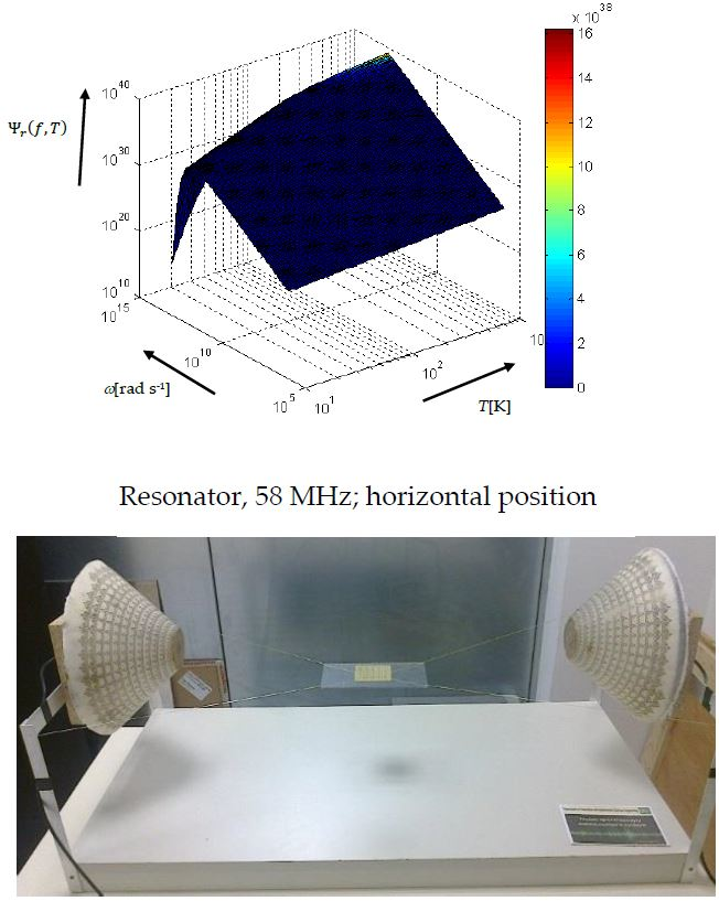
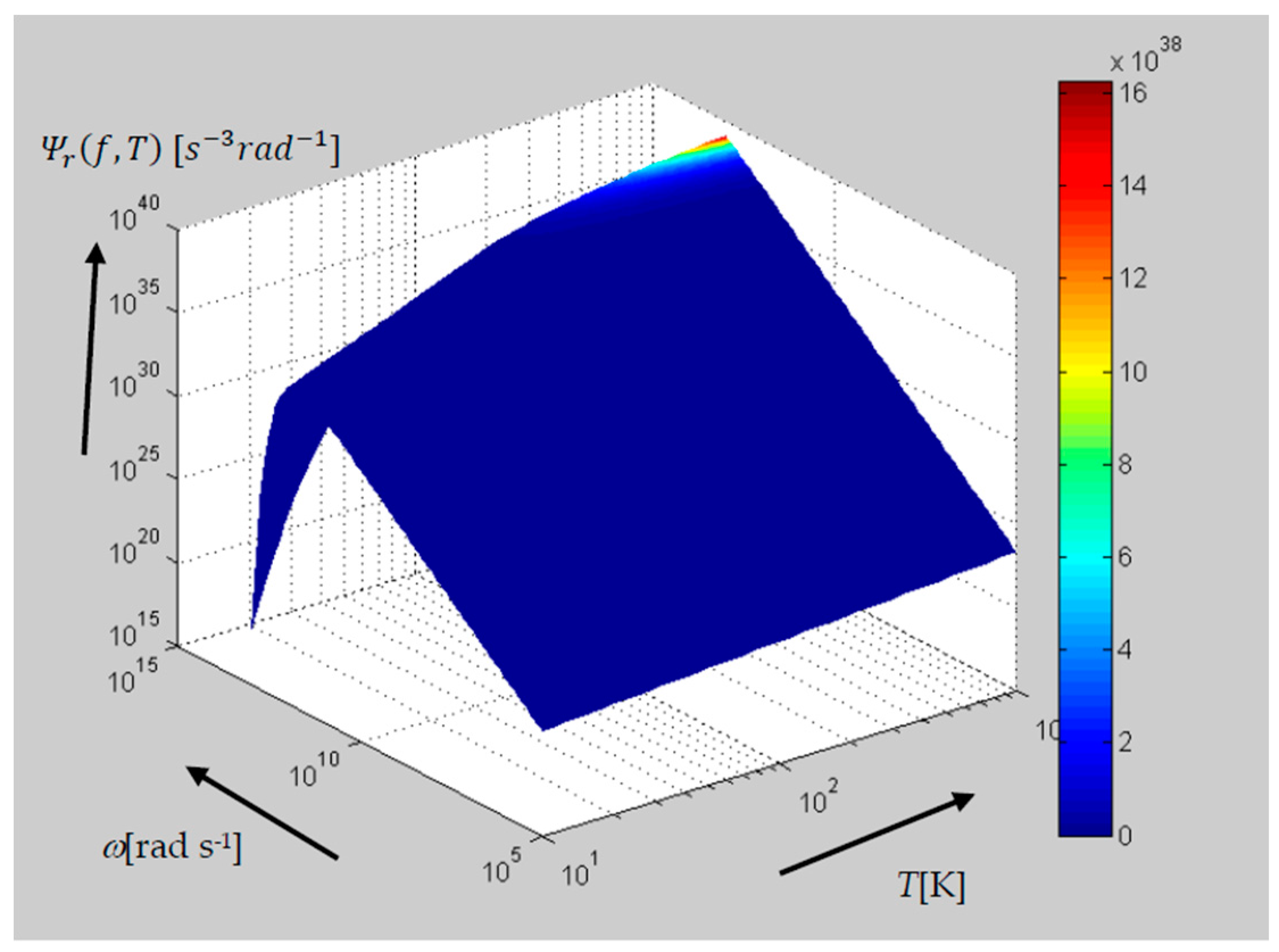
To evaluate the effect of the temperature T and the frequency 
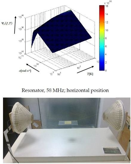
f on the radiated power, we have to consider the formula for expressing the distribution of the frequency spectrum from the above Equation (5); we then have
Ψ r ( f , T ) = ω 3 e ω h k T 1 .
This function assumes the form for Ψ r ( f , T ) shown in 
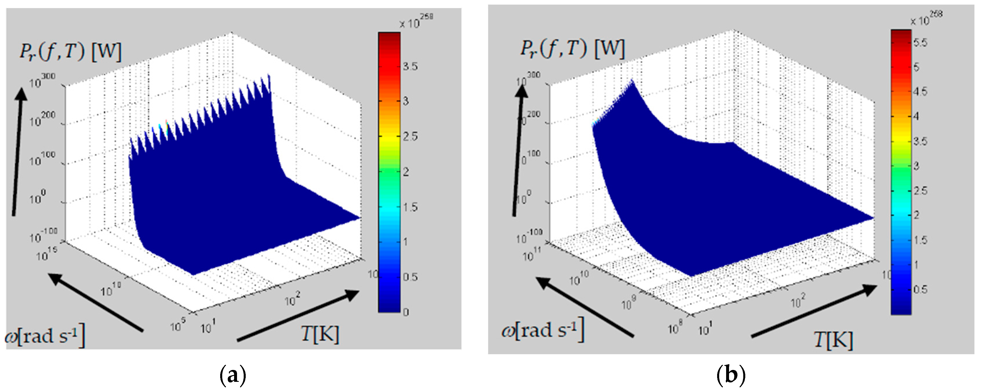
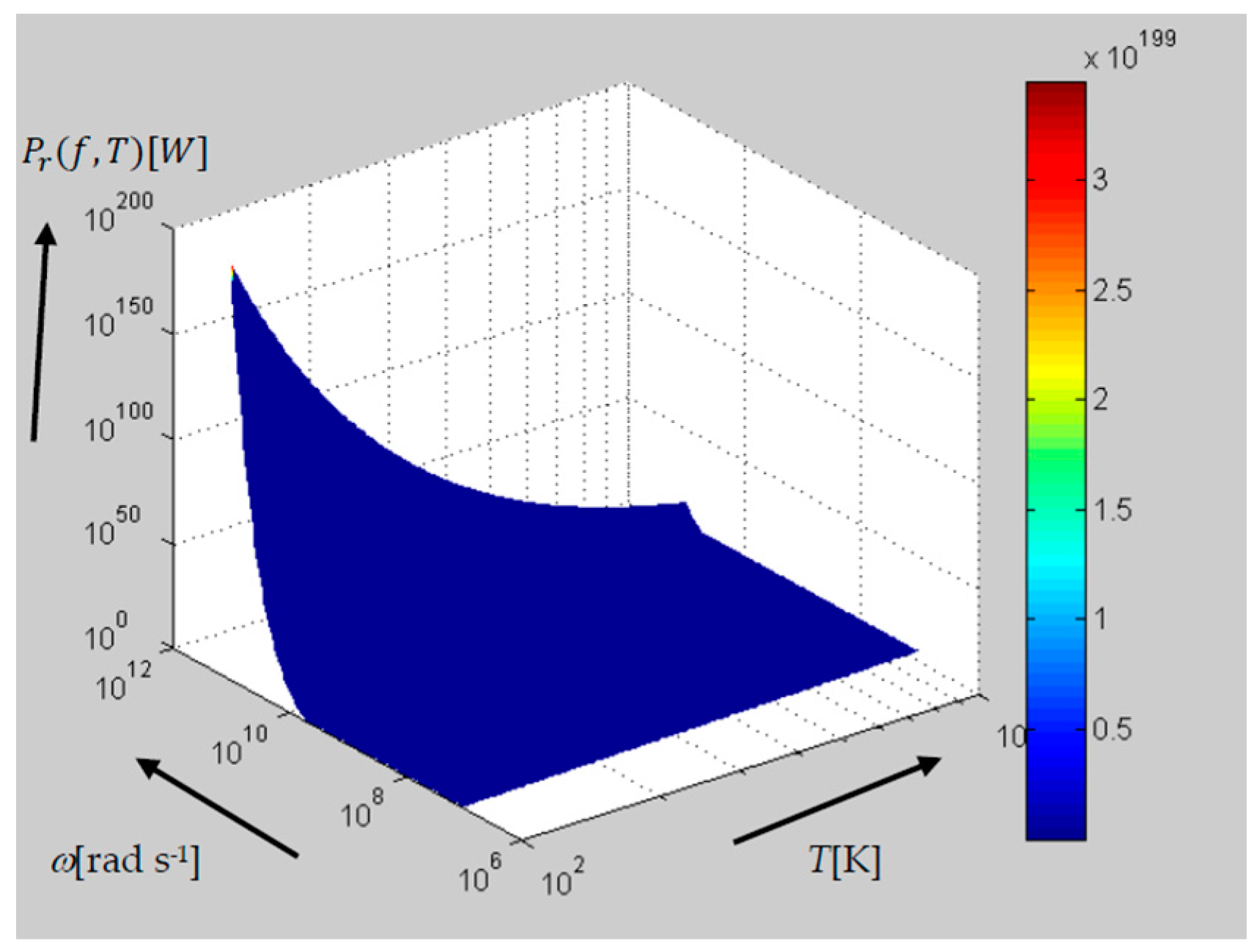
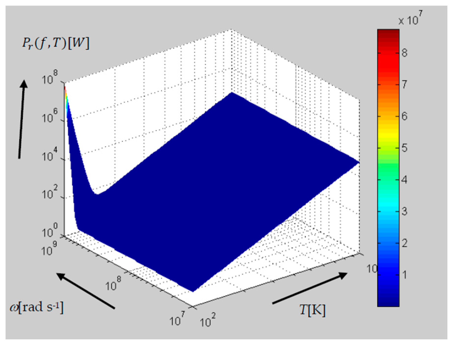
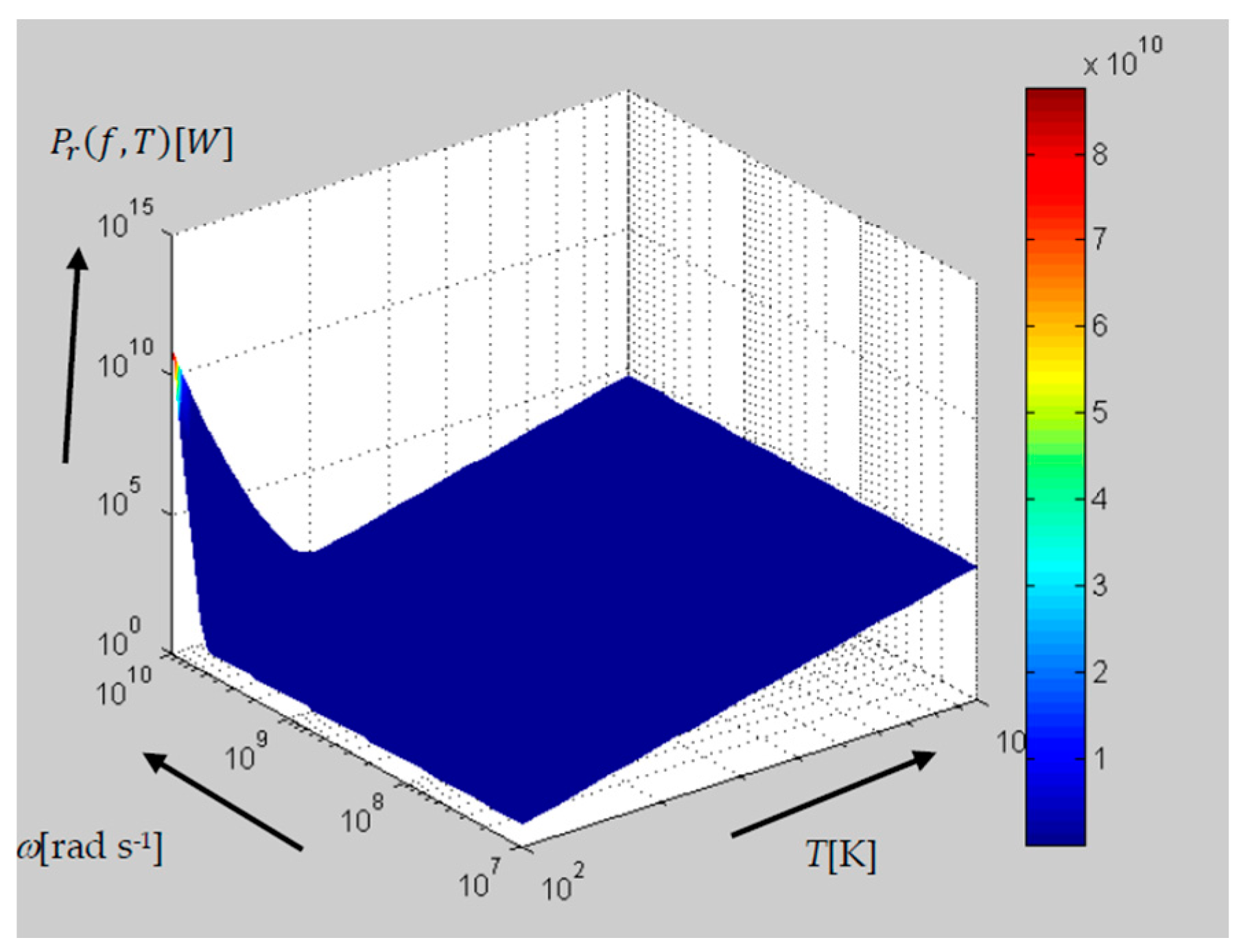
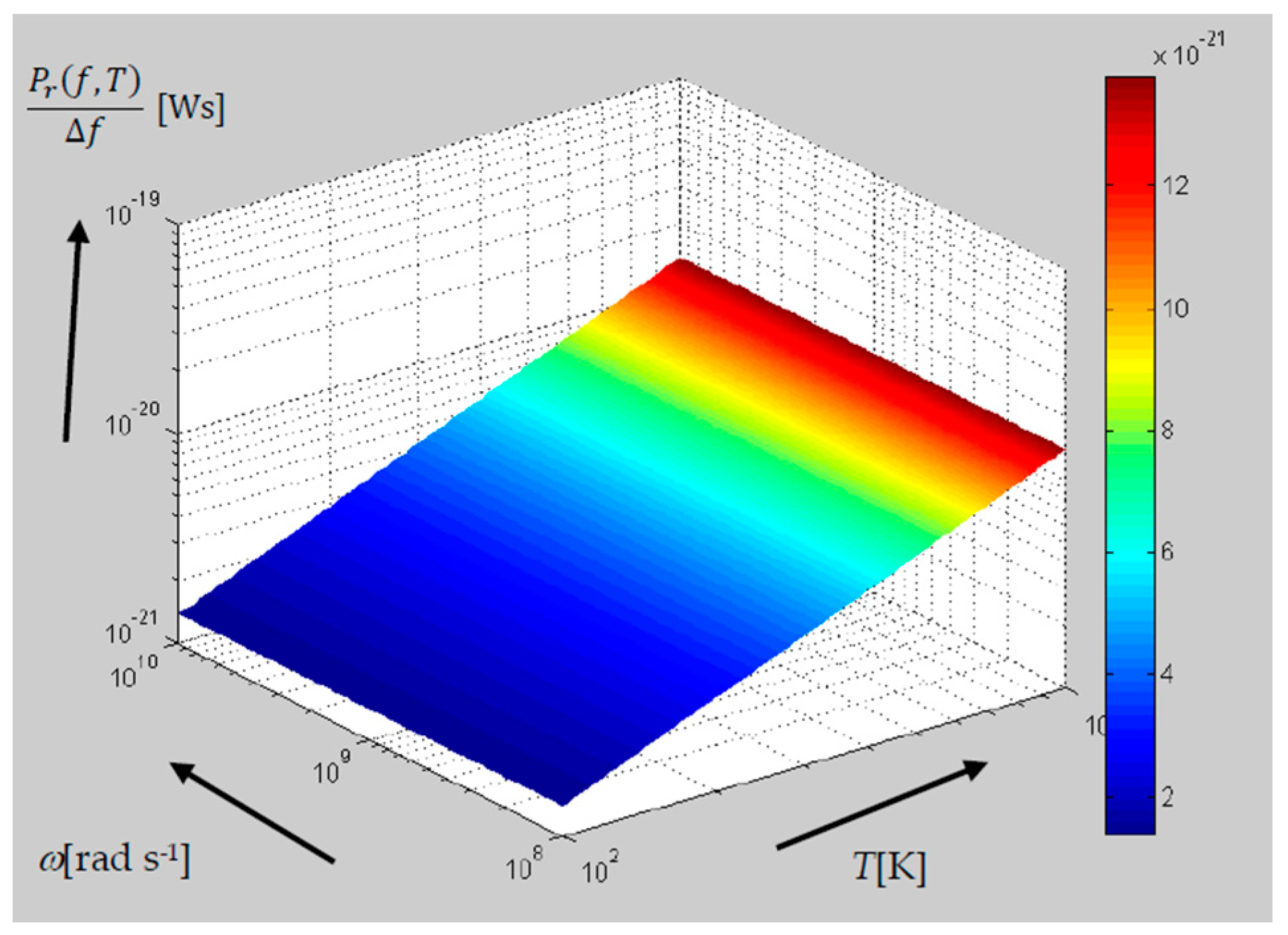
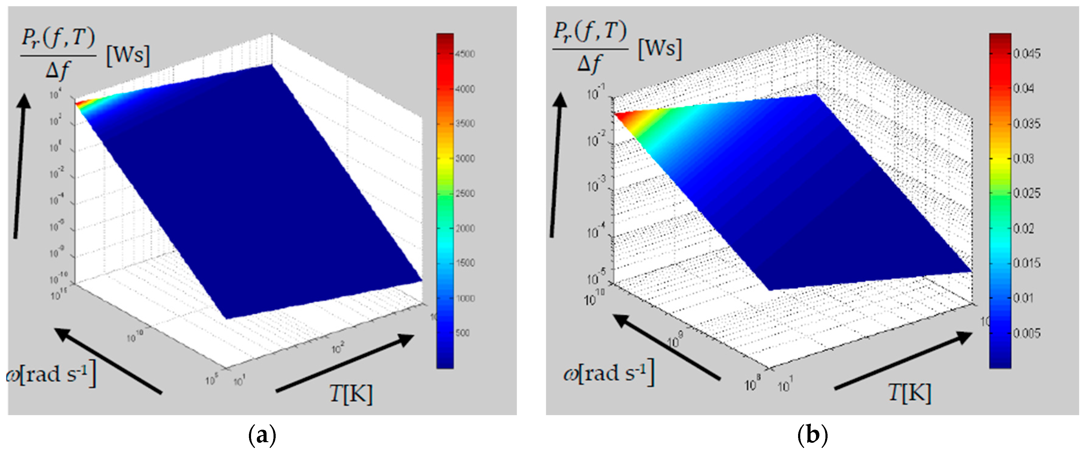
Figure 1. Specifying the formula for radiated power from Equation (8) will yield the expression
P r ( f , T ) = 2 π h c 2 S   ( 6 i = 1 e i ω h k T ( h k T ) 4 i 4 ω 4 4 + 3 ω 2 i = 1 e i ω h k T ( h k T ) 2 i 2 6 ω   i = 1 e i ω h k T ( h k T ) 3 i 3 + ω 3 ln ( 1 e ω h k T ) h k T ) .
Formula (11) for radiated power Pr can be graphically represented as the behavior for independent variables f and T, and this is shown in Figure 2, Figure 3, Figure 4 and Figure 5.
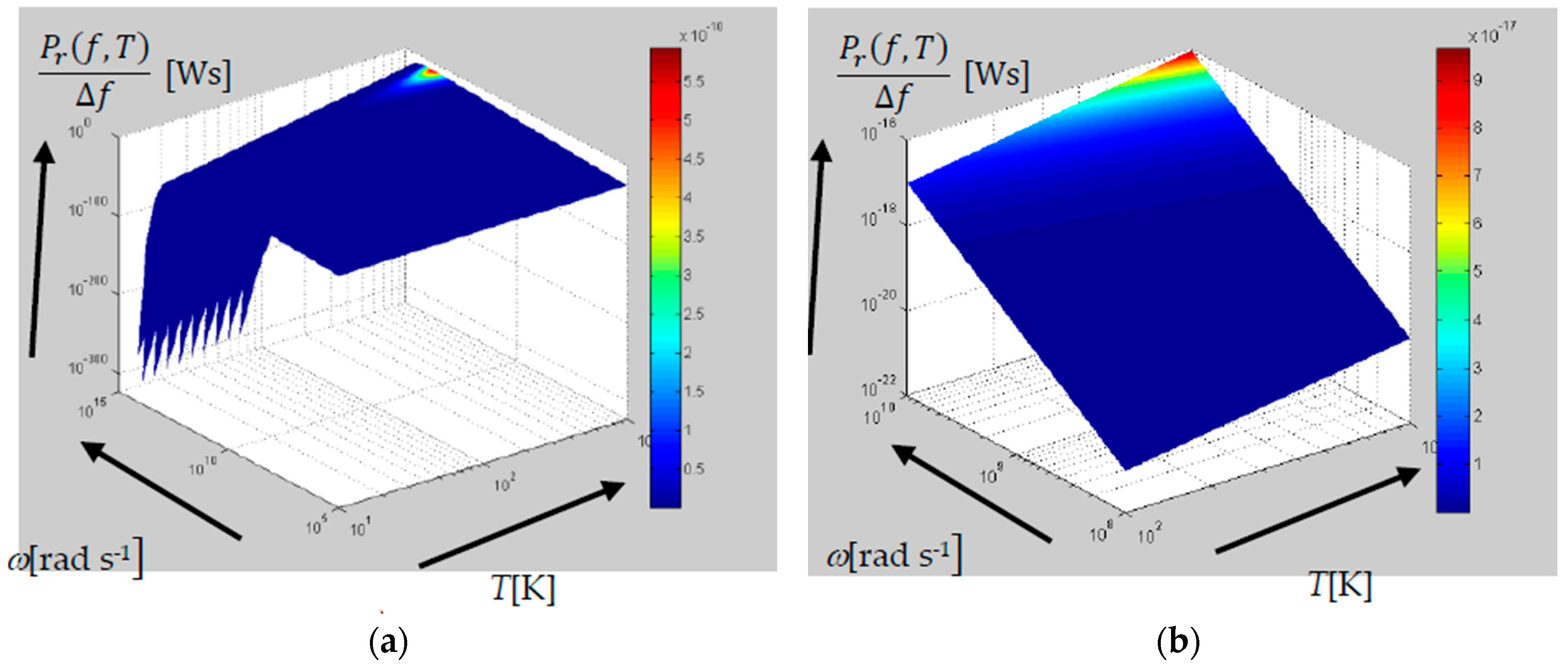
The power spectral density radiated by a half sphere (9) is presented in Figure 6. The power spectral density of noise generated by thermal, or Johnson–Nyquist, noise as a concept in communications technology [15] is formally written as
P r ( f , T ) f | f =   k T .
The relevant behavior is shown in Figure 7, exhibiting differences related to the frequency f. In analyses and evaluations with a limited frequency range, or one up to the order of GHz, the expression of the noise spectral density according to the Johnson–Nyquist formula constitutes, within the selected analyses, a tolerable deviation from the expression of an emitting black hemisphere. For higher frequencies, a more complex definition is used [14]:
P r ( f , T ) f | f ~   h ω k T e h ω k T 1 .
However, if the relationship between the power spectral density Pr/∆f and the frequency f has to be captured as either the broadband task or individual analyses, then, given that the frequency range f extends over several decades or reaches above 3 GHz, we can observe a difference between the simplified Expressions (12) and (13) and the one derived from the radiation of hemisphere (9). By extension, when comparing the spectral power densities represented in Figure 6, Figure 7 and Figure 8, we can also notice marked differences in the behavior of the functions. According to the relevant simplified criterion (12), power spectral density does not depend on the signal frequency f, but, as further outlined in Formula (9), the spectral density for half a sphere depends on the frequency (in a nonlinear manner). Interestingly, a comparison between the above Equation (9) for a hemisphere and the function derived by Nyquist will reveal a difference in the power of the frequency that determines the power spectral density of the signal, or noise; this finding subsequently enables us to explicate certain effects related to UWB and noise spectral tasks or, by extension, their analyses, estimates, predictions, real measurements, and experimental results.
From the perspective of the applied noise spectroscopy [5], it is then possible to conclude that the method is heavily nonlinear for higher frequency ranges (bandwidths) of noise, namely, those above 10 GHz. In the measuring method based on noise spectroscopy, the influence of the discussed dependence on the frequency f consists of the application of a noise spectrometer above tens of GHz up to units of THz, according to the evaluation of power spectral density outlined in (9), being nonlinear and thus highly frequency dependent. This precondition, therefore, has to be respected in any use of mathematical models consistent with the basic factors comprised in Table 1.
The above-presented views on the measurement accuracy may effectively explain certain deviations and error rates observed in the testing of metamaterials and periodic structures [5]; such deviations become evident through comparison with the results obtained from a swept spectrum analyzer for a spectral width larger than one decade.
Due to the error rate occurring at higher frequencies f within the region of tens of GHz if more than two decades are measured, it is not possible to evaluate the Johnson–Nyquist noise simply with the above Equation (12) or Equation (13); instead of these, we apply the above Formula (9) for a half sphere, derived from the Stefan–Boltzmann law, and observe the minimum radiated power above the limit of ambient noise. Where, however, the noise signal bandwidth remains less than a decade, the deviation between the two discussed approaches is not markedly conspicuous.

4. Experimental Comparison of Signal Properties for Noise Spectral Analyses

The theoretical conclusions following from the above-presented text may find various practical applications in, for example, noise spectroscopy laboratories [5]. The research into the usability of noise spectroscopy and methods for signal accumulation has pointed to certain properties of noise that can be analyzed quantitatively via the similarity of the white light of a broadband signal extending over at least several decades; such properties are describable according to the physical similarity from Table 1 and, in effect, reflect the differences within the relationship between the power spectral density of a hemisphere (9), spectral density of Johnson–Nyquist noise (12), and refined spectral density of Johnson–Nyquist noise (13).
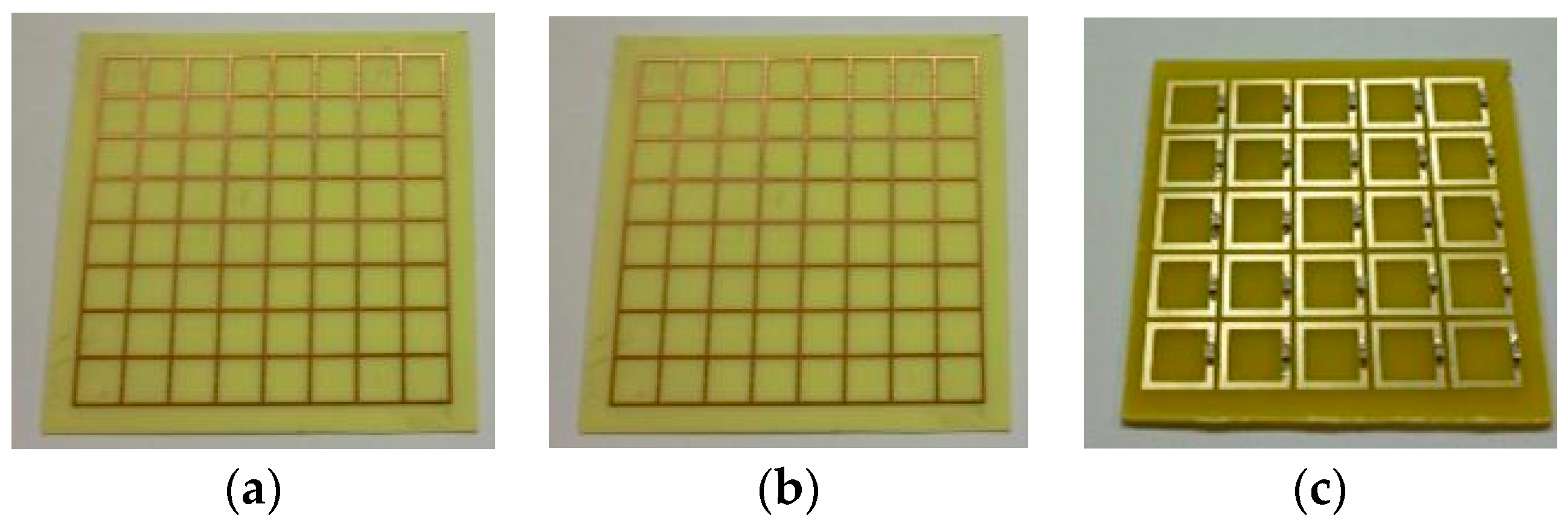
The research presented herein comprised the testing of material periodic structures exhibiting definable resonance characteristics; these structures were numerically analyzed [16,17] and their characteristics were experimentally measured with both a series (sequential) spectrum analyzer and noise spectroscopy. Such measurements then enabled us to compare not only the positive and negative features of the measuring methods but also the parameters required from the noise spectroscopy proper. In this context, we can then point to the samples from Figure 9 below.
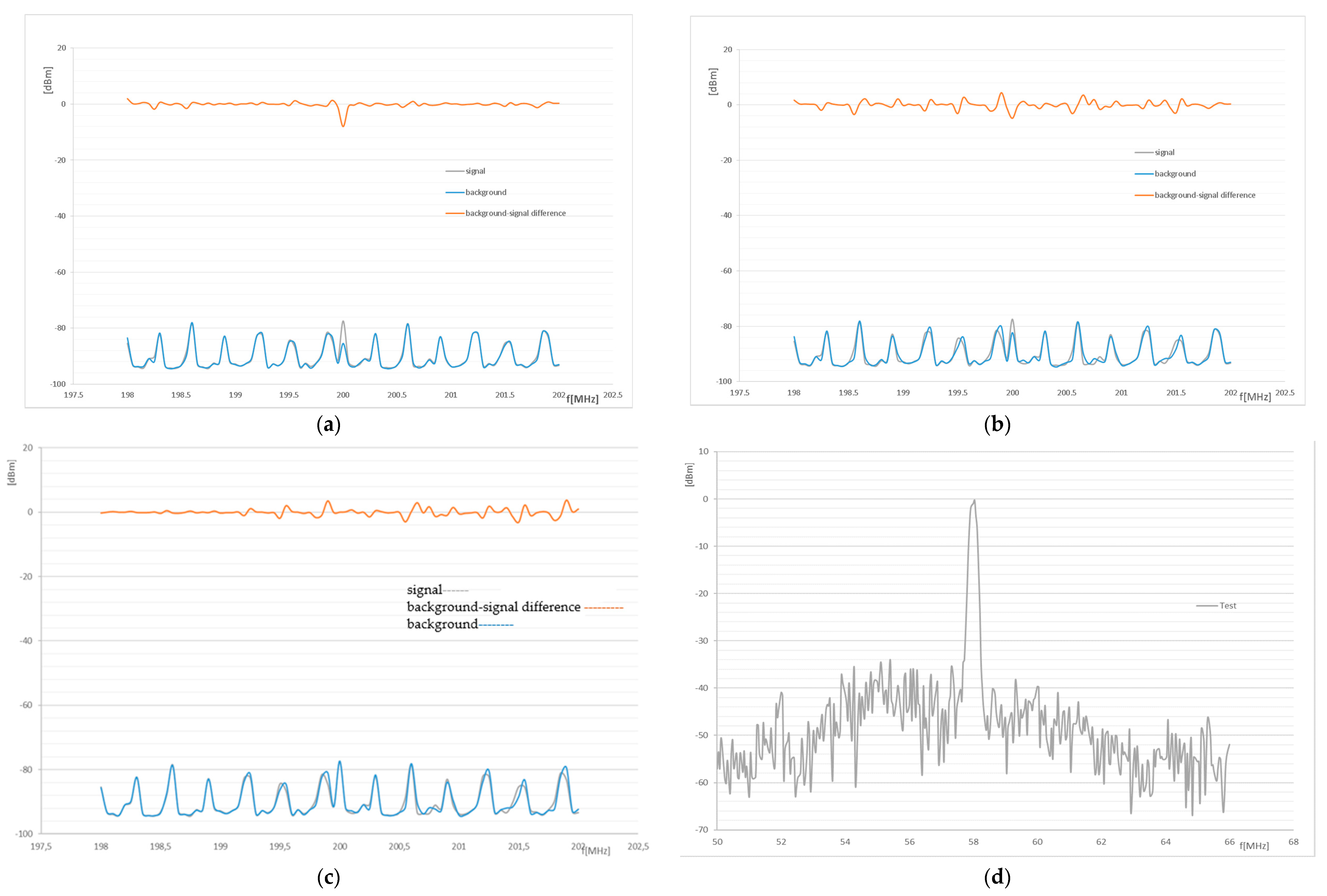
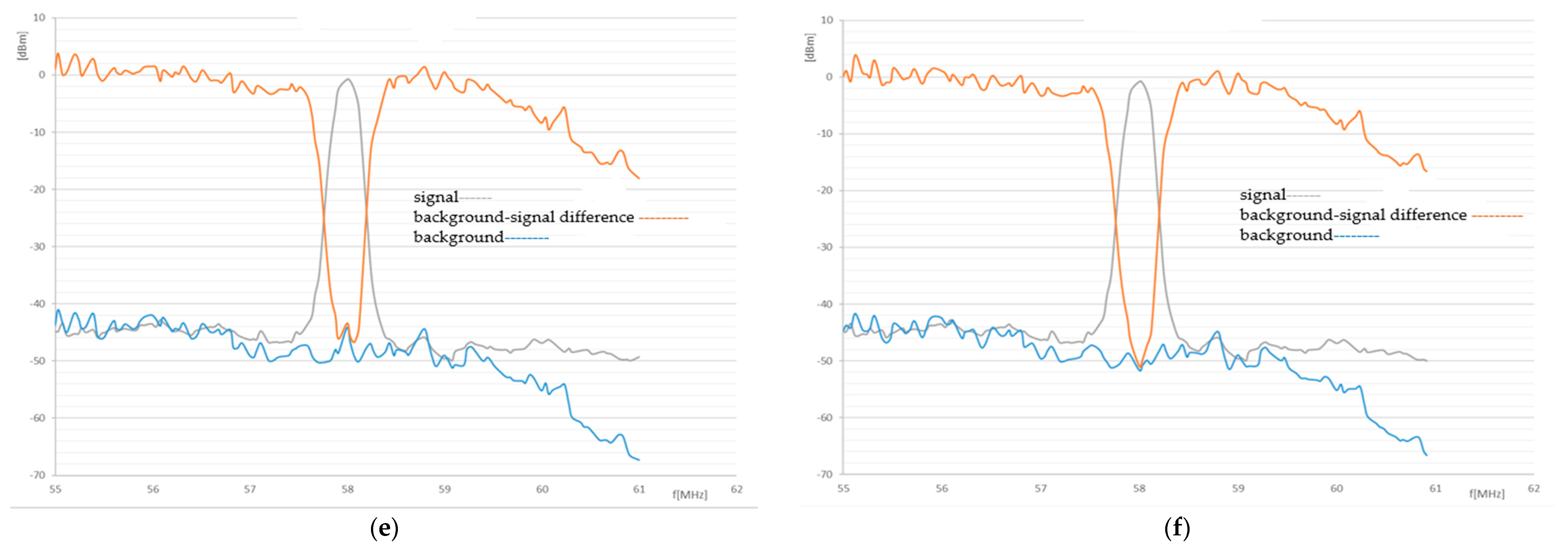
A major question relates to the noise signal strength that could facilitate effective evaluation and estimation of the properties of the examined sample. For this purpose, a simple test consisting of several steps can be performed. First of all, a signal having a known frequency ftest is conducted in the noise spectrometer area without the sample, and the spectrometer is employed to evaluate the variation of the signal with respect to the background. Thus, for example, the power of the noise signal was changed from 22 dBm (Figure 10a) through 30 dBm (Figure 10b), 70 dBm (Figure 10c), 70 dBm (Figure 10d), and 105 dBm (Figure 10e) to 127 dBm (Figure 10f). The results of the given test are indicated in Figure 10. The relevant experimental measurements make it possible to estimate the power rates to be achieved in a chain comprising a noise generator, an amplifier, and an antenna in order to secure such conditions for the given noise spectral analysis that will facilitate the cumulation of the required frequency characteristics of the tested samples.
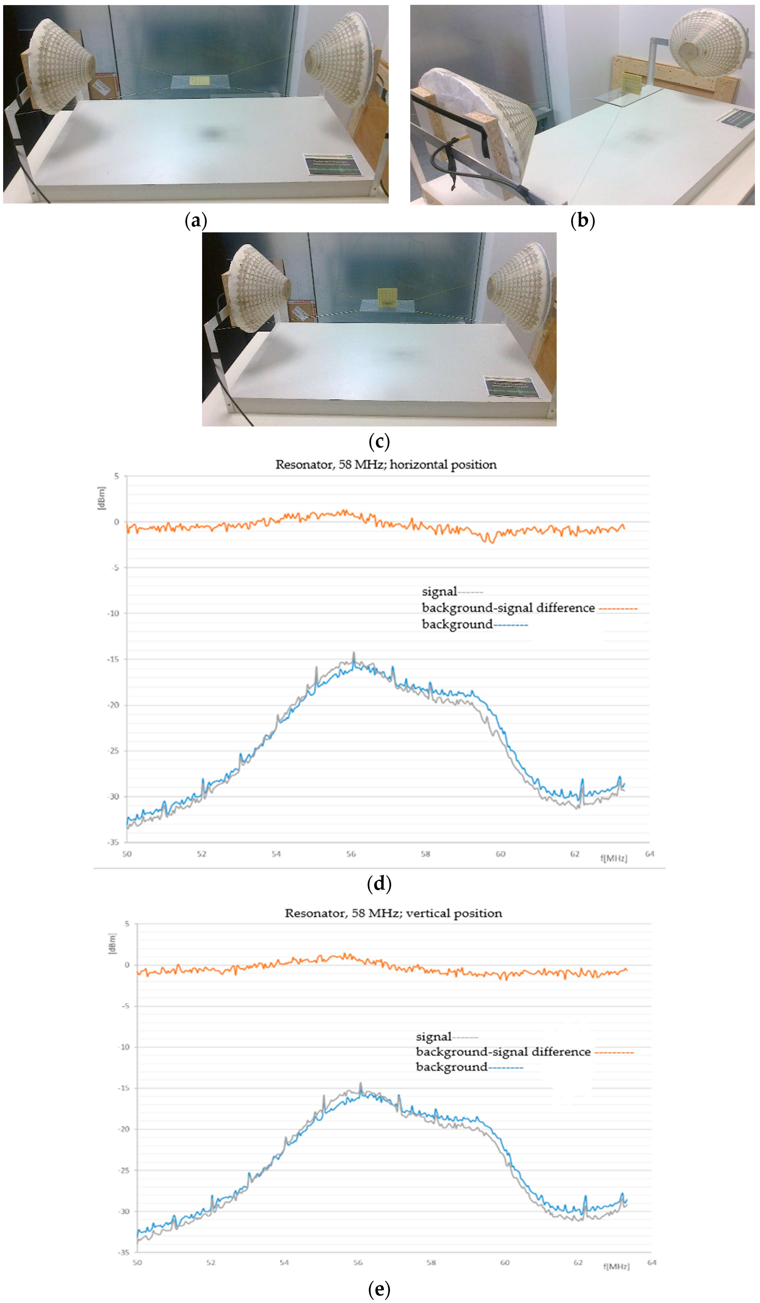
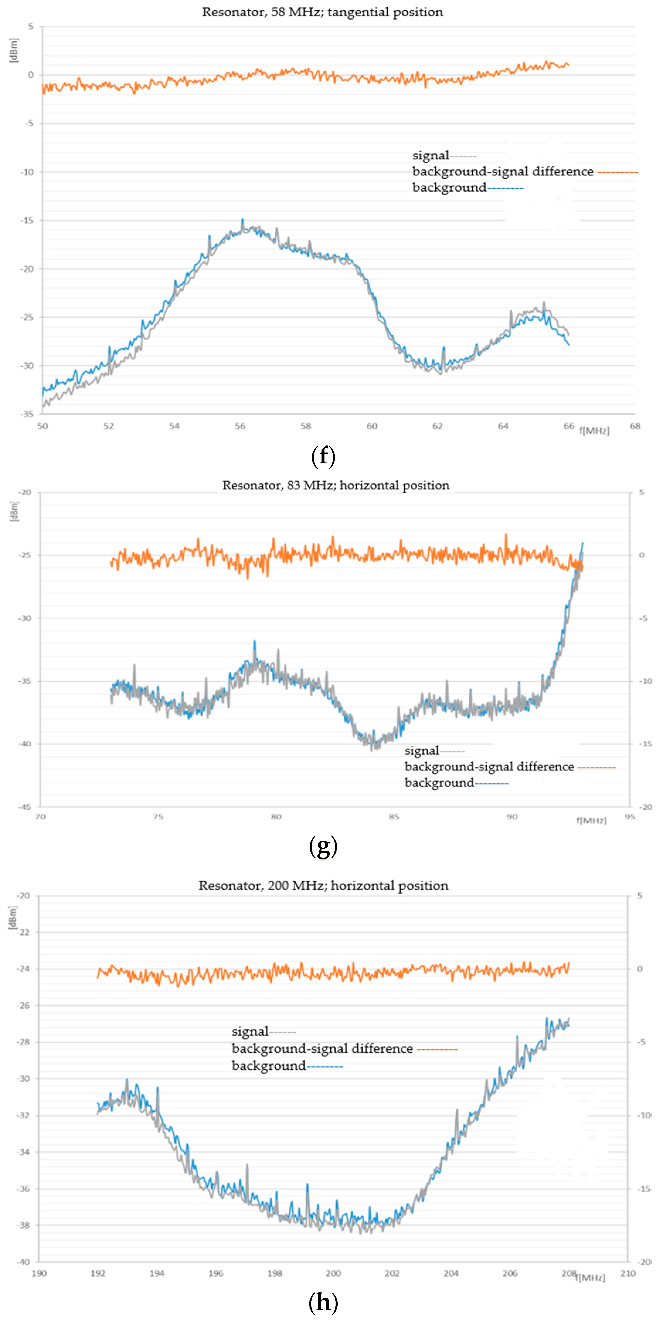
In the testing of the samples from Figure 9, with setting for the states indicated in Figure 10, the results of the noise analysis of the periodic structures can be interpreted within Figure 11.
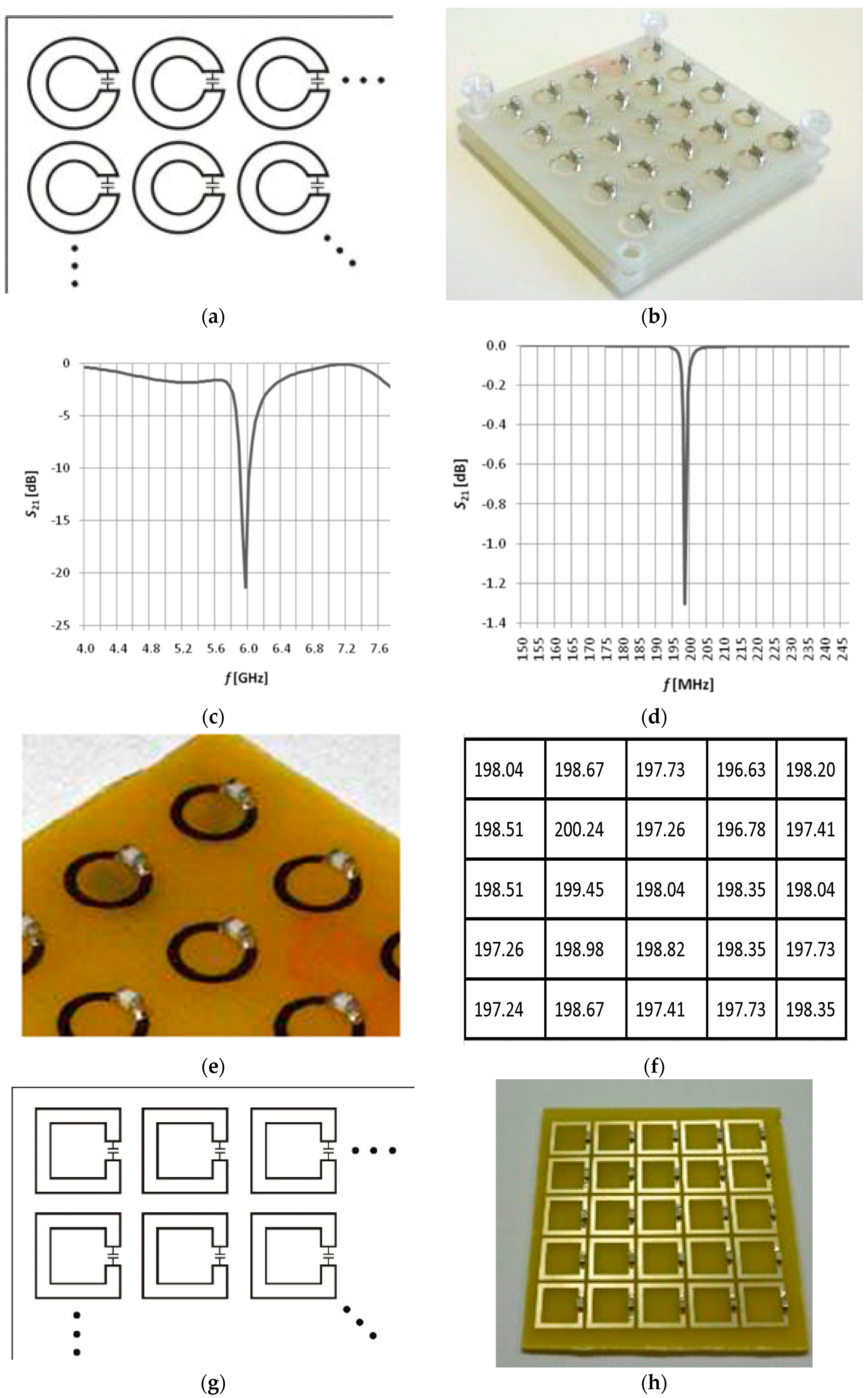
The tests and partial experiments indicated the necessity to use a generator–amplifier–antenna chain exhibiting a gain higher than 10 dBm; such a value embodies the precondition for the method to yield processable results markedly overriding the background noise. Within the research, we tested various types of resonant structures and their properties in diverse frequency bands. Selected resonant structures are presented in Figure 12, together with the relevant numerical characteristics (verified via spectrum analyzers).

5. Conclusions

The paper proposes a novel approach to noise as a tool of spectroscopy, comprising a unique, compact set of theoretical and experimental results obtained from research into the noise field. In this context, the article presents an overview of the laboratory equipment for noise spectroscopy measurement and the related experiments. The authors discuss various approaches to models for evaluating the parameters related to the quantification character of the application of noise in noise spectroscopy. With respect to the experiments and laboratory-based testing, the present report notices relevant limiting aspects, including the radiated power of a broadband transmission system to ensure the minimal gain of signals in the monitored spectrum; the purpose of this process then consists of securing the evaluation of major information and the parameters of the tested periodic structure.
The research performed by the authors within UWB signals is oriented towards subregions such as non-destructive diagnostics of classic materials or structures; its practical applicability lies in the evaluation of materials as periodic systems (currently represented by benzene core-based nanomaterials, amorphous magnetic materials, and similar substances) and within security systems or concepts. The set of aspects evaluable via the proposed technique also includes the quality of products manufactured from complex polymeric organic materials. The investigation procedures exploit known properties of several effects, including noise as a UWB signal, the response of identical structures, and changes in the spectra of signals; a relevant advantage is embodied in the possibility of conducting the research without the necessity to use an anechoic chamber and other highly specialized laboratories.

Acknowledgments

The research described in this paper was financed by the Czech Science Foundation under Grant No. 13-09086S and National Sustainability Program under grant No. LO1401. For the actual analyses and experiments, the infrastructure of the SIX Center was used.

Author Contributions

Pavel Fiala contributed to the analyzed theoretical problem and wrote the paper; Petr Drexler, Dusan Nespor, and Zoltan Szabo conceived and designed the experiments; Jan Mikulka prepared the signal analyses and evaluation; and Jiri Polivka provided his opinions on the radioelectronics related to noise and noise technologies.

Conflicts of Interest

The authors declare no conflict of interest. The sponsors had no role in the design of the study; in the collection, analyses, or interpretation of the data; in the writing of the manuscript; or in the decision to publish the results.

References

  1. Hollas, J.M. Modern Spectroscopy; Wiley: New York, NY, USA, 2004. [Google Scholar]
  2. Regadio, A.; Tabero, J.; Sanchez-Prieto, S. Impact of colored noise in pulse amplitude measurements: A time-domain approach using differintegrals. Nuceal Instrum. Methods Phys. Res. Sect. A 2016, 811, 25–29. [Google Scholar] [CrossRef]
  3. Nasswettrova, A.; Drexler, P.; Seginak, J.; Nešpor, D.; Friedl, M.; Marcoň, P.; Fiala, P. Noise Spectroscopy of Nano- and Microscopic Periodic Material Structures. In Proceedings of the SPIE—Smart Sensors, Actuators, and MEMS VII, Barcelona, Spain, 4–6 May 2016.
  4. Fiala, P.; Machac, J.; Polivka, J. Microwave noise field behaves like white light. Prog. Electromagn. 2011, 111, 311–330. [Google Scholar]
  5. Drexler, P.; Seginak, J.; Mikulka, J.; Nespor, D.; Szabo, Z.; Marcon, P.; Fiala, P. Periodic material structures tested by the noise spectroscopy method. Microsyst. Technol. 2016, 22, 2783–2799. [Google Scholar] [CrossRef]
  6. Figlus, T.; Gnap, J.; Skrucany, T.; Sarkan, B.; Stoklosa, J. The use of denoising and analysis of the acoustic signal entropy in diagnosing engine valve clearance. Entropy 2016, 18, 253. [Google Scholar] [CrossRef]
  7. Yang, T.; Liu, S.; Tang, M.; Zhang, K.; Zhang, X. Optimal noise enhanced signal detection in a unified framework. Entropy 2016, 18, 213. [Google Scholar] [CrossRef]
  8. Siddagangaiah, S.; Li, Y.; Guo, X.; Chen, X.; Zhang, Q.; Yang, K.; Yang, Y. A complexity-based approach for the detection of weak signals in ocean ambient noise. Entropy 2016, 18, 101. [Google Scholar] [CrossRef]
  9. Li, C.; Zhan, L.; Shen, L. Friction signal denoising using complete ensemble EMD with adaptive noise and mutual information. Entropy 2015, 17, 5965–5979. [Google Scholar] [CrossRef]
  10. Kadlecova, E. Automated System of Calculation of Reflecting Surface of Light Sources. Ph.D. Thesis, Brno University of Technology, Brno, Czech Republic, 2005. [Google Scholar]
  11. Kadlec, R.; Fiala, P.; Behunek, I. Response of a Layered Medium to an Obliquely Incident Wave. In Proceedings of the Progress in Electromagnetics Research Symposium, Stockholm, Sweden, 12–15 August 2013.
  12. Kadlec, R.; Fiala, P. The response of layered materials to EMG waves from a pulse source. Prog. Electromagn. Res. M 2015, 42, 179–187. [Google Scholar] [CrossRef]
  13. Husain, V.; Seahra, S.S.; Webster, E.J. High energy modifications of blackbody radiation and dimensional reduction. Phys. Rev. D 2013, 88, 024014. [Google Scholar] [CrossRef]
  14. Nyquist, H. Thermal agitation of electric charge in conductors. Phys. Rev. 1928, 32, 110. [Google Scholar] [CrossRef]
  15. Risken, H. The Fokker–Planck Equation: Methods of Solution and Applications; Springer: Berlin, Germany, 1996. [Google Scholar]
  16. Nespor, D.; Drexler, P. Magnetic Field Shaping with Quasi-Periodic Resonators. In Proceedings of the Progress in Electromagnetics Research Symposium, Prague, Czech Republic, 6–9 July 2015.
  17. Nespor, D.; Drexler, P.; Fiala, P.; Marcon, P. RF Resonator Array for MR measurement system. In Proceedings of the 10th International Conference on Measurement, Bratislava, Slovakia, 25–28 May 2015.
Figure 1. The behavior of function Ψ r ( f , T ) , with the frequency range of f ~0.1 MHz–1000 THz and temperature of T = 10–1000 K.
Entropy 18 00443 g001
Figure 2. The behavior of radiated power Pr [W]: (a) the frequency range of f ~0.1 MHz–1000 THz and temperatures T between 10 and 1000 K; (b) the behavior of radiated power Pr [W] in the frequency range of f ~100 MHz–100 GHz and at temperatures of T = 10–1000 K.
Entropy 18 00443 g002
Figure 3. The behavior of radiated power Pr [W] in the frequency range of f ~10 MHz–10 GHz and at temperatures of T = 100–1000 K.
Entropy 18 00443 g003
Figure 4. The behavior of radiated power Pr [W] in the frequency range of f ~10 MHz–1 GHz and at temperatures of T = 100–1000 K.
Entropy 18 00443 g004
Figure 5. The behavior of radiated power Pr [W] in the frequency range of f ~10 MHz–1 GHz and at temperatures of T = 100–10,000 K (relation (11)).
Entropy 18 00443 g005
Figure 6. The behavior of power spectral density Pr/∆f [Ws]: (a) the frequency range of f ~0.1 MHz–1000 THz and temperatures between 10 and 1000 K, according to relation (9); (b) in the frequency range of f ~100 MHz–10 GHz and at temperatures of T = 100–1000 K, from Planck’s law of a black body, relation (9).
Entropy 18 00443 g006
Figure 7. The behavior of power spectral density Pr/∆f [Ws] in the frequency range of f ~100 MHz–10 GHz and at temperatures of T = 10–100 K, related to Johnson–Nyquist noise, relation (12).
Entropy 18 00443 g007
Figure 8. The behavior of power spectral density Pr/∆f [Ws]: (a) the frequency range of f ~0.1 MHz–1000 THz and temperatures between 10 and 1000 K, according to the Nyquist–Planck Formula (13); (b) related to the Nyquist–Planck Formula (13); the frequency range of f ~100 MHz–10 GHz and temperatures of T = 10–100 K.
Entropy 18 00443 g008
Figure 9. The tested samples of periodic structures: the expected resonant frequencies of the first mode: (a) resonator f11 = 58 MHz; (b) resonator f12 = 83 MHz; (c) resonator f13 = 200 MHz.
Entropy 18 00443 g009
Figure 10. The test of the noise spectroscopy setup with respect to the power of the excitation signal at one frequency: (a) the background checking, 198–202 MHz; the generator signal of 200 MHz–22 dBm, without an amplifier—number of samples: 2000; (b) the background checking, 198–202 MHz; the generator signal of 200 MHz–30 dBm, without an amplifier—number of samples: 2000; (c) the background checking, 198–202 MHz; the generator signal of 200 MHz–70 dBm, without an amplifier—number of samples: 10,000; (d) the test generator: signal of 58 MHz–70 dBm (noise level signal); input: a +27 dBm amplifier; output: a two-stage electronic radio-frequency amplifier (ERA) ; (e) the test generator: signal of 58 MHz–105 dBm (signal immersed in noise); input: a +27 dBm amplifier; output: a two-stage ERA—number of samples: 5000; (f) the test generator: signal of 58 MHz–127 dBm (signal immersed in noise); input: a +27 dBm amplifier; output: a two-stage ERA—number of samples: 5000.
Entropy 18 00443 g010aEntropy 18 00443 g010b
Figure 11. The testing of the samples from Figure 9 with noise spectroscopy: (a) the noise generator: horizontal configuration; (b) the noise generator: vertical configuration; (c) the noise generator: tangential configuration; (d) the noise generator: a TVA amplifier +27 dBm; an antenna–an antenna –a two-stage ERA amplifier–an Agilent spectrometer (Keysight Technologies, Inc., Westlake Village, CA, USA); a sample from Figure 9. f11, horizontal position, 58 MHz; (e) the noise generator: a TVA amplifier +27 dBm; an antenna–an antenna–a two-stage ERA amplifier–an Agilent spectrometer; a sample from Figure 9. f11, vertical position; (f) the noise generator: a time variant amplifier (TVA) + 27 dBm; an antenna–an antenna–a two-stage ERA amplifier–an Agilent spectrometer; a sample from Figure 9. f11, tangential position; (g) the noise generator: a TVA amplifier + 27 dBm; an antenna–an antenna–a two-stage ERA amplifier–an Agilent spectrometer; a sample from Figure 9. f12, horizontal position; (h) the noise generator: a TVA amplifier + 27 dBm; an antenna–an antenna–a two-stage ERA amplifier–an Agilent spectrometer; a sample from Figure 9. f13, horizontal position.
Entropy 18 00443 g011aEntropy 18 00443 g011b
Figure 12. The design and types of the samples tested for noise spectroscopy: (a) the design; (b) the fabricated unit; (c) the frequency dependence without a capacitor; (d) the frequency dependence with capacitors; (e) a detailed view of the tuned structure; (f) the resonance values measured over elementary resonators; (g) the magnetic imaging (MI) lens designed with square resonators [16,17]; (h) the fabricated MI-based unit; (i) the resonant structure consisting of two plates with quasi-periodic resonators: fr = 58 MHz; (j) and fr = 83 MHz.
Entropy 18 00443 g012aEntropy 18 00443 g012b
Table 1. The mutual relationship between thermal and light quantities.
Heat (λ ∈ <780;10,000> nm)White Light (λ ∈ <440;780> nm)
Monochromatic (spectral) radiation [W·m−1]
H λ = d W λ d λ
Monochromatic (spectral) luminous flux [W·m−1]
Φ λ = d Φ e d λ
Radiant flux [W]
Φ e = S   H e d S , H e = 0 H λ d λ
Radiant flux [W]
Φ e = 0 Φ λ d λ
Radiant intensity [W·sr−1]
I = d Φ e d ω
Luminous intensity [W·sr−1]
I e = d Φ e d ω
Radiance [W·m−2·sr−1]
L e = d I e d S   c o s ϑ
Luminance [W·m−2·sr−1]
L e = d I ϑ d S   c o s ϑ
Radiant exposure [W·m−2]
H e = d Φ e d S
Luminous exitance [W·m−2]
H = d Φ e d S
Irradiance [K·s·m−1]
E e = d Φ e d A
Illuminance [K·s·m−1]
E s = d Φ e d A
Thermal flux [W·s·m−2]
ϕ T = k T   grad   T
Luminous flux [W·s·m−2]
ϕ = K m 0 V λ ϕ λ d λ

