Nonparametric Problem-Space Clustering: Learning Efficient Codes for Cognitive Control Tasks

Abstract

We present an information-theoretic method permitting one to find structure in a problem space (here, in a spatial navigation domain) and cluster it in ways that are convenient to solve different classes of control problems, which include planning a path to a goal from a known or an unknown location, achieving multiple goals and exploring a novel environment. Our generative nonparametric approach, called the generative embedded Chinese restaurant process (geCRP), extends the family of Chinese restaurant process (CRP) models by introducing a parameterizable notion of distance (or kernel) between the states to be clustered together. By using different kernels, such as the the conditional probability or joint probability of two states, the same geCRP method clusters the environment in ways that are more sensitive to different control-related information, such as goal, sub-goal and path information. We perform a series of simulations in three scenarios—an open space, a grid world with four rooms and a maze having the same structure as the Hanoi Tower—in order to illustrate the characteristics of the different clusters (obtained using different kernels) and their relative benefits for solving planning and control problems.

1. Introduction

Learning efficient codes or representations of the environment is a key prerequisite for several cognitive tasks. In vision research, information-theoretic and statistical methods have been successfully used to study the coding properties of visual cortex neurons [1]. Here, a key assumption is that these neurons are sensitive to the natural statistics and information content of visual scenes and encode them efficiently in an information-theoretic sense [2]. If we apply the same logic to neural coding besides vision, it is plausible that brain areas that have different inputs/outputs (and computational demands) are sensitive to the different kinds of statistical regularities to which they are exposed, especially if one conceives of the brain as a statistical machine [3].

In artificial intelligence (AI), reinforcement learning (RL) and related areas, it has been long known that learning to code the problem space efficiently is paramount to finding efficient solutions [4,5,6]. While in several practical AI and RL applications, the so-called state-space is provided by programmers by hand, for example in the form of a grid of discrete cells that cover the whole space, it is not guaranteed that this is the most efficient representation to solve the problem at hand. Indeed, a recent approach consists of learning these representations using unsupervised methods, such as deep learning, a method that has been successful in improving the performance of RL agents [7].

Furthermore, recent computational studies have shown that using information measures to find structure in the environment, for example in the form of bottlenecks of sub-goals that permit splitting navigation problems into subproblems, improves planning efficiency and lowers the demands (e.g., memory and cognitive load) of artificial agents [8,9,10,11]. These and other studies link well with empirical studies showing that humans are indeed sensitive to the structure of their environment [12].

Therefore, from both a cognitive (neuro)science and a computational modeling perspective, a key problem is how to find structure in the problem space. For most artificial agents, which solve multiple problems simultaneously, this problem holds at various levels of complexity, from the problem of visually recognizing and categorizing objects (analogous to the vision studies reviewed earlier), to the problem of navigating, exerting efficient cognitive control, etc.

In analogy with the case of information approaches to vision discussed above, one might ask which are the most important regularities, or in other words, what the natural statistics of control tasks are. We hypothesize that control tasks are multifarious and might pose different demands, from the identification of a path to a known goal, to the recognition of possible sub-goals, and that each problem can benefit from a different task coding or decomposition. Therefore, one might need a flexible system that selects the most appropriate representation depending on the task at hand. Along these lines, recent neuroscientific evidence suggests that prefrontal codes are indeed sensitive to multiple dimensions of the stimuli [13] and might quickly adapt to novel task demands, such as the identification of specific goals [14,15,16,17,18].

In this article, we address the problem of finding efficient codes for various cognitive control tasks from a computational perspective. We present a general information-based method to cluster and split the problem space into ways that make control problems more efficient. To this aim, we introduce a novel nonparametric approach: the generative embedded Chinese restaurant process (geCRP). This approach builds on a variant of the Chinese restaurant process (CRP) [19], the distance-dependent CRP [20], in which the notion of distance is added to the CRP to cope with situations in which several observations mutually influence each other. We further generalize the distance-dependent CRP by using model-based discriminant functions (generative kernels) instead of the notion of distance, in such a way as to embed prior information on observations about how the data were generated.

Here, we show that different parametrizations of the geCRP method permit one to derive task clusterings that are more sensitive to different control-related information, such as goal, sub-goal and path information. To support our analysis, we show that each of the resulting task clusterings has specific benefits for a class of control problems, including planning a path to a goal from a known location, from an unknown location, the achievement of multiple goals and the exploration of a novel environment.

2. Methods

Traditionally, clustering techniques can be grouped into parametric and nonparametric [21]. In the first ones, the clustering process is viewed as a density estimation of a mixture distribution for whose components (the clusters) a specific parametric form has to be assumed (a Gaussian one, quite commonly). This means restricting the clusters’ shapes to a precise statistical distribution family, and this can compromise the result. In particular, the standard K-means approach and its popular derivations crucially require the number of clusters to be fixed in advance [22]. Nonparametric approaches do not have such strong constraints. Unlike parametric ones, nonparametric approaches make no assumptions about the probability distributions of the variables being assessed. The difference between parametric methods and nonparametric methods is that in the latter, the number of parameters is potentially infinite and is determined by data, not by the model. Despite this, nonparametric approaches use some meta-parameters governing the inference of the correct form and size of the model.

Our starting point is a recently introduced generative nonparametric mixture: the Chinese restaurant process (CRP) [19]. CRP has proven to be able to infer the number of clusters from the data and to be an effective tool for mining information from high dimensional data. Specifically, we leverage a variant of CRP and extend it, using a framework that permits one to define algorithmic probability distributions on discrete states. Below, we introduce the original CRP methods and the ways we extended them.

2.1. Distance-Dependent Chinese Restaurant Process

The CRP [19] is a generative process determining prior distributions over infinite partitions of combinatorial structures. The name “CRP” derives from the metaphor commonly used to describe this stochastic process: a sequence of N customers enters a Chinese restaurant with an infinite number of tables; they sit down randomly at a table with a probability depending on the number of the customers already occupying it. The assignment of customers to tables represents a random partition where tables are blocks and customers are elements of the set $\{1,\cdots ,N\}$ partitioned.

More formally, we can denote as $z_i$ the table assignment of the i-th customer; i occupies the table k with $n_k$ customers already sitting according to the distribution:

$$p(z_i=k|z_{1:(i-1)},\alpha )\propto \left\{\begin{array}{ccc}\alpha \hfill & \mathrm{if}\hfill & k=T+1\hfill \\ n_k\hfill & \mathrm{if}\hfill & k\le T\hfill \end{array}\right.$$

(1)

where $z_{1:(i-1)}$ is the assignment of the previously entered customers occupying T tables and α is a concentration parameter controlling the probability of the i-th customer to choose an unoccupied table. In practice, a larger α favors partitions with more tables.

An important feature of CRP is the marginal invariance: the probability distribution over partitions does not depend on the ordering of the customers entering in the restaurant. This property theoretically links CRP to the Dirichlet process (DP) mixture model [23], a Bayesian nonparametric mixture model that is widely used to design flexible clustering algorithms for high-dimensional data analysis.

However, in problems (like the ones we face here) where observations mutually influence each other, marginal invariance needs to be relaxed. Several generalizations of CRP allow for non-exchangeable distributions on partitions [24,25,26,27]. Among these methods, the distance-dependent CRP (ddCRP) [20] is one of the most widely used. Different from the CRP, in which the table assignment $z_i$ is directly modeled, ddCRP recreates table assignments based on the linkage between customers.

Using a “culinary” metaphor for the ddCRP, the i-th customer enters the Chinese restaurant and either receives a customer assignment $c_i=j$, i.e., sits at the same table with another customer j with a probability depending on a non-negative decreasing function $f\left(d_{ij}\right)$ of the distance measurement $d_{ij}$ between the two, or stays alone at an empty table, with a probability proportional to α. Therefore, ddCRP is a generative process of customer assignment described by the distribution:

$$p(c_i=j|D,f,\alpha )\propto \left\{\begin{array}{ccc}\alpha \hfill & \mathrm{if}\hfill & i=j\hfill \\ f\left(d_{ij}\right)\hfill & \mathrm{if}\hfill & i\ne j\hfill \end{array}\right.$$

(2)

where $D\subseteq {\mathbb{R}}^N\times {\mathbb{R}}^N$ is the set of the distance measurements between customers and $f:{\mathbb{R}}^{+}\to {\mathbb{R}}^{+}$, the decay function, is non-increasing and satisfying $f\left(\infty \right)=0$. Customer assignments $c_{1:N}$ induce the table assignments $z\left(c_{1:N}\right)$, corresponding to the cluster configuration, in a non-unique way (a table configuration $z\left(c_{1:N}\right)$ can be derived from several customer configurations $c_{1:N}$) and without any conditioning on the other customers. More details about ddCRP properties can be found in [20] (of note, the traditional CRP is a particular instance of ddCRP).

2.2. Generative Embedded CRP

The nonparametric clustering methods introduced earlier are discriminative, but do not give clues on the mechanisms generating the data. For example, CRP does not specify any metric relation between the data (e.g., their spatio-temporal structure), and the ddCRP can only consider distances between objects, but not other similarity metrics that are not induced by space or time or that are not implicit in the data.

Here, instead, we are interested in using probabilistic distributions or information-related measures as similarity metrics between data points. To this aim, we integrated in the nonparametric clustering a generative model that permits incorporating problem-specific knowledge on how the data were generated. Specifically, we revised the ddCRP by inserting generative models that explicitly produce probability distributions over customers in place of their distances. In turn, this allows reconsidering decay functions as kernel functions that estimate the similarity between two or more customers on the basis of their probability measures.

We denoted the proposed method a generative embedded CRP (geCRP). The terms generative embedded designates the adoption of a generative model inducing a model-based feature space, also called a generative score space, where to project the data. Somehow, geCRP is inspired by the generative kernel framework for classification [28,29], where model-based discriminant functions (kernels) are defined over a probability measure to map data onto their statistical representations in order to improve the discriminative classifier’s performance.

In summary, in our approach, we firstly consider a probability space $\mathcal{M}=(S,P_{\mathcal{M}})$ on a discrete set S, where $P_{\mathcal{M}}:\mathcal{F}\left(S\right)\to [0,1]$ is a probability distribution on the collection $\mathcal{F}\left(S\right)$ of subsets of S; this corresponds to set an embedding function, from S to the unit interval. Secondly, we define a kernel $K:P_{\mathcal{M}}\left(\mathcal{F}\right)\times P_{\mathcal{M}}\left(\mathcal{F}\right)\to {\mathbb{R}}^{+}$ on the embedding space with the aim of inducing sparsity and increasing discriminative efficacy.

Additionally, K has another important formal role: employing a standard kernel avoids worrying about the positive semi-definite property of the adopted distribution $P_{\mathcal{M}}$, differently from the generative kernel approaches, where it is necessary to check if a probability kernel corresponds to an inner product (see the details in Section 2.2.2 and in [30]).

Starting from these two distinct mathematical objects, we can define a generative embedded kernel $K_{\mathcal{M}}:S\times S\to {\mathbb{R}}^{+}$ by composing K with the Cartesian product of functions $(P_{\mathcal{M}}\times P_{\mathcal{M}}):S\times S\to [0,1]\times [0,1]$:

$$K_{\mathcal{M}}(i,j):=(K\circ (P_{\mathcal{M}}\times P_{\mathcal{M}}))(s_i,s_j)=K(P_{\mathcal{M}}\left(s_i\right),P_{\mathcal{M}}\left(s_j\right))$$

(3)

Equation (3) produces a generative score space, which stipulates a similarity metric between states and which affords a model-based explanation of why some states can be gathered in the same group.

In practice, $K_{\mathcal{M}}$ acts as $f\left(d_{ij}\right)$ in Equation (2), but it allows one to specify any data property that can be described via a suitable probabilistic model $\mathcal{M}$. Furthermore, this approach can be easily generalized to produce generative kernels $K_{{\mathcal{M}}_{\Theta }}:{\mathcal{M}}_{\Theta }\times {\mathcal{M}}_{\Theta }\to {\mathbb{R}}^{+}$ where ${\mathcal{M}}_{\Theta }={\bigcup }_i{\mathcal{M}}_{{`}_i}$ is a space of probabilistic models or a distribution family specified by the parameter set ${`}_i$ (refer to [31] for a particular example).

The geCRP can thus be described as a generative process rendered by the distribution:

$$p(c_i=j|\mathcal{M},K,\alpha )\propto \left\{\begin{array}{ccc}\alpha \hfill & \mathrm{if}\hfill & i=j\hfill \\ K_{\mathcal{M}}(i,j)\hfill & \mathrm{if}\hfill & i\ne j\hfill \end{array}\right.$$

(4)

here, as for the ddCRP, i and j denote the i-th and j-th customers, and $c_i$ is the i-th customer assignment. However, different from Equation (2), $K_{\mathcal{M}}(i,j)$ is the value of the generative embedded kernel that evaluates the similarity between i and j.

Similar to ddCRP, the generative embedded CRP can be used to mine data clusters. Clustering with a geCRP is a posterior inference problem, which consists of determining the conditional distribution of latent variables given the observations. In geCRP terms, and by focusing on our specific application, what is needed is the computation of the distribution of customer assignments $c_{1:N}$, our latent variables, conditioned on the observed states $s_{1:N}$ and the generative model $\mathcal{M}$ and the chosen kernel K.

Therefore, to apply geCRP to data clustering, it is necessary to introduce three interacting modules (see Figure 1 for a visual representation of their integration): (1) a generative model $\mathcal{M}$ that transfers observed states in probability measures that compose the embedding space; (2) a kernel function K defined on the generative score space; and (3) a Gibbs sampler that adopts $K_{\mathcal{M}}$, obtained by composing the probability measure in $\mathcal{M}$ with the kernel K, as the similarity measure for cluster setting.

The following sections describe these components, showing their configurations in the specific problem we face in this article.

2.2.1. Algorithmic Generative Models

Proposing a probabilistic model permits having approximate knowledge about the invariances, the features and the similarities intrinsic in the data. In geCRP, it is possible to adopt one among the several representations for the probability distributions.

Here, we adopt algorithmic probability (AlP) theory [32], a mathematical model derived by computability theory, introduced by Solomonoff [33,34] and having important applications in inductive reasoning [35], reinforcement learning [36], space/time complexity of algorithms [32] and incompleteness theorems [37]. AlP assigns an a priori probability to objects derived by a computable process. The a priori probability, in a theoretic sense, does not depend on the particular computational model adopted. AlP distinguishes between the a priori probability of discrete objects, like natural numbers or finite binary strings, and the a priori probability density function of continuous objects, like the family of all finite and infinite binary sequences. In the discrete version, the a priori probability $m_U\left(x\right)$ of some string x is the probability of the output of a universal prefix Turing machine U, x being provided with a random binary string on the input tape. Formally, $m_U\left(x\right)$ can be defined as:

$$m_U\left(x\right)=\sum _{c:U\left(c\right)=x}{2}^{-\left|c\right|}$$

(5)

where the sum is over many finite halting binary programs c of length $\left|c\right|$ for which U returns the string x as output. Here, $2^{-\left|c\right|}$ is the probability that the random input is the program c; consequently, $m_U\left(x\right)$ is the sum of the probabilities of all of the ways in which a string x could be generated by U. It is easy to note that $2^{-K\left(x\right)}$ is the maximum term in Equation (5). For this, the distribution $m_U\left(x\right)$ is strongly related to Kolmogorov complexity $K\left(x\right)$ and has similar remarkable properties. First, it entails a rigorous formulation of Occam’s razor: the shorter the programs, the higher the probabilities assigned to the described strings. Second, if U is a universal prefix Turing machine, $m_U\left(x\right)$ is somewhat independent of the particular universal machine used, as one can always obtain programs for one universal machine by adding a finite sequence of translation instructions to programs of another universal machine.

Here, we use AlP theory as a framework to represent probability distributions over discrete spaces. In a discrete state space, symmetric transitions can be represented as sequences of instructions (enclosed in a policy ${\pi }_j$) executed by an agent in order to reach a fixed final state $s_{i^{\prime }}$, starting from an initial one $s_i$ and passing through other states. Intuitively, this sequence of instructions can be described as a binary program $c_{i^{\prime }}(s_i,{\pi }_j)$ relying on ${\pi }_j$, having $s_i$ as input and returning the state $s_{i^{\prime }}$ as output. By denoting as $|c_{i^{\prime }}(s_i,{\pi }_j)|$ the length of $c_{i^{\prime }}(s_i,{\pi }_j)$, the probability that $s_{i^{\prime }}$ could be the output of a computing machine having $c_{i^{\prime }}(s_i,{\pi }_j)$ as input is $2^{-|c_{i^{\prime }}(s_i,{\pi }_j)|}$, as explained in the remarks of Equation (5). This probability depends on $c_{i^{\prime }}(s_i,{\pi }_j)$ encoding a specific sequence of instructions, which are strongly affected by the valid transitions admitted for the considered state space. Its value ranges from 0 to 1: it goes to 0 in the limit of $|c_{i^{\prime }}(s_i,{\pi }_j)|\to \infty$, if a program does not halt in $s_{i^{\prime }}$ or it cyclically runs, i.e., it does not halt at all, and we assume it is equal to 1 when $|c_{i^{\prime }}(s_i,{\pi }_j)|=0$, namely when the initial state $s_i$ and the arrival state $s_{i^{\prime }}$ coincide.

Essentially, if one fixes the size of the state space, distinct programs without cycles exist, depending on a finite subset of policies, that return $s_{i^{\prime }}$ and contribute to its algorithmic probability. This makes the probability computable, but at the same time, entails a considerable computational cost, because the number of policies can be remarkable also for a relatively small state space. However, here, we adopt a strategy that makes the required computations efficient [11]. The state space of the problem can be arranged as a graph having the states as its n vertices and the transitions between states as its e edges. The graph can be represented as an adjacency list: a collection of unordered lists, one for each state, composed of the neighbors of the related vertex. Given two states, $s_i$ and $s_{i^{\prime }}$, we exploit a standard depth-first search algorithm to figure out all of the paths $\ell \in L(s_i,s_{i^{\prime }})$ between them. Every path ℓ corresponds intuitively to a distinct program with code $c_{\ell }$, but each program can be attained by different policies. As a consequence, various policies give the same contribution to the algorithmic probability computation. Their number can be estimated by considering every possible combination of the neighbors of the states not involved in the specified path ℓ (and, thus, not encoded in the $c_{\ell }$). We call this value multiplicity of the program $c_{\ell }$, and we indicate it as $\mu \left(c_{\ell }\right)$. Therefore, the probability that there exists a code as a description of $s_{i^{\prime }}$ is:

$$P\left(s_{i^{\prime }}\right)=\sum _{s_i}\sum _{\ell \in L(s_i,s_{i^{\prime }})}\mu \left(c_{\ell }\right)\left(2^{-|c_{\ell }|}\right)$$

(6)

which dramatically reduces the computational complexity of probability computation to $O(n+e)$, equal to the depth-first search complexity.

This algorithmic approach permits us to obtain a collection of probability distributions that can be used to characterize, in a task-dependent way, the states of the problems at hand (in this study, planning problems).

Below, we illustrate the probabilistic models used in this study, along with the planning problems that they permit to address:

(i)

Sub-goal-sensitive model: This model assigns to each state a probability value proportional to how much the state is likely to be a stage of a plan or, in the algorithmic metaphor, to be the execution of some program’s instruction.

By considering every potential program, namely every permitted combination of input states and policies, returning the state $s_{i^{\prime }}$, one can affirm that, up to a normalization factor, the prior probability of the state $s_{i^{\prime }}$ can be defined as:

$$P\left(s_{i^{\prime }}\right)\propto \sum _i\sum _j{2}^{-|c_{i^{\prime }}(s_i,{\pi }_j)|}$$

(7)

and can be computed through the aforementioned method summed up by Equation (6).

Of course, Equation (7) can be extended to every element of the space state, generating an a priori algorithmic probability distribution (or prior distribution), which assigns the highest probability value to the states that are useful to decompose a planning task into multiple steps [11,38]. This class of states can be denoted as sub-goal states, because they allow splitting problems into less demanding and less complicated sub-problems. Sub-goaling, namely breaking the original problem down into smaller and more manageable problems whose achievement corresponds to landmarks (or “sub-goals”) of the original problem, has long been recognized as a fundamental strategy of problem solving in humans (and possibly other animals) [39].

(ii)

Structure-sensitive model: Analogously to Equation (7), one can define the probability that two or more states co-occur. The joint probability of a subset of states depends on the number and the length of the programs passing simultaneously through the states. Hence, for two states $s_i$, $s_l$, the whole set of programs with such characteristics is built by considering every policy that starts from a generic state $s_k$ and ends both in $s_i$ and in $s_l$. Formally, $P(s_i,s_l)$ is defined as:

$$P(s_i,s_l)\propto \sum _k\sum _j{2}^{-\left(\right|c_i(s_k,{\pi }_j)|+|c_l(s_k,{\pi }_j|)}=\sum _j{2}^{-|c_i(s_l,{\pi }_j)|}$$

(8)

where the equality on the right side follows by two properties of the model: (1) two states co-occur if and only if the programs that have $s_i$ ($s_l$) as output are prefixes of the programs returning $s_l$ ($s_i$) [35]; and (2) if a program from $s_k$ to $s_l$ exists, then, having assumed that transitions are symmetric, there is also the opposite one from $s_l$ to $s_k$.

The joint probability between two states of the scenario represented in Equation (8) rests upon the number of programs that connect them. This model thus conveys relevant information on the problem structure and the degree of connectedness between its states.

(iii)

Goal-sensitive model: In goal-directed planning, the identification of a state as a goal changes the relations between every state of the domain. Practically speaking, the probability of each state depends on how many effective paths toward the goal pass through it. In probabilistic terms, this corresponds to the fact that the goal state conditions the state probabilities.

More formally, this corresponds to the conditional probability that a state $s_i$ is reached given that $s_l$ has been returned. This conditional probability can be obtained from Equations (7) and (8) by the probabilistic product rule:

$$P\left(s_i\right|s_l)=\frac{P(s_i,s_l)}{P\left(s_l\right)}$$

(9)

The conditional distribution $p\left(s_i\right|s_g)$ of a generic state $s_i\in S$ with respect to a goal state $s_g$ can be straight forwardly approximated by the joint probability distribution $p(s_i,s_g)$, provided that, in this case, the denominator of Equation (9), corresponding to $P\left(s_g\right)$, is constant as $s_i$ varies.

(iv)

Path-sensitive model: Planning could be inexpensively defined as acting to find a trajectory in a (symbolic or real) problem space, from an initial state to a final one. This means that it is crucial to carry out a succession of states that are “descriptive” about the agent’s provenance and destination.

Hence, the probability of a state to be selected as a point of a planned trajectory is conditioned on both the initial and final states. In algorithmic probability terms, denoted with $s_o$ and $s_g$, the states corresponding respectively to the origin and the goal of a planning task, the conditional probability of a state $s_i$ given $s_o$ and $s_g$ can be written as:

$$P\left(s_i\right|s_o,s_g)\propto \sum _j{2}^{-\left(\right|c_i(g,{\pi }_j)|+|c_i(o,{\pi }_j)\left|\right)}$$

(10)

The expression for the conditional algorithmic probability distribution is consistent with the previous definitions of joint and a priori probability distributions, as easily provable by using the probabilistic chain rule.

(v)

Multiple goal-sensitive model: In many real situations, a domain can include not just one goal, but a series of goals. The presence of multiple goals entails a different distribution of the most relevant states on the basis of their contribution to the achievement of a set of goals. This relation between a state $s_i$ and a set of goal states $\{s_{g_1},\cdots ,s_{g_G}\}$ is probabilistically ruled by the conditional distribution $P\left(s_i\right|s_{g_1},\cdots ,s_{g_G})$.

Algorithmically, $P\left(s_i\right|s_{g_1},\cdots ,s_{g_G})$ has as its formulation the generalization of Equation (10):

$$P\left(s_i\right|s_{g_1},\cdots ,s_{g_G})\propto \sum _j{2}^{-\left(\right|c_i(g_1,{\pi }_j)|+\cdots +|c_i(g_G,{\pi }_j)\left|\right)}$$

(11)

Equation (11) describes the probability of a state $s_i$ as the output of a set of computable programs, which depend on the fixed goals. More broadly, it can be used to establish how much a state is related to others (this is the case, for example, in multi-objective decision making tasks, where the solutions have to satisfy multiple criteria simultaneously).

At the same time, as we consider in our experiments, one could be interested in grouping the states according to the goal of the set $\{s_{g_1},\cdots ,s_{g_G}\}$ to which they are greatly probabilistically connected. Answering this question results in a maximum a posteriori (MAP) estimation: a very widespread method adopted in fault-cause diagnostics and expert systems. MAP consists of solving the probabilistic inference:

$$s_{g^{*}}=arg\left(\underset{s_{g_i}}{max}P\left(s_{g_i}\right|s_i)\right)=arg\left(\underset{s_{g_i}}{max}\left(P\left(s_i\right|s_{g_i})P\left(s_{g_i}\right)\right)\right)$$

(12)

where $P\left(s_{g_i}\right|s_i)$ is the posterior probability distribution of each goal $s_{g_i}$, and it can be led back to the probability distribution defined in Equations (9) and (7) by means of Bayes’ rule, while the state $s_{g^{*}}$ represents the goal that influences the state $s_i$ more, thence the goal to which $s_i$ is mainly connected. This is the case, for example, of multimodal optimizations, where one is interested in figuring out a collection of equivalent solutions to a given problem.

2.2.2. Kernels

Once the generative model is determined (and thence, the distribution $P:\mathcal{F}\left(S\right)\to [0,1]$), our method consents to select the most suitable kernel $K:P\left(\mathcal{F}\right)\times P\left(\mathcal{F}\right)\to {\mathbb{R}}^{+}$ to compare the probabilistic measures of two distinct events of $\mathcal{F}$.

In general, a kernel is a function $K:X\times X\to \mathbb{R}$; it is positive defined if and only if for any two objects x; $x^{\prime }$$\in X$ it is symmetric (that is, $K(x,x^{\prime })=K(x^{\prime },x)$) and ${\sum }_i^n{\sum }_j^n{c}_i{c}_{j}K(x_i,x_j)\ge 0$, for any choice of $n>0$, $x_1,\cdots ,x_n\in X$ and $c_1,\cdots ,c_n\in \mathbb{R}$.

Kernel functions have the property of being defined by inner products. For instance, if $X={\mathbb{R}}^p$ and $\mathbf{x}\in X$, then $\mathbf{x}={(x_1,\cdots ,x_p)}^{\top }$ represents a real vector and the inner product $K(\mathbf{x},{\mathbf{x}}^{\prime })={\mathbf{x}}^{\top }{\mathbf{x}}^{\prime }={\sum }_i^p{x}_i{x}_i^{\prime }$, for any $\mathbf{x}$,${\mathbf{x}}^{\prime }$, is a kernel.

This suggests a systematic way to define kernels, also for sets X that are not vector spaces: by first introducing a mapping $\varphi :X\to {\mathbb{R}}^p$ ($p\ge 0$), one can define a kernel, such that, for any $\mathbf{x}$, ${\mathbf{x}}^{\prime }$ in the set X, $K(x,x^{\prime })=\varphi {\left(x\right)}^{\top }\varphi \left(x^{\prime }\right)$.

On the other side, for any kernel K on a space X, there exists a Hilbert space F called the feature space and a mapping $\varphi :X\to F$, such that $K(\mathbf{x},{\mathbf{x}}^{\prime })=\langle \varphi \left(\mathbf{x}\right),\varphi \left({\mathbf{x}}^{\prime }\right)\rangle$, where $\langle ·,·\rangle$ represents the dot product in F. This provides a geometric interpretation for K and, consequently, confers metric properties upon it [40].

Additionally, a kernel function $K(\mathbf{x},{\mathbf{x}}^{\prime })$ on a countable space X can also define a joint probability distribution $P(\mathbf{x},{\mathbf{x}}^{\prime })$ on pairs from the product space $X\times X$ (P-kernel [30]) provided $P(\mathbf{x},{\mathbf{x}}^{\prime })=K(\mathbf{x},{\mathbf{x}}^{\prime })/Z$, where $Z={\sum }_{\mathbf{x}\in X}{\sum }_{{\mathbf{x}}^{\prime }\in X}K(\mathbf{x},{\mathbf{x}}^{\prime })$. The contrary is not generally true: not every probability distribution can be considered a kernel function.

There exists a wide assortment of standard kernel functions where it is possible to choose the most fitting one on the basis of the particular analyzed task. The radial basis function kernel class is a collection of nonlinear kernels inducing an infinite dimensional feature space where the elements are orthogonal when their distance is much greater than a positive scaling parameter λ [41]. Among the kernels belonging to this class, we have chosen the exponential (or Laplacian) kernel:

$$K(\mathbf{x},{\mathbf{x}}^{\prime })=e^{-\frac{\parallel \mathbf{x}-{\mathbf{x}}^{\prime }\parallel }{\lambda }}$$

(13)

that allows one to effectively estimate the empirical local density of distribution values by polarizing the distance, and it is less sensitive than the Gaussian kernel to λ.

A simpler kernel adoptable as an alternative is the uniform kernel:

$$K(\mathbf{x},{\mathbf{x}}^{\prime })=\mathbb{1}(\parallel \mathbf{x}-{\mathbf{x}}^{\prime }\parallel <\lambda )$$

(14)

where $\mathbb{1}(·)$ is the characteristic function with value 1 when the distance between $\mathbf{x}$ and ${\mathbf{x}}^{\prime }$ is greater than λ, and 0 otherwise.

Compared to the exponential kernel, the uniform kernel is much more coarse by mapping inputs in a rougher similarity space, but it entails an increase of the sparsity degree in the feature space, a fundamental property for clearly discriminating the elements of the same group.

Once the kernel function is selected, the definition of the generative embedded kernel is straightforward. Let us suppose to opt in the sub-goal-sensitive model, with the distribution reported in Equation (7), as generative embedding, and let us imagine deciding to use an exponential kernel to map the generative score space into a feature space; replacing Equations (7) and (13) in Equation (3), it results:

$$K_{\mathcal{M}}(i,j)=\left(e^{-\frac{\parallel P\left(s_i\right)-P\left(s_j\right)\parallel }{\lambda }}\right)/Z$$

(15)

where Z is a normalization factor.

It is possible to define in the same way the other generative embedded kernels used in this work, except those derived from the structure-sensitive model and the multiple goal-sensitive model. In the first case, we use the probabilistic distribution in Equation (8) as a P-kernel and define the following generative embedded kernel:

$$K_{\mathcal{M}}(i,j)=\left(e^{-\frac{\left(1-P(s_i,s_j)\right)}{\lambda }}\right)/Z$$

(16)

In the second case, the generative embedded kernel implements an inference process that, given two states $s_i$ and $s_j$, finds out the respective goal $s_{\widehat{g}}$ and $s_{\tilde{g}}$ representing the modes of the posterior distributions (see Equation (12)) before comparing them:

$$K_{\mathcal{M}}(i,j)=\left\{\begin{array}{cc}\left(e^{-\frac{\parallel P\left(s_{\widehat{g}}\right|s_i)-P\left(s_{\tilde{g}}\right|s_j)\parallel }{\lambda }}\right)/Z\hfill & \mathrm{if} s_{\widehat{g}}=s_{\tilde{g}}\hfill \\ 0\hfill & \mathrm{otherwise}\hfill \end{array}\right.$$

(17)

Compared to Equation (15), Equation (16) uses a joint probability to measure the similarity of the states, while Equation (17) sums up a probabilistic estimation method as a whole, rather than exploiting a simple distance between probability values. This is a consequence of the pliability of the generative embedding involved in our approach.

In order to point out which generative embedded kernel variant is used in a geCRP, we introduce the notation:

$$geCRP/a/b$$

(18)

where:

a:

specifies the generative model adopted. If we consider the models introduced in Section 2.2.1, it can be “$subg$” (sub-goal sensitive), “$struc$” (structure sensitive), “$goal$” (goal sensitive), “$path$” (path sensitive) and “$multig$” (multiple goal sensitive).

b:

denotes the standard kernel. For example, we can use “L” for the Laplacian kernel (this is the only kernel involved in the experiments reported in Section 3) or “U” for the uniform kernel, and so on, with other kernels not shown here.

We could say that the notation in Equation (18) denotes a strategy or a scheme of geCRP. For example, the scheme $geCRP/subg/L$ points out the geCRP with the generative embedded kernel described in Equation (15). This beneficial notation, inspired by the differential evolution classical notation [42], is used for all of the experiments reported later on.

2.2.3. Posterior Inference with Gibbs Sampling

As previously mentioned, geCRP clustering is realized by posterior inference. The problem is that the posterior:

$$p\left(c_{1:N}\right|s_{1:N},\mathcal{M},K,\alpha ,G_0)=\frac{\left({\prod }_{i=1}^{N}p\left(c_i\right|\mathcal{M},K,\alpha )\right)p\left(s_{1:N}\right|z\left(c_{1:N}\right),G_0)}{{\sum }_{c_{1:N}}\left({\prod }_{i=1}^{N}p\left(c_i\right|\mathcal{M},K,\alpha )\right)p\left(s_{1:N}\right|z\left(c_{1:N}\right),G_0)}$$

(19)

of customer assignments $c_{1:N}$ given the observed states $s_{1:N}$, where $z\left(c_{1:N}\right)$ is the cluster representation derived from $c_{1:N}$ and $G_0$ is the base distribution of customer tables (typically a Dirichlet distribution), is not computationally tractable directly due to the combinatorial sum of possible customer configurations present in the denominator.

A general methodology for posterior approximation has been provided by Blei and Frazier [20] and it relies on Gibbs sampling [43], a variant of the Monte Carlo Markov chain (MCMC) inference method [44]. The strategy is to construct a Markov chain whose stationary distribution is the posterior of Equation (19); one can realize that by iteratively sampling each $c_i$ conditioned on both the others $c_{-i}$, the collection of assignments $c_{1:N}$ without $c_i$, and the observations $s_{1:N}$ [45],

$$p\left(c_i\right|c_{-i},s_{1:N},\mathcal{M},K,\alpha )\propto p\left(c_i\right|\mathcal{M},K,\alpha )p\left(s_{1:N}\right|z\left(c_{1:N}\right),G_0)$$

(20)

where the first term is the geCRP prior given in Equation (4) and the second term is the likelihood of the observations under the partition set by $z\left(c_{1:N}\right)$.

The likelihood can be factorized into a product of terms describing the probability of a set of observations in each cluster. Let $\left|z\right(c_{1:N}\left)\right|$ be the number of clusters in the customer assignments $z\left(c_{1:N}\right)$ and $s_{z\left(c_{1:N}\right)=k}$ the set of observations assigned to the k-th cluster; we can decompose the second term of Equation (20) as:

$$p\left(s_{1:N}\right|z\left(c_{1:N}\right),G_0)=\prod _{k=1}^{\left|z\right(c_{1:N}\left)\right|}p\left(s_{z\left(c_{1:N}\right)=k}\right|z\left(c_{1:N}\right),G_0)$$

(21)

Likelihood factorization has a computational utility: at each iteration, the Gibbs sampler needs to compute again only those terms affected by changes in the partition.

The Gibbs sampler draws from Equation (20) through performing the following two stages for each customer i: (1) transforming the partition $z\left(c_{1:N}\right)$ into $z\left(c_{-i}\right)$ by removing the link $c_i$; and (2) proposing a new link $c_i^{\left(\mathrm{new}\right)}$ and estimating how the resulting partition $z(c_{-i}\cup c_i^{\left(\mathrm{new}\right)})$ affects the likelihood of observations $p\left(s_{1:N}\right|z(c_{-i}\cup c_i^{\left(\mathrm{new}\right)}),G_0)$.

In the first stage, $c_i$ removal entails two possible situations: either the cluster configuration remains unaltered, i.e., $z\left(c_{1:N}\right)=z\left(c_{-i}\right)$, or it is split into two new clusters. In the second stage, $c_i$ is randomly reset to $c_i^{\left(\mathrm{new}\right)}$, leading to one among these three potential cases: (1) $c_i^{\left(\mathrm{new}\right)}$ links to itself, a self-link for the i-th customer, determining no change in the likelihood function; (2) $c_i^{\left(\mathrm{new}\right)}$ links to another customer, leaving intact the cluster configuration, i.e., $z\left(c_{-i}\right)=z(c_{-i}\cup c_i^{\left(\mathrm{new}\right)})$; and (3) $c_i^{\left(\mathrm{new}\right)}$ links to another customer joining together the k-th and the l-th clusters. An illustration of what happens by removing or adding a link in the configuration is depicted in Figure 2.

The first two cases do not yield any change in the likelihood function, so $p\left(c_i^{\left(\mathrm{new}\right)}\right|c_{-i},s_{1:N},\mathcal{M},K,\alpha )$ is proportional to geCRP prior $p\left(c_i^{\left(\mathrm{new}\right)}\right|\mathcal{M},K,\alpha )$. Differently, in the third case, the gain or loss, in terms of the likelihood of the observations, between the old and the new cluster configurations, should be estimated.

To summarize, the Gibbs sampler for the generative embedded CRP draws from the distribution:

$$p\left(c_i^{\left(\mathrm{new}\right)}\right|c_{-i},s_{1:N},\mathcal{M},K,\alpha )\propto \left\{\begin{array}{cc}\alpha \hfill & \mathrm{if} c_i^{\left(\mathrm{new}\right)}=i\hfill \\ K_{\mathcal{M}}(i,j)\hfill & \mathrm{if} c_i^{\left(\mathrm{new}\right)}=j \mathrm{does} \mathrm{not} \mathrm{join} \mathrm{two} \mathrm{clusters}\hfill \\ K_{\mathcal{M}}(i,j)\Gamma (s,z,G_0)\hfill & \mathrm{if} c_i^{\left(\mathrm{new}\right)}=j \mathrm{joins} \mathrm{clusters} k \mathrm{and} l\hfill \end{array}\right.$$

(22)

where the term:

$$\Gamma (s,z,G_0)=\frac{p\left(s_{z\left(c_{-i}\right)=k\cup z\left(c_{-i}\right)=l}\right|G_0)}{p\left(s_{z\left(c_{-i}\right)=k}\right|G_0)p\left(s_{z\left(c_{-i}\right)=l}\right|G_0)}$$

(23)

compares the likelihoods of the proposed cluster configuration, attained by merging together the clusters k and l, with the configuration in which k and l stay disjointed.

To establish a way for expressing the factors of Equation (21), and consequently also Equation (23), we need to consider the specific problem with which we are dealing. In our particular application of geCRP modeling, the form of the likelihood function of observations is inspired by that derived by Anderson in [46] to expound human categorization. Anderson used a categorical distribution on the probability $p_i$ that an object i was displayed in a certain category and introduced a Dirichlet distribution of parameter ${\alpha }_j$ as the prior distribution. This implies that the expected value of the posterior distribution of $p_i$, again a Dirichlet distribution, has the same probabilistic meaning of the likelihood of finding an object i in the category k:

$$P\left(i\right|k)=\frac{o_i+{\alpha }_i}{n_k+{\alpha }_0}$$

(24)

where $n_k$ is the number of objects in the k-th category, $o_i$ is the number of the occurrences of objects i in k and ${\alpha }_0={\sum }_i{\alpha }_i$.

Immersing this approach in our case, we glean the following formula for the likelihood of observations:

$$p\left(s_{z\left(c_{1:N}\right)=k}\right|z\left(c_{1:N}\right),G_0)=\sum _{i\in s_{z\left(c_{1:N}\right)=k}}\frac{{\sum }_{j\ne i}{K}_{\mathcal{M}}(i,j)+1}{n_k+N}$$

(25)

where we state a flat Dirichlet distribution by setting all ${\alpha }_i=1$, and we substitute the number of occurrences $o_i$ with the cumulative similarity that every state indexed by i in $s_{z\left(c_{1:N}\right)=k}$ has with the others in the same cluster.

2.3. Properties Captured by the Five Clustering Schemes

So far, we have introduced a generic clustering approach (geCRP) and discussed five possible schemes that use different information measures (within geCRP) to derive different clusters; or, so to speak, to carve the problem space in different ways.

However, one can ask what the properties captured by these different clusterings are; for example, whether the clusters that emerge under the five geCRP schemes capture properties that are useful to solve specific cognitive control and planning tasks (e.g., planning a path to a known goal versus to an unknown goal). We stress that the output of our method is not only the resulting cluster partition, but also an ordering of the clusters found based on the computation of the mean model probability of each cluster. This means that clusters that are next to each other share similar properties with respect to the selected model. Such an output can be helpful in various applications, e.g., in order to build an exploration procedure based on gradient climbing.

We first shortly discuss the functional properties captured by the five schemes, and we successively expand this analysis using computer simulations (see Section 3).

(i)

The sub-goal-sensitive model clusters the state space ways that unveil the differences between states that are central to many paths (like sub-goals or bottlenecks) and from which many actions are possible, versus states that are only visited by fewer paths. This method is related to measures, such as graph centrality and network flow [47] and empowerment [48], at least in the sense that reaching states that are part of many paths and permit accessing many other states can enhance an agent’s empowerment.

(ii)

The goal-sensitive model and the multiple goal-sensitive model resemble the sub-goal-sensitive model, but with one important difference: here, the information that is extracted is also conditioned on (and influenced by) the agent’s goal(s). This implicitly creates a kind of gradient to the goal that can, in principle, be used to direct a planning algorithm from any start location, with some analogies to the concept of a value function in RL [6].

(iii)

The path-sensitive model can be considered as another sub-case of the sub-goal-sensitive model, in which both the initial and the final goal states are known. Different from the goal- (or multiple goal) sensitive models, here, an intuitive metaphor is that of a valley created by a river, where essentially, the very structure of the state space prescribes a (high probability) path. It can be related to diffusion measures introduced in network analysis where vertices can be ranked on the basis of their aptitude to spread information, infection or whatever through a target vertex [49].

(iv)

The structure-sensitive model is different from the aforementioned schemes, in that it is not directly related to a goal-directed navigation, but is more revelatory of structural information, such as connectedness in graph theory. Basically, it decomposes the space into subsets that could be used to subdivide a large and complex task in a hierarchy of simpler tasks. Such decomposition can simplify the planning problem by squeezing the effective size of the original state space into a smaller number of abstract states considered by every sub-task [50].

3. Experiments and Results

To exemplify the aforementioned functional properties of the five geCRP schemes, below, we analyze in detail their clustering capabilities in three different illustrative 2D scenarios composed of discrete states: an open space, a grid world composed of four rooms and a maze having the same structure as the Hanoi Tower; see Figure 3. In each of the three scenarios, we analyze the clustering results of the five different geCRP schemes obtained by combining the five generative models presented in Section 2.2.1 with the Laplacian kernel. In keeping with the notation introduced in Section 2.2.2, the five examined schemes are: sub-goal sensitive ($geCRP/subg/L$), structure sensitive ($geCRP/struc/L$), goal sensitive ($geCRP/goal/L$), path sensitive ($geCRP/path/L$) and multiple goal sensitive ($geCRP/multig/L$). The comparison of the cluster configurations emerging from using different generative models in the same scenario permits us to showcase the functional properties that they underpin.

3.1. The Three Experimental Scenarios

(i)

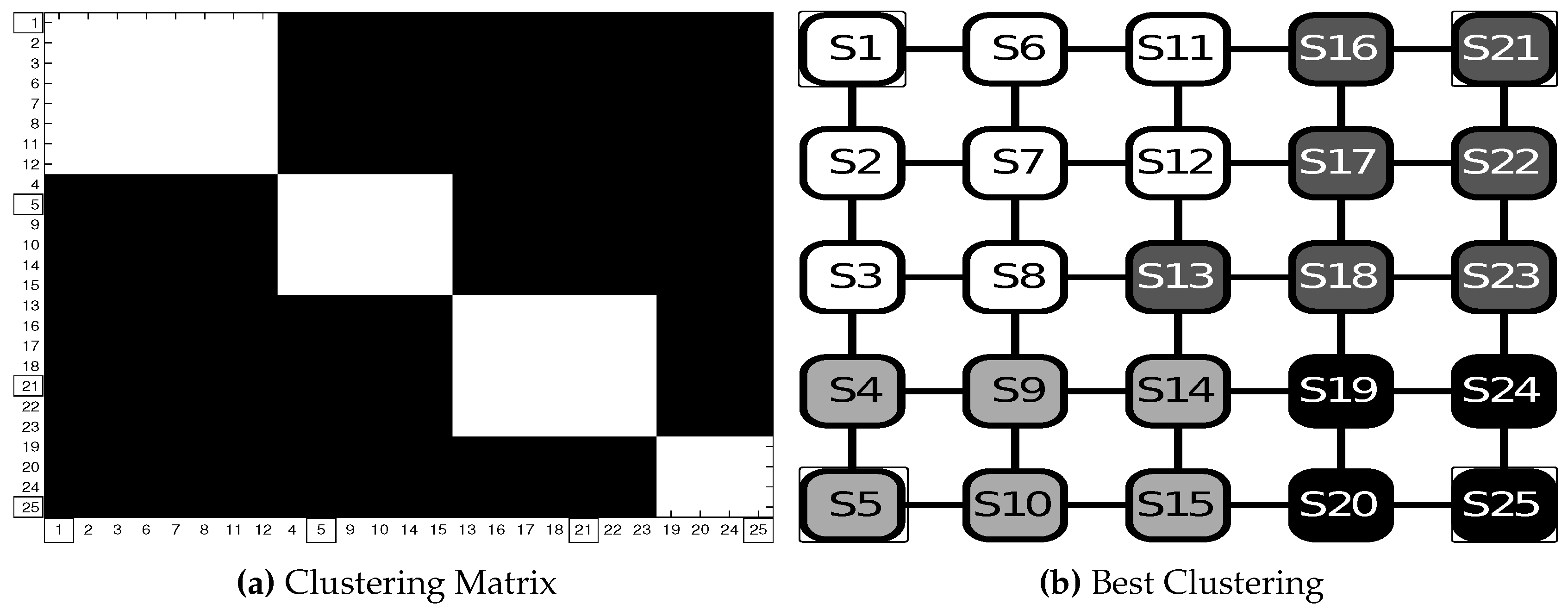
Open space scenario. This scenario is composed of 25 discrete states arranged in a square with all transitions enabled for the neighboring states. In this scenario, no structure restrictions (e.g., bottlenecks) are present. See Figure 3a.

(ii)

Grid world scenario. This scenario consists of an environment of 29 states grouped into four rooms. Here, rooms are groups of states linked together by restrictions (bottlenecks), i.e., states that allow the transition from a room to another (States $S3,S12,S13,S22$). In our scenario, we can identify four rooms: Room 1 (states $S1,S2,S7,S8$), Room 2 ($S4,S5,S6,S9,S10,S11$), Room 3 ($S14,S15,S16,S19,S20,S21,S25,S26,S27$) and Room 4 ($S17,S18,S23,S24,S28,S29$). See Figure 3b.

(iii)

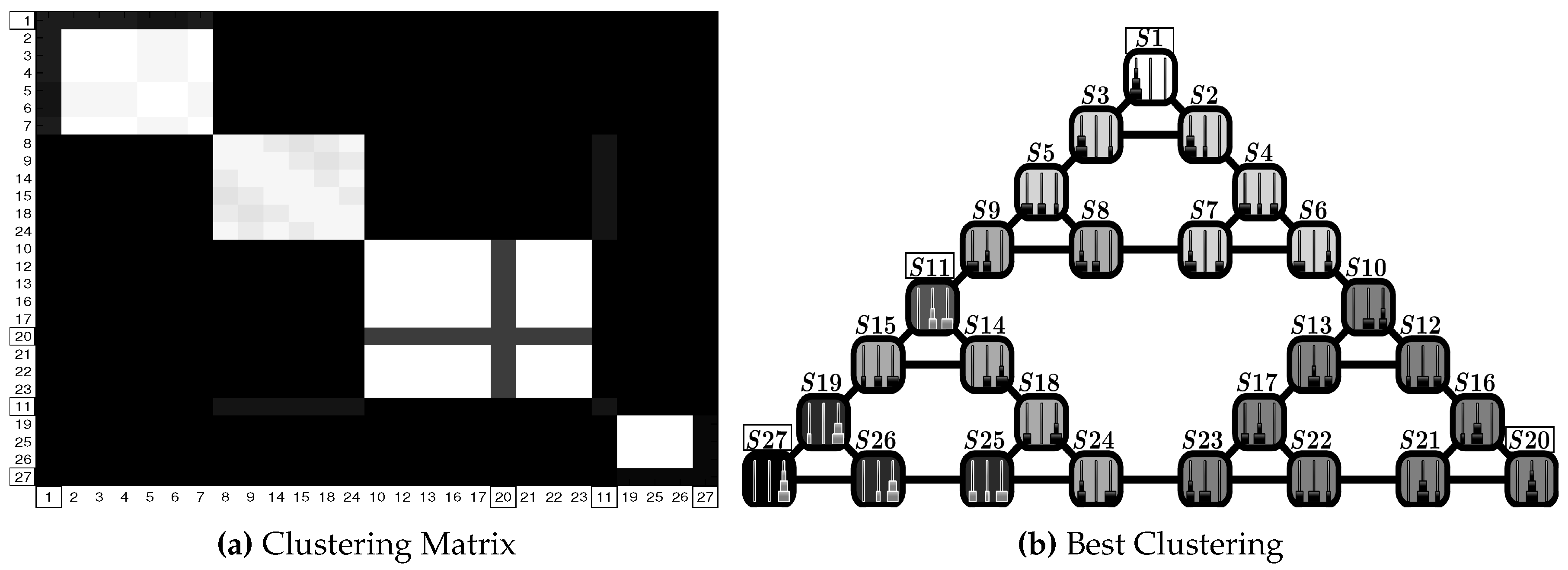
Hanoi Tower scenario. This scenario models a tower of Hanoi (ToH) game of three disks of different sizes that can slide into three rods. Using a well-known mapping [51], the “three pegs-three rods” ToH problem is converted into a path planning problem of 27 states. In this scenario, a recursive community structure can be identified [12], i.e., sets of similar moves separated by bottlenecks represented by different kinds of transitions. In this scenario, it is possible to identify bottlenecks at different hierarchical levels: third order bottlenecks ($S9$–$S11$, $S6$–$S10$ and $S23$–$S24$), second order bottlenecks (e.g., $S3$–$S5$, $S2$–$S4$ and $S7$–$S8$) and first order bottlenecks (e.g., $S1$–$S2$, $S1$–$S3$ and $S2$–$S3$. Transitions among states are shown in Figure 3c.

3.2. Simulations and Results

Our simulations compared the five aforementioned geCRP schemes on all three scenarios, plus two ancillary simulations, for a total of 17 simulations. For each simulation, we performed 25 repetitions (runs) by fixing to 50 the maximum number of iterations for the Gibbs samplings. Results are presented by means of two kinds of graphs:

• The clustering matrix graph illustrates a symmetric matrix whose elements represent the empirical probabilities $P_{C_k}(s_i,s_j)$, $k=1,\cdots ,T$, that two states $s_i$ and $s_j$ belong to the same cluster $C_k$ in the 25 repetitions. The matrix values are shown in gray scale with lighter (darker) colors for higher (lower) frequency to find two states in the same cluster. The size of the clustering matrix for a scenario of N states is $N\times N$. The states are sorted in rows and columns by reflecting the best clustering partition of the 25 repetitions, where by the best clustering, we mean the one that maximize Equation (26) (see below). States within the same cluster follow no particular order. The ordering of the different clusters is assigned with an intuitive criterion: when selecting a geCRP scheme, it is possible to assign to every state an algorithmic probability value computed according to the adopted geCRP scheme. Consequently, we can assign to clusters the mean of the probabilities of the states that belong to them, and then, we can order the clusters as a function of these mean values. Intuitively, clusters that are close in this ordering are clusters containing states with similar probability values. As a consequence, the presence of a “block” in the matrix reveals how frequent a cluster appears in the cluster configurations carried out in the 25 runs;
• The best clustering graph shows the best clustering result found in 25 runs. The best clustering result is acknowledged as the cluster configuration that maximizes the log-likelihood:

  $$\mathcal{L}(C_1,\cdots ,C_T|s_{1:N})=\sum _{k=1}^{T}logp\left(s_{z\left(c_{1:N}\right)=k}\right|z\left(c_{1:N}\right))$$

  (26)

  where $C_1,\cdots ,C_T$ are the clusters and $p\left(s_{z\left(c_{1:N}\right)=k}\right|z\left(c_{1:N}\right))$ is the likelihood of observations defined in Equation (25).

3.3. Results in the Open Space Scenario

In this section, we show the results of five tests, one for each geCRP scheme (from OS1–5), in the open space scenario. Experimental parameters are summed up in

Table 1. Parameter setup for Tests OS1–5 in the open space scenario. geCRP, generative embedded Chinese restaurant process.

Test	OS1	OS2	OS3	OS4	OS5
geCRP scheme	$geCRP/subg/L$	$geCRP/struc/L$	$geCRP/goal/L$	$geCRP/path/L$	$geCRP/multig/L$
α	0.08	0.08	0.008	0.008	0.08
λ	$1\times {10}^{-5}$	$1\times {10}^{-5}$	$1\times {10}^{-4}$	$1\times {10}^{-5}$	0.1
case-specific setup	–	–	$s_g=19$	$s_o=S1$, $s_g=S25$	goals: $S1$, $S21$, $S5$, $S25$

.

In Figure 4, we show the results for the Test OS1 where $geCRP/subg/L$ is employed. Figure 4a,b shows how the states are partitioned as a function of their probability value. The first cluster is constituted by central state $S13$, then the cluster $\{S8,S12,S14,S18\}$ down to the last cluster constituted $\{S1,S5,S21,S25\}$ by states in the corners. In particular, from Figure 4a, the stability of the solutions found in the 25 runs is evident.

In Test OS2, $geCRP/struc/L$ failed to find a stable cluster configuration. In fact, as we mentioned, no bottlenecks are present, so all model values are very close, and consequently, as we expected, a clusterization based on the structure does not make sense. This means that from a structural point of view, either all states belong to the same cluster or all states are different clusters. Figure 5a shows that no stable cluster configuration exists: each state has a considerable probability of falling in a cluster with every state of the environment.

In Test OS3, we search for clusters with $geCRP/goal/L$, where the goal state is $s_g=19$. Results are shown in Figure 6. With the absence of a bottleneck structure, it is evident that the series of radial clustering degrades with the number of transitions toward the goal state. It starts with the first cluster in which the only goal state is present, then the next cluster is formed by the neighboring states $\{S14,S18,S20,S24\}$, and so on, down to the last cluster of more distant states, i.e., $\{S1,S2,S3,S4,S5,S5,S7,S11,S16,S21\}$.

Test OS4 is performed with $geCRP/path/L$, setting $s_o=S1$ as the starting state and $s_g=S25$ as the final state. Figure 7 shows the corresponding clustering results. Clusters are divided into groups with respect to the number of transitions from the starting and final states. Thus, $S1$ and $S25$ are in two separate clusters, then a unique cluster with the set $\{S2,S2,S10\}$, and so on, down to the “peripheral” clusters formed by $\left\{S13\right\}$ and $\{S5,S21\}$.

Figure 8 shows Test OS5 with the results of $geCRP/multig/L$ with goals = $S1$, $S21$ and $S15$ and $S25$. In Figure 8b, it is possible to see four clusters in the best clustering: one for each goal, and a further cluster for states peripheral for the other three ones. In Figure 8a, the clustering matrix, we can notice that this cluster configuration is very stable.

3.4. Results in the Grid World Scenario

In this section, we show the results for six tests in the grid world scenario, GW1–6, in which the ability of the different geCRP schemes is explored (see

Table 2. Parameter setup for Grid World Tests GW1–6 in the grid world scenario.

Test	GW1	GW2	GW3	GW4	GW5	GW6
geCRP scheme	$geCRP/subg/L$	$geCRP/struc/L$	$geCRP/goal/L$	$geCRP/path/L$	$geCRP/multig/L$	$geCRP/multig/L$
α	0.008	0.08	0.008	0.008	0.01	0.01
λ	$1\times {10}^{-3}$	$1\times {10}^{-4}$	$1\times {10}^{-6}$	$1\times {10}^{-7}$	$1\times {10}^{-7}$	$1\times {10}^{-7}$
case-specific	–	–	$s_g=S25$	$s_o=S6$, $s_g=S25$	goals: $S25$, $S1$, $S13$	goals: $S25$, $S1$,
setup						$S13$, $S6$, $S29$

for the experimental parameter set up.)

Figure 9 shows clustering results for the GW1 test with $geCRP/subg/L$. Figure 9b shows the best cluster partition found in the 25 runs. The number of clusters is five: it is possible to note that the least likely states, as the bottleneck states, are put in the same cluster, while the most likely are the ones inside the rooms, near the bottlenecks (see [8]) and are put in the same cluster. Figure 9a shows that another successful solution is to group two clusters together and to obtain four total clusters. Moreover, by changing the scaling parameter (λ) and the concentration parameter (α), it is possible to get a finer partition grouped into smaller clusters.

Figure 10 shows clustering results for the GW2 test, i.e., the application of the $geCRP/struc/L$ scheme. Figure 10b shows the best clustering in the 25 runs. As is appreciable, this scheme was able to cluster the 27 states into four clusters, each one representing a different room. Moreover, in Figure 10a, it is possible to see four blocks, meaning that this configuration is stable with respect to different runs. Note that bottleneck States $S3,S12,S13,S22$ do not always belong to the same room (as expected), but are alternatively assigned to one of the neighboring clusters: for example, $S3$ has equal probability to be assigned to Room 1 (cluster $\{S1,S2,S7,S8\}$) or to Room 2 (cluster $\{S4,S5,S6,S9,S10,S11\}$).

Figure 11 shows clustering results for the GW3 test where $geCRP/goal/L$ is used with $S25$ as the goal state. In Figure 11b, the best cluster configuration is depicted. It is noticeable how clusters form a kind of “gradient field” originating from the goal state and degrading with the length of the path needed to reach the goal. In Figure 11a, it is possible to recognize the 12 clusters found and the stability of the computed solutions.

Figure 12 shows the GW4 test results attained by $geCRP/path/L$ with starting state $s_o=S6$ and final state $s_g=25$. The best cluster in Figure 12b shows how states are divided into groups with respect to the number of transitions from the starting and final states. Figure 12a shows the 12 clusters found and their stability in the set of 25 repetitions.

Figure 13 shows the results for Test GW5 with $geCRP/multig/L$ and goals = $\{S25,S1,S13\}$. In Figure 13b is shown the best clustering. As one can discern, if one of the goals is a bottleneck state, then the scheme produces a unique cluster that merges the two rooms (Rooms 2 and 4, in this case), while Room 1 (where $S1$ is) and Room 2 (where $S25$ is) are clustered apart. $S25$ is here inserted alone in a different cluster. However, it is possible to note from Figure 13a that, often, it is assigned to the same cluster of Room 2. A similar consideration can be done for state $S1$.

Figure 14 shows the GW6 test results for $geCRP/multig/L$ with goals = $\{S25,S1,S13,S6,S29\}$, in which the importance of the generative model in modifying the “information geometry” of the scenario is even more evident. In Figure 14b, the best clustering shows for each goal a cluster formed by neighboring states taking into account the shape of the rooms. In Figure 14a, the five clusters are evident, and it is possible to get that the “central” states of the clusters are very stable, while “frontier” states are possibly assigned to different clusters.

3.5. Results in the Hanoi Tower Scenario

Similarly to the previous scenarios, we show the clustering results for six tests, ToH1–6, performed in the Hanoi Tower scenario by means of the five geCRP schemes proposed (see

Table 3. Parameter set-up for Tower of Hanoi Tests ToH1–6 in the Hanoi Tower scenario.

Test	ToH1	ToH2	ToH3	ToH4	ToH5	ToH6
geCRP scheme	$geCRP/subg/L$	$geCRP/struc/L$	$geCRP/goal/L$	$geCRP/path/L$	$geCRP/multig/L$	$geCRP/multig/L$
α	0.08	0.08	0.008	0.08	0.1	0.1
λ	$1\times {10}^{-5}$	$1\times {10}^{-5}$	$1\times {10}^{-7}$	$1\times {10}^{-8}$	$1\times {10}^{-3}$	$1\times {10}^{-3}$
case-specific	–	–	$s_g=S20$	$s_o=S27$, $s_g=S20$	goals: $S27$, $S20$	goals: $S1$, $S11$,
setup						$S20$, $S27$

for details on parameter set up).

Figure 15 shows the ToH1 test with $geCRP/subg/L$. The states are partitioned into clusters of different probability values. From Figure 15b, notice for instance that vertex states, corresponding to the final configurations of the ToH game, are put in the first cluster $\{S1$, $S20$, $S27\}$, while the second cluster $\{S6,S9,S10,S11,S23,S24\}$ consists of third order bottlenecks. In Figure 15a, it is possible to see both the five clusters that the $geCRP/subg/L$ scheme finds and how stable they are in all 25 runs.

Figure 16 shows the ToH2 test where $geCRP/struc/L$ is applied. Figure 16a shows the best clustering found. The states of the Hanoi Tower scenario are divided into three clusters, each one forming a community structure and separated by third order bottlenecks (e.g., $S23$–$S24$). Figure 16b illustrates that these three clusters are empirically the most probable solution in this scheme.

Figure 17 reports the results for the ToH3 test obtained by means of $geCRP/goal/L$, with the goal state set to $s_g=S20$. In Figure 17b, similarly for the corresponding test in the grid world scenario, it is possible to identify the sequence of clusters arranged in a gradient-like fashion, starting from the goal state, up to the farthest cluster, i.e., the set $\{S1$, $S3$, $S5$, $S9$, $S11$, $S15$, $S19$, $S27\}$. In Figure 17a, the clustering matrix for the 25 repetitions is shown. Note that another possible solution is to group together the last two clusters of the best solutions, $\{S2,S8,S13,S26\}$ and $\{S1,S3,S5,S9,S11,S15,S19,S27\}$.

Figure 18 depicts ToH4 results with $geCRP/path/L$ used as the scheme with starting state $s_o=S27$ and final state $s_g=20$. Figure 18b presents the best clustering solution: clusters are divided into groups with respect to the number of moves necessary to go from the starting to the final state. Thus, we can see that the start and final states belong to two different clusters and are followed by other intermediate clusters with a “central”, more distant cluster composed of the states $S1,S2,S3,S4,S5,S6,S7,S8,S9$. Figure 18a shows the ordered 12 clusters found, and also, in this case, the achieved solutions result in being very stable.

Figure 19 is related to the results of the test ToH5 attained with $geCRP/multig/L$ and the set $\{S27,S20\}$ as goals. Figure 19b shows the best cluster configuration, while from the clustering matrix, in Figure 19a, we can estimate six (symmetric) clusters. In contrast with the $geCRP/path/L$ scheme, here, the multiple goal-sensitive model builds up clusters as a function of the community structure and bottlenecks of first (e.g., $S20$–$S21$), second (e.g., $S21$–$S22$) and third (e.g., $S23$–$S24$) order. That determines substantial differences between the two cluster configurations, though they both have $\{S27,S20\}$ as reference states: $geCRP/path/L$ focuses on the shortest path, while $geCRP/multig/L$ forms two gradient-like cluster sequences centered on the selected goals.

A similar behavior is confirmed in the ToH6 test (Figure 20) performed with $geCRP/multig/L$ with the set $\{S1,S11,S20,S27\}$. Figure 20a,b reports solutions found for this set up: it is possible to notice the clusters arranged in a gradient field fashion induced by the selected goals. It is interesting to notice that the selection of the goal $S11$ breaks the symmetry of the solutions, and the “isolated” goal $S20$ forms with neighboring states a cluster that is similar to a structure-based one.

4. Discussion

We presented a novel nonparametric approach, the generative embedded Chinese restaurant process (geCRP), which essentially creates clusters in data, and thus task decompositions, that can reflect different information measures (encoded as generative embedded kernels). Using different generative embedded kernels within the same nonparametric clustering method, we realized five algorithmic probabilistic models (sub-goal-sensitive, structure-sensitive, goal-sensitive, path-sensitive and multiple-goal-sensitive models), which are able to support a variety of cognitive control tasks, ranging from exploration to the achievement of one or more goals (see Section 2.2.1).

We tested and compared these five models in three scenarios: (1) an open space, an environment without any geometric characteristics, i.e., with no bottlenecks; (2) a grid world, which is an instance of a structured environment with four rooms; and (3) a Hanoi Tower, a classical problem used to investigate human executive function, which has a self-similar state space, i.e., it is composed of small communities that recursively compose other communities with larger sizes.

For each scenario, we compared the planning performance of the (best cluster configurations of the) five models, in a series of tasks that required exploring the environment, to reach a goal from a known or an unknown solution or to reach multiple goals. Our analysis reveals that each of the five models decomposes the task (or finds clusters in the data) in a way that is more appropriate for one of these tasks. Specifically:

• The sub-goal-sensitive model is able to reveal useful sub-goal- or bottleneck-related information (i.e., extract states that can act as useful sub-goals or bottlenecks), if present in the environment. This can be considered a clustering method that is “agnostic” with regard to the specific behavioral goal of the agent, but can be used for planning from any start state to any goal state.
• The structure-sensitive model clusters the environment into coherent geometric partitions or shapes, e.g., rooms in a four-room scenario (grid world). However, in the open space, this method does not find coherent partitions; because every couple of states has the same similarity metric, each clustering experiment produces a different partitioning, due to the stochasticity of Gibbs sampling.
• The goal-sensitive model generates a clustering that groups the states according to a gradient-field that culminates in the goal site and affords effective navigation to a known goal. This method shares some resemblances with value functions that are widely used in reinforcement learning methods, which essentially create gradients to reward locations [6]. Our results indicate that this clustering method is appropriate for planning a path to a known goal location, from any start location.
• The path-sensitive model groups states on the basis of their probability values with respect to both a starting and a goal state, both of which are known a priori. The results indicate that this clustering method is appropriate for planning a path from a known start location to a known goal location.
• The multiple goal-sensitive model groups states in a way that is similar to the goal-sensitive model, but for several (known) goal states. The results show that this clustering method is appropriate when the planning problem includes multiple goal locations. Interestingly, the number and location of goals entail a modification, in an informational sense, of the geometry of the scenario. Consider for example the case of the grid world with three goals, one of which is a bottleneck. Although the scenario is characterized by the presence of four rooms, the model only produces three clusters, thus clustering together two rooms. The dependence of the clustering from the agent’s objectives (here, reaching multiple goal locations) is a hallmark of flexible coding schemes.

Taken together, these results show that the geCRP method can create different clusters that are most effective to address different cognitive control tasks. Key to solving these tasks efficiently is devising a task decomposition that extracts the most relevant structure from the data. A contribution of this paper is showing that such a structure can be formally related to information theoretic and probabilistic measures, such as the conditional or the joint probability between two states, and that these information measures can all be used within the same generative geCRP method to obtain a variety of clusters, each with a different sensitivity to goal, sub-goal, path or other kinds of control-related information. Regardless, it should be pointed out that the introduced definitions of the algorithmic probabilities hinge on the assumption that transitions between states need to be symmetric (this is especially true for Equation (8)). A potential extension of this work would be aimed to reconsider those definitions in the case of asymmetric transitions and to study their feasible applications.

Of note, the generative kernels used in this work can have different forms: they can depend on the distance between probability values or, as in the case of the structure-sensitive control task, they are functions of joint probabilities. This requirement motivates our choice of the geCRP over other related schemas (e.g., ddCRP), which do not have this flexibility. Many other generative kernels can be designed by starting from various probability distributions, in order to address particular problems. Identifying the best kernels for different families of problems is an open objective for future research.

It can also be noted that the probability values computed by any of the five geCRP schemes might be useful per se during (for example) path planning, rather than just for clustering; see [11] for an example. However, here, we are interested in clustering methods that afford dimensionality reduction (as the number of cluster is smaller than the number of states) and ultimately efficiency in representation, learning and inference. For example, the clusters emerging using the geCRP schemes might be used by hierarchical algorithms [52,53] that represent information at different levels of granularity at the different hierarchical layers, thus permitting one to plan in terms of macro-actions and not elementary actions. Here, a key thing to note is that besides extracting a set of clusters, our procedure also distinguishes them for their relative informational value (e.g., in the figures, the more probable states are colored darker). In principle, this information can be exploited (for example) by planning algorithms that “climb” a probability gradient. Studying whether the clusters studied here can improve hierarchical learning and inference schemes is an important objective for future research.

5. Conclusions

It is well known in fields like AI and RL that finding appropriate task decomposition is key to solving complex problems [4,5,6]. The contribution of this paper to the literature is identifying a mapping between different control problems and corresponding information measures, all of which can be used within a unitary method to derive task-relevant decompositions or clusters. Indeed, the results we report show that, first, different control problems can benefit from different task decompositions and, second, that it is possible to characterize these decompositions in terms of a unitary computational scheme (geCRP), where different well-known information measures are used as kernels.

From a cognitive perspective, the information measures presented here might be used by the brain to efficiently represent and solve different classes of control problems. Analogous to the way the visual system is hypothesized to be sensitive to the natural statistics of visual scenes, some brain areas or networks might be sensitive to the natural statistics of control tasks. A plausible neuronal substrate for the acquisition of task-relevant representations is the prefrontal cortex (PFC), which has been consistently linked to both cognitive control and flexible coding schemes, in the sense that PFC neurons can be broadly tuned to multiple attributes, and adapt to the attributes that are more relevant to the task at hand [13,17]. The contribution of this article to this body of evidence is showing that task representations that afford various forms of cognitive control can be characterized in terms of well-known information measures, which can have a plausible neuronal implementation [3]. In principle, the method illustrated here can be used to identify neuronal equivalents of the geCRP clusters in the PFC or other brain areas.

An open problem in this field is how task-relevant representations might be created in the first place, with alternative theories that link to statistical learning in the PFC proper or assign a role for the hippocampus in rapidly creating these clusters (or schemas [54]) and transferring them to cortical structures [18,55,56]. Either way, it is unclear whether and how the brain addresses the computational complexity of the learning and inference problems studied here. For example, a growing body of evidence supports the view that the PFC can perform nonparametric statistical learning and inference. Nevertheless, given the computational complexity of full Bayesian inference processes, it is still unclear whether specific approximations or heuristics might be used [17,57,58,59].

Even if one assumes that the PFC is able to learn different clusterings or task representations, another open problem is understanding how it might flexibly select among them depending on the task at hand. Various studies suggest that the PFC can rapidly shape its codes through learning, even with very few examples, and rapidly modify them when the task demands change; in this way, the PFC might support behavioral flexibility and rapid rule learning. However, the computational principles underlying these abilities are disputed [60,61]. It is appealing to speculate that the PFC might implement a unitary statistical process (analogous to geCRP) that is however able to differentiate its output (and thus support various cognitive control tasks) by flexibly selecting among different task representations or, in terms of our approach, by selecting the best kernel depending on the task at hand. In principle, the PFC might learn over time the best kernel to use for a given task in the same way it learns the best rule or task set to use [17,58,62], and this mechanism might provide the necessary flexibility to face a number of different problems. A prediction stemming from this hypothesis is that PFC neurons would be sensitive to different information measures (equivalent to the clusters used here) depending on the task at hand. This hypothesis, however, remains to be assessed in future studies.

References

1. Olshausen, B.A.; Field, D.J. Emergence of simple-cell receptive field properties by learning a sparse code for natural images. Nature 1996, 381, 607–609. [Google Scholar] [CrossRef] [PubMed]
2. Simoncelli, E.P.; Olshausen, B.A. Natural image statistics and neural representation. Annu. Rev. Neurosci. 2001, 24, 1193–1216. [Google Scholar] [CrossRef] [PubMed]
3. Friston, K. The free-energy principle: A unified brain theory? Nat. Rev. Neurosci. 2010, 11, 127–138. [Google Scholar] [CrossRef] [PubMed]
4. Botvinick, M.; Weinstein, A.; Solway, A.; Barto, A. Reinforcement learning, efficient coding, and the statistics of natural tasks. Curr. Opin. Behav. Sci. 2015, 5, 71–77. [Google Scholar] [CrossRef]
5. Russell, S.; Norvig, P. Artificial Intelligence: A Modern Approach, 3rd ed.; Prentice Hall: Upper Saddle River, NJ, USA, 2009. [Google Scholar]
6. Sutton, R.; Barto, A. Reinforcement Learning: An Introduction; MIT Press: Cambridge, MA, USA, 1998. [Google Scholar]
7. Mnih, V.; Kavukcuoglu, K.; Silver, D.; Rusu, A.A.; Veness, J.; Bellemare, M.G.; Graves, A.; Riedmiller, M.; Fidjeland, A.K.; Ostrovski, G.; et al. Human-level control through deep reinforcement learning. Nature 2015, 518, 529–533. [Google Scholar] [CrossRef] [PubMed]
8. Van Dijk, S.G.; Polani, D. Grounding sub-goals in information transitions. In Proceedings of the 2011 IEEE Symposium on Adaptive Dynamic Programming and Reinforcement Learning (ADPRL), Paris, France, 11–15 April 2011; IEEE: Piscataway, NJ, USA, 2011; pp. 105–111. [Google Scholar]
9. Van Dijk, S.G.; Polani, D.; Nehaniv, C.L. Hierarchical behaviours: Getting the most bang for your bit. In Advances in Artificial Life. Darwin Meets von Neumann; Springer: Berlin/Heidelberg, Germany, 2011; pp. 342–349. [Google Scholar]
10. Van Dijk, S.; Polani, D. Informational Constraints-Driven Organization in Goal-Directed Behavior. Adv. Complex Syst. 2013, 16. [Google Scholar] [CrossRef]
11. Maisto, D.; Donnarumma, F.; Pezzulo, G. Divide et impera: Subgoaling reduces the complexity of probabilistic inference and problem solving. J. R. Soc. Interface 2015, 12. [Google Scholar] [CrossRef] [PubMed]
12. Solway, A.; Diuk, C.; Cordova, N.; Yee, D.; Barto, A.G.; Niv, Y.; Botvinick, M.M. Optimal behavioral hierarchy. PLoS Comput. Biol. 2014, 10, e1003779. [Google Scholar] [CrossRef] [PubMed]
13. Rigotti, M.; Barak, O.; Warden, M.R.; Wang, X.J.; Daw, N.D.; Miller, E.K.; Fusi, S. The importance of mixed selectivity in complex cognitive tasks. Nature 2013, 497, 585–590. [Google Scholar] [CrossRef] [PubMed]
14. Genovesio, A.; Tsujimoto, S.; Wise, S.P. Encoding goals but not abstract magnitude in the primate prefrontal cortex. Neuron 2012, 74, 656–662. [Google Scholar] [CrossRef] [PubMed]
15. Pezzulo, G.; Castelfranchi, C. Thinking as the Control of Imagination: A Conceptual Framework for Goal-Directed Systems. Psychol. Res. PRPF 2009, 73, 559–577. [Google Scholar] [CrossRef] [PubMed]
16. Pezzulo, G.; Rigoli, F.; Friston, K. Active Inference, homeostatic regulation and adaptive behavioural control. Prog. Neurobiol. 2015, 134, 17–35. [Google Scholar] [CrossRef] [PubMed]
17. Stoianov, I.; Genovesio, A.; Pezzulo, G. Prefrontal goal-codes emerge as latent states in probabilistic value learning. J. Cogn. Neurosci. 2015, 28, 140–157. [Google Scholar] [CrossRef] [PubMed]
18. Verschure, P.F.M.J.; Pennartz, C.M.A.; Pezzulo, G. The why, what, where, when and how of goal-directed choice: Neuronal and computational principles. Philos. Trans. R. Soc. B 2014, 369. [Google Scholar] [CrossRef] [PubMed]
19. Pitman, J. Combinatorial Stochastic Processes; Picard, J., Ed.; Springer: Berlin/Heidelberg, Germany, 2006. [Google Scholar]
20. Blei, D.M.; Frazier, P.I. Distance dependent Chinese restaurant processes. J. Mach. Learn. Res. 2011, 12, 2461–2488. [Google Scholar]
21. Murphy, K.P. Machine Learning: A Probabilistic Perspective; MIT Press: Cambridge, MA, USA, 2012; p. 15. [Google Scholar]
22. Therrien, C.W. Decision Estimation and Classification: An Introduction to Pattern Recognition and Related Topics; Wiley: Hoboken, NJ, USA, 1989. [Google Scholar]
23. Ferguson, T.S. A Bayesian analysis of some nonparametric problems. Ann. Stat. 1973, 1, 209–230. [Google Scholar] [CrossRef]
24. Dahl, D.B. Distance-based probability distribution for set partitions with applications to Bayesian nonparametrics. In JSM Proceedings, Section on Bayesian Statistical Science, Washington, DC, USA, 30 July–6 August 2009.
25. Ahmed, A.; Xing, E. Dynamic Non-Parametric Mixture Models and the Recurrent Chinese Restaurant Process: With Applications to Evolutionary Clustering. In Proceedings of the 2008 SIAM International Conference on Data Mining, Atlanta, GA, USA, 24–26 April 2008; pp. 219–230.
26. Zhu, X.; Ghahramani, Z.; Lafferty, J. Time-Sensitive Dirichlet Process Mixture Models; Technical Report CMU-CALD-05-104; Carnegie Mellon University: Pittsburgh, PA, USA, May 2005. [Google Scholar]
27. Rasmussen, C.E.; Ghahramani, Z. Infinite mixtures of Gaussian process experts. Adv. Neural Inf. Process. Syst. 2002, 2, 881–888. [Google Scholar]
28. Haussler, D. Convolution Kernels on Discrete Structures; Technical Report UCSC-CRL-99-10; University of California at Santa Cruz: Santa Cruz, CA, USA, July 1999. [Google Scholar]
29. Jaakkola, T.; Haussler, D. Exploiting generative models in discriminative classifiers. In Advances in Neural Information Processing Systems; MIT Press: Cambridge, MA, USA, 1999; pp. 487–493. [Google Scholar]
30. Shawe-Taylor, J.; Cristianini, N. Kernel Methods for Pattern Analysis; Cambridge university Press: Cambridge, UK, 2004. [Google Scholar]
31. Brodersen, K.H.; Schofield, T.M.; Leff, A.P.; Ong, C.S.; Lomakina, E.I.; Buhmann, J.M.; Stephan, K.E. Generative embedding for model-based classification of fMRI data. PLoS Comput. Biol. 2011, 7, e1002079. [Google Scholar] [CrossRef] [PubMed] [Green Version]
32. Li, M.; Vitányi, P.M. An Introduction to Kolmogorov Complexity and Its Applications; Springer: Berlin/Heidelberg, Germany, 2009. [Google Scholar]
33. Solomonoff, R.J. A formal theory of inductive inference. Part I. Inf. Control 1964, 7, 1–22. [Google Scholar] [CrossRef]
34. Solomonoff, R.J. A formal theory of inductive inference. Part II. Inf. Control 1964, 7, 224–254. [Google Scholar] [CrossRef]
35. Solomonoff, R.J. Complexity-based induction systems: Comparisons and convergence theorems. IEEE Trans. Inf. Theory 1978, 24, 422–432. [Google Scholar] [CrossRef]
36. Hutter, M. Universal Artificial Intelligence: Sequential Decisions based on Algorithmic Probability; Springer: Berlin/Heidelberg, Germany, 2005. [Google Scholar]
37. Zvonkin, A.K.; Levin, L.A. The complexity of finite objects and the development of the concepts of information and randomness by means of the theory of algorithms. Russ. Math. Surv. 1970, 25, 83–124. [Google Scholar] [CrossRef]
38. Van Dijk, S.G.; Polani, D. Informational constraints-driven organization in goal-directed behavior. Adv. Complex Syst. 2013, 16, 1350016. [Google Scholar] [CrossRef]
39. Newell, A.; Simon, H.A. Human Problem Solving; Prentice Hall: Upper Saddle River, NJ, USA, 1972. [Google Scholar]
40. Schölkopf, B.; Tsuda, K.; Vert, J.P. Kernel Methods in Computational Biology; MIT Press: Cambridge, MA, USA, 2004. [Google Scholar]
41. Ruiz, A.; López-de-Teruel, P.E. Nonlinear kernel-based statistical pattern analysis. IEEE Trans. Neural Netw. 2001, 12, 16–32. [Google Scholar] [CrossRef] [PubMed]
42. Storn, R.; Price, K. Differential evolution—A simple and efficient heuristic for global optimization over continuous spaces. J. Glob. Optim. 1997, 11, 341–359. [Google Scholar] [CrossRef]
43. Geman, S.; Geman, D. Stochastic relaxation, Gibbs distributions, and the Bayesian restoration of images. IEEE Trans. Pattern Anal. Mach. Intell. 1984, PAMI-6, 721–741. [Google Scholar] [CrossRef]
44. Robert, C.; Casella, G. Monte Carlo Statistical Methods; Springer: Berlin/Heidelberg, Germany, 2013. [Google Scholar]
45. Neal, R.M. Markov chain sampling methods for Dirichlet process mixture models. J. Comput. Graph. Stat. 2000, 9, 249–265. [Google Scholar]
46. Anderson, J.R. The adaptive nature of human categorization. Psychol. Rev. 1991, 98, 409–429. [Google Scholar] [CrossRef]
47. Borgatti, S.P. Centrality and network flow. Soc. Netw. 2005, 27, 55–71. [Google Scholar] [CrossRef]
48. Tishby, N.; Polani, D. Information Theory of Decisions and Actions. In Perception-Action Cycle; Springer: Berlin/Heidelberg, Germany, 2011; pp. 601–636. [Google Scholar]
49. Barrat, A.; Barthelemy, M.; Vespignani, A. Dynamical Processes on Complex Networks; Cambridge University Press: Cambridge, UK, 2008. [Google Scholar]
50. Barto, A.G.; Mahadevan, S. Recent advances in hierarchical reinforcement learning. Discret. Event Dyn. Syst. 2003, 13, 41–77. [Google Scholar] [CrossRef]
51. Nilsson, N.J. Problem-Solving Methods in Artificial Intelligence; McGraw-Hill: New York, NY, USA, 1971. [Google Scholar]
52. Botvinick, M.M. Hierarchical models of behavior and prefrontal function. Trends Cogn. Sci. 2008, 12, 201–208. [Google Scholar] [CrossRef] [PubMed]
53. Kiebel, S.J.; Daunizeau, J.; Friston, K.J. A hierarchy of time-scales and the brain. PLoS Comput. Biol. 2008, 4, e1000209. [Google Scholar] [CrossRef] [PubMed]
54. Tse, D.; Langston, R.F.; Kakeyama, M.; Bethus, I.; Spooner, P.A.; Wood, E.R.; Witter, M.P.; Morris, R.G.M. Schemas and memory consolidation. Science 2007, 316, 76–82. [Google Scholar] [CrossRef] [PubMed]
55. Pezzulo, G.; van der Meer, M.A.A.; Lansink, C.S.; Pennartz, C.M.A. Internally generated sequences in learning and executing goal-directed behavior. Trends Cogn. Sci. 2014, 18, 647–657. [Google Scholar] [CrossRef] [PubMed]
56. McClelland, J.L.; McNaughton, B.L.; O’Reilly, R.C. Why there are complementary learning systems in the hippocampus and neocortex: Insights from the successes and failures of connectionist models of learning and memory. Psychol. Rev. 1995, 102, 419–457. [Google Scholar] [CrossRef] [PubMed]
57. Collins, A.; Koechlin, E. Reasoning, learning, and creativity: Frontal lobe function and human decision-making. PLoS Biol. 2012, 10, e1001293. [Google Scholar] [CrossRef] [PubMed]
58. Donoso, M.; Collins, A.G.; Koechlin, E. Foundations of human reasoning in the prefrontal cortex. Science 2014, 344, 1481–1486. [Google Scholar] [CrossRef] [PubMed]
59. Schapiro, A.C.; Rogers, T.T.; Cordova, N.I.; Turk-Browne, N.B.; Botvinick, M.M. Neural representations of events arise from temporal community structure. Nat. Neurosci. 2013, 16, 486–492. [Google Scholar] [CrossRef] [PubMed]
60. Duncan, J. The multiple-demand (MD) system of the primate brain: Mental programs for intelligent behaviour. Trends Cogn. Sci. 2010, 14, 172–179. [Google Scholar] [CrossRef] [PubMed]
61. Passingham, R.E.; Wise, S.P. The Neurobiology of the Prefrontal Cortex: Anatomy, Evolution, and the Origin of Insight; Oxford University Press: Oxford, UK, 2012. [Google Scholar]
62. Donnarumma, F.; Prevete, R.; Chersi, F.; Pezzulo, G. A Programmer-Interpreter Neural Network Architecture for Prefrontal Cognitive Control. Int. J. Neural Syst. 2015, 25, 1550017. [Google Scholar] [CrossRef] [PubMed]
Figure 1. Schematization of the generative embedded Chinese restaurant process. A generative embedded Chinese restaurant process (geCRP) can be viewed as the composition of three different modules. Initially, in Stage 1, a probabilistic model M = ( S , P M ) of the problem at hand has to be defined. M is a probability space where P M is a distribution on the space of events coinciding with the subsets of the problem state space. P M acts as an embedding function that projects (collections of) states in [ 0 , 1 ] . To this aim, any probabilistic framework can be adopted. Here, we adopt a methodology of information theory, the algorithmic probability theory, to construct different distributions, as detailed in Section 2.2.1. Thereafter, in Stage 2, a generative embedded kernel K M : S × S R + is defined that represents a similarity metric and determines a generative score space. This stage is described in Equation (3) and can be thought of as being split into two steps: first, the introduction of a kernel function K : P M ( F ) × P M ( F ) R + by choosing, according to the characteristics of the problem, among those ones of common use (Section 2.2.2); second, the composition of K with the function P M × P M , whose domain is the Cartesian product S × S of the space of states S with itself. In the last stage, Stage 3, the generative embedded kernel is used in a Gibbs sampling scheme (Section 2.2.3) to figure out the cluster partitioning that best explains the observations. The clusters can then be visualized and interpreted according to the generative model adopted in Stage 1.
Entropy 18 00061 g001
Figure 2. Effects of adding/removing a link in the customer link and table assignment representations. Illustration of the potential effects on cluster configurations considered by the Gibbs sampler when adding/removing a link between two customers, in the customer link (left side) and table assignment (right side) representations. When the gray link is removed, it could leave the cluster configuration unaltered (the first two examples from the top) or separate a cluster into two (the example down in the figure). When it is added, it could leave the clustering (the first two examples) or it might merge two distinct clusters into one (the last example).
Entropy 18 00061 g002
Figure 3. 2D discrete scenarios used in the experimental analysis. (a) Open space, a scenario without restrictions and bottlenecks; (b) grid world, four different groups of states linked together by four bottlenecks; (c) Hanoi Tower, a model of the tower of Hanoi game in the configuration of three disks and three rods.
Entropy 18 00061 g003
Figure 4. Test OS1: g e C R P / s u b g / L results in the open space scenario (rectangles highlight the first cluster of sub-goals { S 13 } ). (a) Clustering matrix; (b) best clustering. See Table 1 for the parameters and the text for details.
Entropy 18 00061 g004
Figure 5. Test OS2: g e C R P / s t r u c / L results in the open space scenario. (a) Clustering matrix; (b) best clustering. See Table 1 for the parameters and the text for details.
Entropy 18 00061 g005
Figure 6. Test OS3: g e C R P / g o a l / L results in the open space scenario ( s g = S 19 , highlighted with rectangles in both panels). (a) Clustering matrix; (b) best clustering. See Table 1 for the parameters and the text for details.
Entropy 18 00061 g006
Figure 7. Test OS4: g e C R P / p a t h / L results in the open space scenario ( s o = S 1 , s g = S 25 , highlighted with rectangles in both panels). (a) Clustering matrix; (b) best clustering. See Table 1 for the parameters and the text for details.
Entropy 18 00061 g007
Figure 8. Test OS5: g e C R P / m u l t i g / L on the open space scenario(goals = { S 1 , S 21 , S 5 , S 25 } , highlighted with rectangles in both panels). (a) Clustering matrix; (b) best clustering. See Table 1 for the parameters and the text for details.
Entropy 18 00061 g008
Figure 9. Test GW1: g e C R P / s u b g / L results in the grid world scenario (rectangles highlight the first sub-goal cluster { S 10 , S 15 , S 20 , S 21 , S 25 } ). (a) Clustering matrix; (b) best clustering. See Table 2 for the parameters and the text for details.
Entropy 18 00061 g009
Figure 10. Test GW2: g e C R P / s t r u c / L results in the grid world scenario (rectangles highlight bottlenecks S 3 , S 12 , S 13 , S 22 ). (a) Clustering matrix; (b) best clustering. See Table 2 for the parameters and the text for details.
Entropy 18 00061 g010
Figure 11. Test GW3: g e C R P / g o a l / L results in the grid world scenario ( s g = S 25 . highlighted with rectangles in both panels). (a) Clustering matrix; (b) best clustering. See Table 2 for the parameters and the text for details.
Entropy 18 00061 g011
Figure 12. Test GW4: g e C R P / p a t h / L results in the grid world scenario ( s o = S 6 , s g = S 25 , highlighted with rectangles in both panels). (a) Clustering matrix; (b) best clustering. See Table 2 for the parameters and the text for details.
Entropy 18 00061 g012
Figure 13. Test GW5: g e C R P / m u l t i g / L in the grid world scenario (goals = { S 25 , S 1 , S 13 } , highlighted with rectangles in both panels). (a) Clustering matrix; (b) best clustering. See Table 2 for the parameters and the text for details.
Entropy 18 00061 g013
Figure 14. Test GW6: g e C R P / m u l t i g / L in the grid world scenario (goals = { S 25 , S 1 , S 13 , S 6 , S 29 } , highlighted with rectangles in both panels). (a) Clustering matrix; (b) best clustering. See Table 2 for the parameters and the text for details.
Entropy 18 00061 g014
Figure 15. Test ToH1: g e C R P / s u b g / L results in the Hanoi Tower scenario (rectangles highlight the first sub-goal cluster { S 2 , S 3 , S 16 , S 19 , S 21 , S 26 } ). (a) Clustering matrix; (b) best clustering. See Table 3 for the parameters and the text for details.
Entropy 18 00061 g015
Figure 16. Test ToH2: g e C R P / s t r u c / L results in the Hanoi Tower scenario (rectangles highlight third order bottlenecks). (a) Clustering matrix; (b) best clustering. See Table 3 for the parameters and the text for details.
Entropy 18 00061 g016
Figure 17. Test ToH3: g e C R P / g o a l / L results in the Hanoi Tower scenario ( s g = S 20 , highlighted with rectangles). (a) Clustering matrix; (b) best clustering. See Table 3 for the parameters and the text for details.
Entropy 18 00061 g017
Figure 18. Test ToH4: g e C R P / p a t h / L results in the Hanoi Tower scenario ( s o = S 27 , s g = S 20 , highlighted with rectangles). (a) Clustering matrix; (b) best clustering. See Table 3 for the parameters and the text for details.
Entropy 18 00061 g018
Figure 19. Test ToH5: g e C R P / m u l t i g / L results in the grid world scenario (goals = { S 27 , S 20 } , highlighted with rectangles). (a) Clustering matrix; (b) best clustering. See Table 3 for the parameters and the text for details.
Entropy 18 00061 g019
Figure 20. Test ToH6: g e C R P / m u l t i g / L in the Hanoi Tower scenario (goals = { S 1 , S 11 , S 20 , S 27 } , highlighted with rectangles). (a) Clustering matrix; (b) best clustering. See Table 3 for the parameters and the text for details.
Entropy 18 00061 g020