Entropy Generation on MHD Casson Nanofluid Flow over a Porous Stretching/Shrinking Surface

Abstract

In this article, entropy generation on MHD Casson nanofluid over a porous Stretching/Shrinking surface has been investigated. The influences of nonlinear thermal radiation and chemical reaction have also taken into account. The governing Casson nanofluid flow problem consists of momentum equation, energy equation and nanoparticle concentration. Similarity transformation variables have been used to transform the governing coupled partial differential equations into ordinary differential equations. The resulting highly nonlinear coupled ordinary differential equations have been solved numerically with the help of Successive linearization method (SLM) and Chebyshev spectral collocation method. The impacts of various pertinent parameters of interest are discussed for velocity profile, temperature profile, concentration profile and entropy profile. The expression for local Nusselt number and local Sherwood number are also analyzed and discussed with the help of tables. Furthermore, comparison with the existing is also made as a special case of our study.

1. Introduction

Nanofluid is a fluid that is generated by a suspension of solid particles with the dimensions less than 100 nm in fluids. Basically, Nanofluid is a nano-scale colloidal suspension containing condensed nanomaterials. Choi [1] was the first who describe the combination of nanoparticles and base fluid and subsequently termed as nanofluid. In fact, it has two phase system with one phase (liquid phase) and another (solid phase). It can be found to exhibit enlarged thermophysical effects like thermal diffusivity, viscosity, and thermal conductivity compared to those of base liquids such as water, oil and ethylene glycol mixture, etc. It also has many diverse assets in an industrial application, for instance, fuel cell, biomedicine, nuclear reactors and transportation. The performance of heat transfer flow problems in nanofluid has been discussed by Xuan and Li [2] for the assumption of turbulent flow conditions. The declaration of their experimental results emphasized that Nusselt number of nanofluid and convective heat transfer coefficient is enhanced by increasing the Reynolds number and volume fraction of nanoparticles. Khalili [3] solved the model of unsteady convective heat transfer of nanofluid over a stretching wall numerically. In addition, Xiao et al. [4,5] developed a novel form of thermal conductivity of nanofluid with Brownian motion effect and heat transfer of nanofluid by the convection in a pool. He solved both models by a novel technique named as Fractal method and concluded some important results. Natural convection heat transfer inside circular enclosures filled with Alumina nanofluid and heated from below or above has been reported by Ali et al. [6,7]. Nanofluid impingement jet heat transfer and its effect on cooling of a circular dick were studied by Zeitoun and Ali [8,9]. Consequently, a number of review articles with the association of nano fluid performance have been investigated by various researchers [10,11,12].

The fluid flow over stretching surfaces has many important applications in engineering systems, such as metal spinning, drawing on plastic films, the continuous casting of metals, glass blowing and spinning of fibers. All the above-mentioned applications have involved some aspects of flow over stretching sheet, like stagnation point flow over stretching sheet [13,14], Magnetohydrodynamics (MHD) free convection flow with heat transfer [15,16,17] and so on. Moreover, stretching sheet with a porous medium also has received great attention from researchers in the last few years. Hamad and Ferdous [18] examined nanofluid with internal heat generation/absorption and suction/blowing for boundary layer stagnation-point flow over a stretching sheet in a porous medium. Copper–water and silver–water Nanofluid flow over a stretching sheet through a porous medium has been analyzed by Kameshwaran et al. [19].

Magnetic nanofluid is a colloidal suspension of carrier liquid and magnetic nanoparticles. MHD was initially tested in geophysical and astrophysical problems. In recent years, MHD has received significant attention due to its various applications in engineering and petroleum industries. Magnetic nanofluid is also one of them and the main objective of this research area is that fluid flow and heat transfer can be controlled by external magnetic field. Effect of magnetic field on nanofluid with different geometries has been investigated by several researchers. For instance, Rashidi et al. [20] studied buoyancy effect on MHD flow of nanofluid over stretching sheet in the presence of thermal radiation while Sheikholeslami et al. [21] discussed flow and heat transfer in a semi-annulus enclosure in the existence of magnetic and thermal radiation. Moreover, Chamkha [22] reported that MHD flow of uniformly stretching vertical permeable surface in the presence of a chemical reaction and heat generation.

The entropy generation is relaxed in all the studies mentioned above which motivates the current research. Although several models have been proposed to describe MHD effect on stretching surface with various types of fluids but their full potential has not been exploited yet and much work needs to be done. For instance, industrial sectors heating and cooling is important in many aspects including transportation, energy, and electronic devices. Moreover, heat transfer and magnetic effect on biofluids are also great interest, particularly in a physiological system. The main concern in the present analysis is to better understanding about the minimization or entropy generation on heat transfer process. Entropy generation can be expressed as various thermal systems are subjected to irreversibility phenomena and are connected to viscous dissipation, magnetic field and heat and mass transfer. Entropy generation clarifies energy losses in a system evidently in many energy-related applications such as cooling of modern electronic devices or system, geothermal energy systems, etc. Consequently, entropy is a measure of the number of specific ways in which a measure of progressing towards thermodynamics equilibrium. Bejan [23] originally formulated the analysis of entropy generation. Abolbashari et al. [24] have investigated analytically the fluid flow with heat and mass transfer and entropy generation for the steady laminar non-Newtonian nanofluid induced by stretching sheet in the presence of velocity slip and convective surface boundary condition. Few more attempts are taken into account of entropy generation on nanofluid with stretching surface with different geometry [25,26,27,28,29].

In view of the above literature and by realizing the growing need of entropy minimization, the present study brings to its fold many previous studies as particular cases. One of more significance of the current study is the solution of MHD Casson Nanofluid model using a numerical technique, such as Successive Linearization method (SLM) and Chebyshev spectral collocation method. The solution methods for the coupled nonlinear ordinary differential equations are quite interesting. The solution is based upon a choice of a function satisfying the boundary condition and the unknown functions are obtained by iteratively solving the linearized version of the governing equation. Numerical solutions of a temperature profile, concentration profile, entropy generation and velocity profile are computed and demonstrated graphically and mathematically. The obtained results reveal the characteristics of Casson nanofluid and entropy generation. This paper is summarized as follows: after the introduction in Section 1, Section 2 characterizes the mathematical formulation of the governing flow problem, Section 3 shows some important formula of local Nusselt number and local Sherwood number, Section 4 interprets the solution methodology of the problem and Section 5 illustrates the mathematical modeling of entropy generation, while Section 6 and Section 7 are devoted to numerical results and conclusions, respectively.

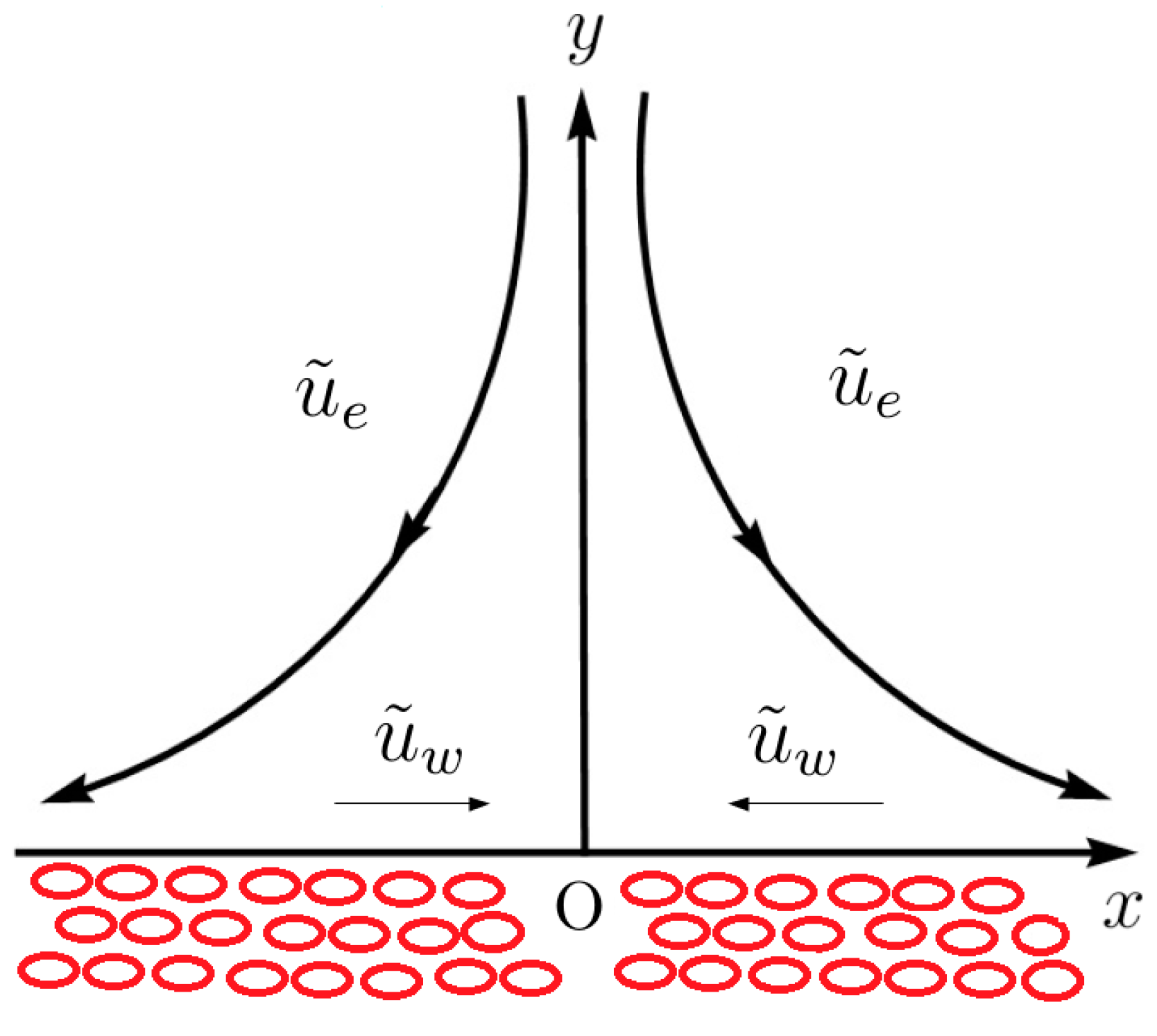
2. Mathematical Formulation

Consider the MHD boundary layer flow over a porous stretching surface near a stagnation point at$y=0$. The MHD flow occurs in the domain at $y>0.$ The fluid is electrically conducting by an external magnetic field while the induced magnetic is assumed to be negligible (or zero). Cartesian coordinate is chosen in a way such that x-axis is considered along the direction of the sheet whereas is y-axis considered along normal to it (see Figure 1). Suppose that $C_w$ be the nano particle fraction at the sheet while the temperature and nano particle fraction at infinity is $T_{\infty }$and$C_{\infty }$, respectively. The velocity of the sheet is considered along x-axis, ${\tilde{u}}_w=ax.$

The rheological equation of state for an isotropic and incompressible Casson fluid is

$${\tau }_{\mathit{i}\mathit{j}}=\{\begin{array}{c}\mathbf{2}{\mathit{e}}_{\mathit{i}\mathit{j}}\left({\mu }_{\mathit{b}}+\frac{{\mathit{P}}_{\mathit{y}}}{\sqrt{\mathbf{2}\Pi }}\right), \mathbf{\Pi }>{\Pi }_{\mathit{C}}, \\ \mathbf{2}{\mathit{e}}_{\mathit{i}\mathit{j}}\left({\mu }_{\mathit{b}}+\frac{{\mathit{P}}_{\mathit{y}}}{\sqrt{\mathbf{2}{\Pi }_{\mathit{c}}}}\right), \mathbf{\Pi }<{\Pi }_{\mathit{C}},\end{array}$$

(1)

where $e_{ij}$ is the component of the deformation rate, $\mathsf{\Pi }$ is the product of the deformation rate and ${\mathsf{\Pi }}_C$ is the critical value of the product based. The governing equations of Casson nanofluid model can be written as

$$\frac{\partial \tilde{u}}{\partial x}+\frac{\partial \tilde{v}}{\partial y}=0,$$

(2)

$$\tilde{u}\frac{\partial \tilde{u}}{\partial x}+\tilde{v}\frac{\partial \tilde{v}}{\partial y}=\nu \left(1+\frac{1}{\mathsf{\beta }}\right)\frac{{\partial }^2\tilde{u}}{\partial y^2}+{\tilde{u}}_e\frac{d{\tilde{u}}_e}{dx}+\frac{\mathsf{\nu }\left({\tilde{u}}_e-\tilde{u}\right)}{\tilde{k}}+\frac{\mathsf{\sigma }{B}_0^2\left({\tilde{u}}_e-\tilde{u}\right)}{\rho },$$

(3)

$$\tilde{u}\frac{\partial \tilde{T}}{\partial x}+\tilde{v}\frac{\partial \tilde{T}}{\partial y}=\overline{\alpha }\frac{{\partial }^2\tilde{T}}{\partial y^2}-\frac{1}{\mathsf{\rho }{c}_p}\frac{\partial q_r}{\partial y} +\tau \left(D_B\frac{\partial C}{\partial y}\frac{\partial \tilde{T}}{\partial y}+\frac{D_T}{T_{\infty }}{\left(\frac{\partial \tilde{T}}{\partial y}\right)}^2\right),$$

(4)

$$\tilde{u}\frac{\partial C}{\partial x}+\tilde{v}\frac{\partial C}{\partial y}=D_B\frac{{\partial }^{2}C}{\partial y^2}+\frac{D_T}{T_{\infty }}\frac{{\partial }^2\tilde{T}}{\partial y^2}-K\left(C_1-C_{\infty }\right).$$

(5)

The nonlinear radiative heat flux can be written as

$$q_r=-\frac{4\overline{\sigma }}{3\overline{k}} \frac{\partial {\tilde{T}}^4}{\partial y}=-\frac{16\overline{\sigma }{\tilde{T}}^3}{3\overline{k}}\frac{\partial \tilde{T}}{\partial y},$$

(6)

and their respective boundary conditions are

$$\tilde{u}=u_w, v=v_w, \tilde{T}={\tilde{T}}_w, C=C_w\hspace{1em}\text{at}\hspace{1em}y=0,$$

(7)

$$\tilde{u}={\tilde{u}}_e, \tilde{v}=0, \tilde{T}\to {\tilde{T}}_{\infty }, C\to C_{\infty }\hspace{1em}\text{as}\hspace{1em}y\to \infty .$$

(8)

The steam function satisfying Equation (1) are defined as $\tilde{u}=\partial \phi /\partial y$ and$\tilde{v}=-\partial \phi /\partial x$. Defining the following similarity transformation variables

$$\zeta =\sqrt{\frac{{\tilde{u}}_w}{\nu x} }y, \tilde{u}={\tilde{u}}_w{f}^{\prime }\left(\zeta \right),\tilde{v}=-\sqrt{\frac{\nu {\tilde{u}}_w}{x}}f\left(\zeta \right), \mathsf{\theta }=\frac{\tilde{T}-{\tilde{T}}_{\infty } }{{\tilde{T}}_w-{\tilde{T}}_{\infty }}, \mathsf{\varphi }=\frac{C-C_{\infty } }{C_w-C_{\infty }},$$

(9)

and using Equation (8) in Equations (3) and (7), we get

$$\left(1+\frac{1}{\mathsf{\beta }}\right)f^{\prime \prime \prime }+1-f^{\prime 2}+f{f}^{″}+k\left(1-f^{\prime }\right)+M\left(1-f^{\prime }\right)=0,$$

(10)

$$\left(\frac{1}{{\mathrm{P}}_{\mathrm{r}}}+N_r\right){\mathsf{\theta }}^{\prime \prime }+f{\mathsf{\theta }}^{\prime }+\lambda \mathsf{\theta }+N_b{\mathsf{\theta }}^{\prime }{\mathsf{\Phi }}^{\prime }+N_t{\mathsf{\theta }}^{\prime 2}=0,$$

(11)

$${\mathsf{\Phi }}^{″}+L_{e}f{\mathsf{\Phi }}^{\prime }+\frac{N_t}{N_b}{\mathsf{\theta }}^{″}-\gamma \mathsf{\Phi }=0.$$

(12)

Their corresponding boundary conditions are

$$f\left(0\right)=S, f^{\prime }\left(0\right)=\alpha , f^{\prime }\left(\infty \right)=1,$$

(13)

$$\mathsf{\theta }\left(0\right)=1, \mathsf{\theta }\left(\infty \right)=0,$$

(14)

$$\mathsf{\Phi }\left(0\right)=1,\mathsf{\Phi }\left(\infty \right)=0,$$

(15)

where ${\mathrm{P}}_{\mathrm{r}}=\nu /\overline{\alpha }$, $k=\nu /\tilde{k}$, $M=B_0^2\mathsf{\sigma }/c\rho$, $L_e=\frac{\nu }{D_B},N_b=\frac{\mathsf{\tau }{D}_B\left({\mathsf{\Phi }}_w-{\mathsf{\Phi }}_{\infty }\right)}{\nu },N_t=\frac{\mathsf{\tau }{D}_T\left({\tilde{T}}_w-{\tilde{T}}_{\infty }\right)}{{\tilde{T}}_{\infty }\nu }, \alpha$ is a stretching parameter, i.e.$,\alpha >0$ corresponds to the stretching surface case, $\alpha <0$ correspond to shrinking surface case and for $\alpha =0,$ planar stagnation flow towards a stationary surface occurs, and for $\alpha =1$ the flow having no boundary layer and $S=0$ corresponds to impermeable surface (See

Table 1. Nomenclature.

Symbol	Names
$\tilde{u}, \tilde{v}$	Velocity components $\left(\mathrm{m}/\mathrm{s}\right)$
$x,y$	Cartesian coordinate $\left(\mathrm{m}\right)$
$\tilde{p}$	Pressure $\left(\mathrm{N}/{\mathrm{m}}^2\right)$
$\tilde{k}$	Porosity parameter
$N_G$	Dimensionless entropy number
$\text{Re}$	Reynolds number
$\tilde{t}$	Time $\left(\mathrm{s}\right)$
$\overline{k}$	Mean absorption coefficient
$S$	Suction/injection parameter
$N_b$	Brownian motion parameter
$N_t$	Thermophoresis parameter
$q_w$	Heat flux
$q_m$	Mass flux
$B_r$	Brinkman number
$T_{\infty }$	Environmental temperature (K)
$M$	Hartman number
$B_0$	Magnetic field
$N_r$	Radiation parameter
$\tilde{T}, C$	Temperature $\left(\mathrm{K}\right)$ and Concentration
$g$	Acceleration due to gravity $\left(\mathrm{m}/{\mathrm{s}}^2\right)$
$D_B$	Brownian diffusion coefficient $\left({\mathrm{m}}^2/\mathrm{s}\right)$
$D_T$	Thermophoretic diffusion coefficient $\left({\mathrm{m}}^2/\mathrm{s}\right)$
$K$	Chemical reaction parameter

and

Table 2. Greek Symbol.

Symbol	Names
$\overline{\mathsf{\alpha }}$	Thermal conductivity of the nano particles
$\mathsf{\beta }$	Casson fluid parameter
$\overline{\mathsf{\sigma }}$	Stefan-Boltzmann constant
$\mathsf{\mu }$	Viscosity of the fluid $\left(\text{Ns}/{\mathrm{m}}^2\right)$
$\mathsf{\chi }$,${\lambda }_1$	Dimensionless constant parameter
$\mathsf{\Omega }$	Dimensionless temperature difference
$\mathsf{\Phi }$	Nano particle volume fraction
$\mathsf{\theta }$	Temperature profile
$\mathsf{\sigma }$	Electrical conductivity$\left(\mathrm{S}/\mathrm{m}\right)$
$\mathsf{\phi }$	Stream function
$\mathsf{\tau }$	Effective heat capacity of nano particle $\left(\mathrm{J}/\mathrm{K}\right)$
$\mathsf{\nu }$	Nano fluid kinematic viscosity $\left({\mathrm{m}}^2/\mathrm{s}\right)$
$\mathsf{\gamma }$	Dimensionless chemical reaction parameter
$P_y$	Yield stress
${\mathsf{\mu }}_b$	Plastic viscosity

).

3. Physical Quantities of Interest

The physical quantities of interest for the governing flow problem are local Nusselt number and local Sherwood number, which can be written as [24]

$$N{u}_x=\frac{x{q}_w}{\kappa \left({\tilde{T}}_w-{\tilde{T}}_{\infty }\right)}, S{h}_x=\frac{x{q}_m}{D_B\left(C_w-C_{\infty }\right)},$$

(16)

where $q_w$ and $q_m$ are described as

$$q_w= -\kappa {\left(\frac{\partial \tilde{T}}{\partial y}\right)}_{y=0}, q_m=D_B{\left(-\frac{\partial C}{\partial y}\right)}_{y=0},$$

(17)

with the help of dimensionless transformation in Equation (9), we have

$$N{u}_r=\frac{N{u}_x}{{\text{Re}}_x^{\frac{1}{2}}}= -\left(1+N_r\right){\mathsf{\theta }}^{\prime }\left(0\right), S{h}_r=\frac{S{h}_x}{{\text{Re}}_x^{\frac{1}{2}}}=-{\mathsf{\Phi }}^{\prime }\left(0\right),$$

(18)

where $S{h}_r$ and $N{u}_r$are the dimensionless Sherwood number and local Nusselt number, respectively, and ${\text{Re}}_x={\tilde{u}}_{w}x/\nu$ is the local Reynolds number (based on stretching velocity).

4. Numerical Method

We apply the Successive linearization method to Equation (10) with their boundary conditions in Equation (13), by setting [30]

$$f\left(\mathsf{\zeta }\right)=f_I\left(\mathsf{\zeta }\right)+{\displaystyle \sum }_{N=0}^{I-1}{f}_N\left(\zeta \right), \left(I=1,2,3,\dots \right),$$

(19)

where $f_I$are unknown functions which are obtained by iteratively solving the linearized version of the governing equation and assuming that $f_I \left(0\le N\le I-1\right)$ are known from previous iterations. Our algorithm starts with an initial approximation $f_0$, which satisfies the given boundary conditions in Equation (13) according to SLM. The suitable initial guess for the governing flow problem is

$$f_0=-1+\mathsf{\zeta }+\mathsf{\alpha }+S+\frac{1-\mathsf{\alpha }}{e^{\mathsf{\zeta }}}.$$

(20)

We write the equation in general form as

$$L\left(f,f^{\prime },f^{″},f^{‴}\right)+N\left(f,f^{\prime },f^{″},f^{‴}\right)=0,$$

(21)

where

$$L\left(f,f^{\prime },f^{″},f^{‴}\right)=f^{‴},$$

(22)

and

$$N\left(f,f^{\prime },f^{″},f^{‴}\right)=f{f}^{″}+1-f^{\prime 2}+k\left(1-f^{\prime }\right)+M\left(1-f^{\prime }\right),$$

(23)

where $L$ and $N$ are the linear and non-linear part of Equation (10). By substituting Equation (19) into Equation (10) and taking the linear terms only, we get

$$f_I^{\prime \prime \prime }+A_{0,I-1}{f}_I^{\prime \prime }+A_{1,I-1}{f}_I^{\prime }+A_{2,I-1}{f}_I=r_{I-1},$$

(24)

the corresponding boundary conditions becomes

$$f_I\left(0\right)=0, f_I^{\prime }\left(0\right)=0,f_I\prime \left(\infty \right)=0.$$

(25)

We solve Equation (24) numerically by a well-known method, namely Chebyshev spectral collocation method. For numerical implementation, the physical region $\left[0,\infty \right)$is truncated to $\left[0,\mathsf{\Gamma }\right]$ we can take $\mathsf{\Gamma }$to be sufficient large. With the help of following transformations this region is further transformed in to [−1,1], we have

$$\mathsf{\Omega }=-1+\frac{2\zeta }{\mathsf{\Gamma }}$$

(26)

We define the following discretization between the interval$\left[-1,1\right]$. Now, we can apply Gause–Lobatto collocation points to define the nodes between $\left[-1,1\right]$ by

$${\mathsf{\Omega }}_J=\cos \frac{\pi J}{N}, \left(J=0,1,2,3\dots N\right),$$

(27)

with $\left(N+1\right)$ number of collocation points. Chebyshev spectral collocation method based on the concept of differentiation matrix$D$. This differentiation matrix maps a vector of the function values $G={\left[f\left({\mathsf{\Omega }}_0\right),\dots ,f\left({\mathsf{\Omega }}_N\right)\right]}^T$ the collocation points to a vector $G^{\prime }$ is defined as

$$G^{\prime }={\displaystyle \sum }_{K-0}^N{D}_{KJ}f\left({\mathsf{\Omega }}_K\right)=DG,$$

(28)

the derivative of$p$order for the function $f\left(\mathsf{\Omega }\right)$ can be written as

$$f^p\left(\mathsf{\Omega }\right)=D^{p}G.$$

(29)

The entries of matrix $D$can be computed by the method proposed by Bhatti et al. [26]. Now, applying the spectral method, with derivative matrices on linearized equation Equations (24) and (25), we get the following linearized matrix system

$$A_{I-1}{G}_I=R_{I-1},$$

(30)

the boundary conditions takes the following form

$$f_I\left({\mathsf{\Omega }}_N\right)=0, {\displaystyle \sum }_{K-0}^N{D}_{NK}{f}_I\left({\mathsf{\Omega }}_K\right)=0,{\displaystyle \sum }_{K-0}^N{D}_{0K}{f}_I\left({\mathsf{\Omega }}_K\right)=0,{\displaystyle \sum }_{K-0}^N{D}_{0K}^2{f}_I\left({\mathsf{\Omega }}_K\right)=0,$$

(31)

where

$$A_{I-1}=D^3+A_{0,I-1}{D}^2+A_{1,I-1}D+A_{2,I-1}.$$

(32)

In the above equation, $A_{s,I-1}\left(s=0,1,\dots 3\right)$ are $\left(N+1\right)\times \left(N+1\right)$ diagonal matrices with $A_{s,I-1}\left({\mathsf{\Omega }}_J\right)$ on the main diagonal and

$$G_I=f_I\left({\mathsf{\Omega }}_J\right), R_I=r_I\left({\mathsf{\Omega }}_J\right). \left(J=0,1,2,3,\dots N\right).$$

(33)

After employing Equation (31) on the solutions for $f_I$ are obtained by solving iteratively Equation (30). We obtain the solution for $f\left(\zeta \right)$ from solving Equation (32) and now Equations (11) and Equation (12) are now linear therefore, we will apply Chebyshev pseudospectral method directly, we get

$$BH=S,$$

(34)

with their corresponding boundary conditions boundary conditions

$$\mathsf{\theta }\left({\mathsf{\Omega }}_N\right)=1,\mathsf{\theta }\left({\mathsf{\Omega }}_0\right)=0,$$

(35)

$$\mathsf{\Phi }\left({\mathsf{\Omega }}_N\right)=1,\mathsf{\Phi }\left({\mathsf{\Omega }}_0\right)=0,$$

(36)

where $H=\left(\mathsf{\theta }\left({\mathsf{\Omega }}_J\right),\mathsf{\varphi }\left({\mathsf{\Omega }}_J\right)\right),$ $B$is the set of linear coupled equation of temperature and nanoparticle concentration, $S$ is a vector of zeros, and all vectors in Equation (34) are converted to diagonal matrix. We imposed the boundary conditions in Equations (35) and (36) on the first and last rows of $B$ and $S$, respectively.

5. Entropy Generation Analysis

The volumetric entropy generation of the nanofluid is given by [29]

$$S_{gen}^{\prime \prime \prime }=\frac{\kappa }{{\tilde{T}}_{\infty }^2}\left({\left(\frac{\partial \tilde{T}}{\partial \mathrm{y}}\right)}^2+\frac{16\overline{\mathsf{\sigma }}{\tilde{T}}^3}{3\overline{k}}{\left(\frac{\partial \tilde{T}}{\partial y}\right)}^2\right)+\frac{\mathsf{\mu }}{{\tilde{T}}_{\infty }}\left(1+\frac{1}{\mathsf{\beta }}\right){\left(\frac{\partial \tilde{u}}{\partial y}\right)}^2+\frac{RD}{C_{\infty }}{\left(\frac{\partial C}{\partial y}\right)}^2+\frac{\mathsf{\sigma }{B}_0^2}{{\tilde{T}}_{\infty }}{\tilde{u}}^2+\frac{\nu {\tilde{u}}^2}{{\tilde{T}}_{\infty }\tilde{k}}+\frac{RD}{{\tilde{T}}_{\infty }}\left(\frac{\partial \tilde{T}}{\partial y}\frac{\partial C}{\partial y}+\frac{\partial C}{\partial x}\frac{\partial \tilde{T}}{\partial x}\right)$$

(37)

In the above equation, entropy generation consists of three factors; conduction effect, or Heat Transfer Irreversibility (HTI), Fluid Friction Irreversibility (FFI) and Diffusive Irreversibility (DI). The characteristics entropy generation can be written as

$$S_0^{\prime \prime \prime }=\frac{\kappa {\left(\mathsf{\Delta }T\right)}^2}{L^2{\tilde{T}}_{\infty }^2 },$$

(38)

with the help of Equation (9), the entropy generation in dimensionless form can be written as

$$N_G=\frac{S_{gen}^{\prime \prime \prime }}{S_0^{\prime \prime \prime }}=\text{Re}\left(1+N_r\right){\mathsf{\theta }}^{\prime 2}\left(\zeta \right)+\left(1+\frac{1}{\mathsf{\beta }}\right)\frac{\text{Re}{B}_r}{\mathsf{\Omega }}{f}^{\prime \prime 2}\left(\zeta \right)+\frac{\text{Re}{B}_r}{\mathsf{\Omega }}\left(M+k\right)f^{\prime 2}\left(\zeta \right)+\text{Re}{\lambda }_1{\left(\frac{\mathsf{\chi }}{\mathsf{\Omega }}\right)}^2{\mathsf{\Phi }}^{\prime 2}\left(\zeta \right)+\text{Re}{\lambda }_1\left(\frac{\chi }{\mathsf{\Omega }}\right){\mathsf{\theta }}^{\prime }\left(\zeta \right){\mathsf{\Phi }}^{\prime }\left(\zeta \right).$$

(39)

These number are given in the following form

$$\text{Re}=\frac{{\tilde{u}}_L{L}^2}{\nu }, B_r=\frac{\mu {\tilde{u}}_w{}^2}{\kappa \mathsf{\Delta }T}, \mathsf{\Omega }=\frac{\mathsf{\Delta }T}{{\tilde{T}}_{\infty }}, \chi =\frac{\mathsf{\Delta }C}{C_{\infty }}, {\mathsf{\lambda }}_1=\frac{RD{C}_{\infty }}{\kappa }.$$

(40)

6. Results and Discussion

The following discussion centers around bringing out the controlling parameters on velocity profile, temperature profile, concentration profile and volumetric entropy generation. The values of the parameters are representative of Casson nanofluid and by using these values the analytical expression derived from the previous section by using a numerical technique. The behavior the derived expressions for various parameters are computed graphically by employing a suitable software package, Matlab R2016a (Version 9.0).

Table 3. Numerical values of reduced Nusselt number $\left(N{u}_r\right)$ for various values of$\text{Pr}, M, k, N_r, L_e, N_b \text{and} N_t$.

$Pr$	$M$	$k$	$N_r$	$N_b$	$N_t$	$N{u}_r$
$1$	$0.3$	$0.5$	$0.5$	$0.5$	$1.0$	$1.8636$
$2$						2.4214
$3$						$2.7039$
	$0.1$					$2.7219$
	$0.3$					2.7039
	$0.6$					2.6669
		$0.1$				$2.7134$
		$0.3$				$2.6933$
		$0.6$				2.6496
			0.5			$2.6658$
			1.0			2.6213
			1.5			2.6395
				0.4		2.7434
				1.0		$2.2323$
				1.5		1.9490
					0.5	1.6378
					1.0	$2.0131$
					1.5	$2.2747$

and

Table 4. Numerical values of reduced Sherwood number $\left(S{h}_r\right)$ for various values of$\text{Pr}, M, k, N_r, L_e, N_b \text{and} N_t$.

$M$	$k$	$\gamma$	$L_e$	$N_b$	$N_t$	$S{h}_r$
$0.1$	$0.5$	$0.5$	$3.0$	$0.5$	$1.0$	$1.5388$
$0.3$						1.5233
$0.6$						1.4914
	$0.1$					1.5315
	$0.3$					1.5142
	$0.6$					$1.4764$
		$1$				$1.5665$
		2				$1.7290$
		$3$				1.8734
			1			$1.2504$
			2			$1.5441$
			3			$1.8734$
				0.4		$1.6660$
				1.0		2.5908
				1.5		$3.0198$
					0.5	3.6647
					1.1	2.9208
					1.5	2.5908

show the numerical values of local Nusselt number and local Sherwood number for different values of $\text{Pr},M,k,N_r,L_e,N_b \text{and} N_t$. Furthermore,

Table 5. Numerical comparison of $f^{″}\left(0\right)$ with the existing published results for different values of stretching/shrinking parameter$(\alpha <0)$.

	Present Results	Bhatti et al. [30]	Yasin et al. [31]	Aman et al. [32]	Wang et al. [33]
$\alpha$	$M=0,K=0, \beta \to \infty$	$K=0, \beta =0$	$M=k=0$	$M=k=0$	$M=k=0$
$-0.25$	$1.4023$	$1.4022$	$1.4022$	$1.4022$	$1.4022$
$-0.50$	$1.4957$	$1.4956$	$1.4956$	$1.4957$	$1.4956$
$-1.00$	$1.3289$	$1.3288$	$1.3288$	$1.3288$	$1.3288$
$-1.10$	$1.1868$	$1.1866$	$1.1866$	-	-
$-1.15$	$1.0823$	$1.0822$	$1.0822$	$1.0822$	$1.0822$
$-1.18$	$1.0004$	$1.0004$	$1.0004$	$1.0004$	-
$-1.20$	$0.9324$	$0.9324$	$0.9324$	-	-

shows the numerical comparison with the existing published literature [26,27,28,29] by taking$M=k=0, \beta \to \infty ,$as a special case of our study. It is also observed the present results are in very good agreement with the existing published literature.

Figure 2 and Figure 3 display that analysis of the velocity profile for Casson fluid parameter $\mathsf{\beta }$, porosity parameter $k$ and magnetic parameter $M$. It can be observed from Figure 2 and Figure 3 that velocity profile increases with the increment in$\mathsf{\beta }$ for different values of $k$ and $M$. Although, resistance in the fluid flow is produced due to a greater value of $\mathsf{\beta }$ and as the Casson fluid parameter $\mathsf{\beta }$ approaches to infinity, the problem in the given case is reduced to Newtonian case$\left(\mathsf{\beta }\to \infty \right)$. It is worth noting that enhancement in porosity and magnetic parameter reduces the velocity uniformly. The presence of porous matrix reduces the velocity further and the increment in magnetic parameter imposes larger Lorentz force, a resistive force of electromagnetic origin, causes a reduction in the velocity.

Figure 4 and Figure 5 shows the temperature profile for various parameters such as Brownian motion$N_b$, thermophoresis parameter $N_t$, radiation parameter $N_r$, and Prandtl number ${\mathrm{P}}_{\mathrm{r}}$. With the increase in Brownian motion parameter, the temperature distribution rises throughout the regime as shown in Figure 4 while inverse behavior for thermophoresis parameter can be analyzed in the same figure. Brownian motion creates micro-mixing, which enhances the thermal conductivity of the nanofluid and thus the higher nanofluid thermal conductivity in effect causes the increase of temperature function. The behavior of radiation parameter and Prandtl number on temperature profile is presented in Figure 5. It is observed that temperature increases for higher values of $N_t$ but it decreases for larger values of${\mathrm{P}}_{\mathrm{r}}$. The Prandtl number is a corresponding measure of the mechanism of heat conduction and viscous stresses and increase in ${\mathrm{P}}_{\mathrm{r}}$ is identical to shrink in the fluid layers thermal diffusion, which causes a thinner thermal boundary layer (Lower temperature).

Figure 6 and Figure 7 are expressed concentration profile for $N_b$, $N_t$, $\gamma$ and $L_e$. In Figure 6, the concentration profile is decreasing with increase in $N_b$ but it is inversely proportional to $N_t$. This seems quite justified because Brownian motion parameter highly diminishes the nanoparticles volume fraction due to the enhancement in thermal conductivity of the nanofluid. Moreover, according to Equations (11) and (12), nanoparticles and the temperature is directly proportional to thermophoresis parameter and thus, the greater values of $N_t$ is equivalent to enhancement in concentration profile. Figure 7 reveals that concentration profile decreases with the increase in Lewis number $L_e$ and chemical reaction parameter$\gamma$. Since $L_e$ is the ratio between viscous diffusion and Brownian diffusion rate and viscous diffusivity becomes greater for higher value of $L_e$. The influence of this phenomenon causes the concentration boundary layers thickness to decreases.

Figure 8 and Figure 9 are expressed to discuss one of the most important characteristics of this present study, i.e., volumetric entropy generation for Brinkman number $B_r$, Hartmann number $M$, porosity parameter $k$, and Renold number $\text{Re}$. The influence of all these parameters of entropy generation becomes an increasing function except Hartmann number$M$. The Brinkman number regulates the comparative significance of viscous effects and it is seen that the increase of ${\mathrm{B}}_{\mathrm{r}}$ causes higher entropy. The can be seen better in the region near the sheet (i.e.$,y<1$). Entropy generation is decreasing with the increase in Hartmann number$M$. Physical point of view it makes the reason that due to magnetic parameter Lorentz force generates and it reduces velocity of the flow and thus entropy generation decreases. Higher entropy is observed in the presence of porous medium because porosity acts adversely for higher Prandtl fluid flow in generating higher entropy. The role of Reynolds number also generates the higher entropy. Entropy function strongly depends upon Reynolds number. With high Reynolds number, hectic motion occurs because as $\text{Re}$ increases, the fluid moves more disturbingly and thus contribution of fluid friction and heat transfer on entropy result tends to increase in entropy generation.

7. Conclusions

In this article, MHD Casson nanofluid model is presented to study entropy generation on porous medium over Stretching/Shrinking sheet. The governing coupled partial differential equations are transformed into ordinary differential equations using Similarity transformation variables. The resulting highly nonlinear coupled ordinary differential equations have been solved with the help of Successive linearization method (SLM) and Chebyshev spectral collocation method. The study enables to conclude the following outcomes:

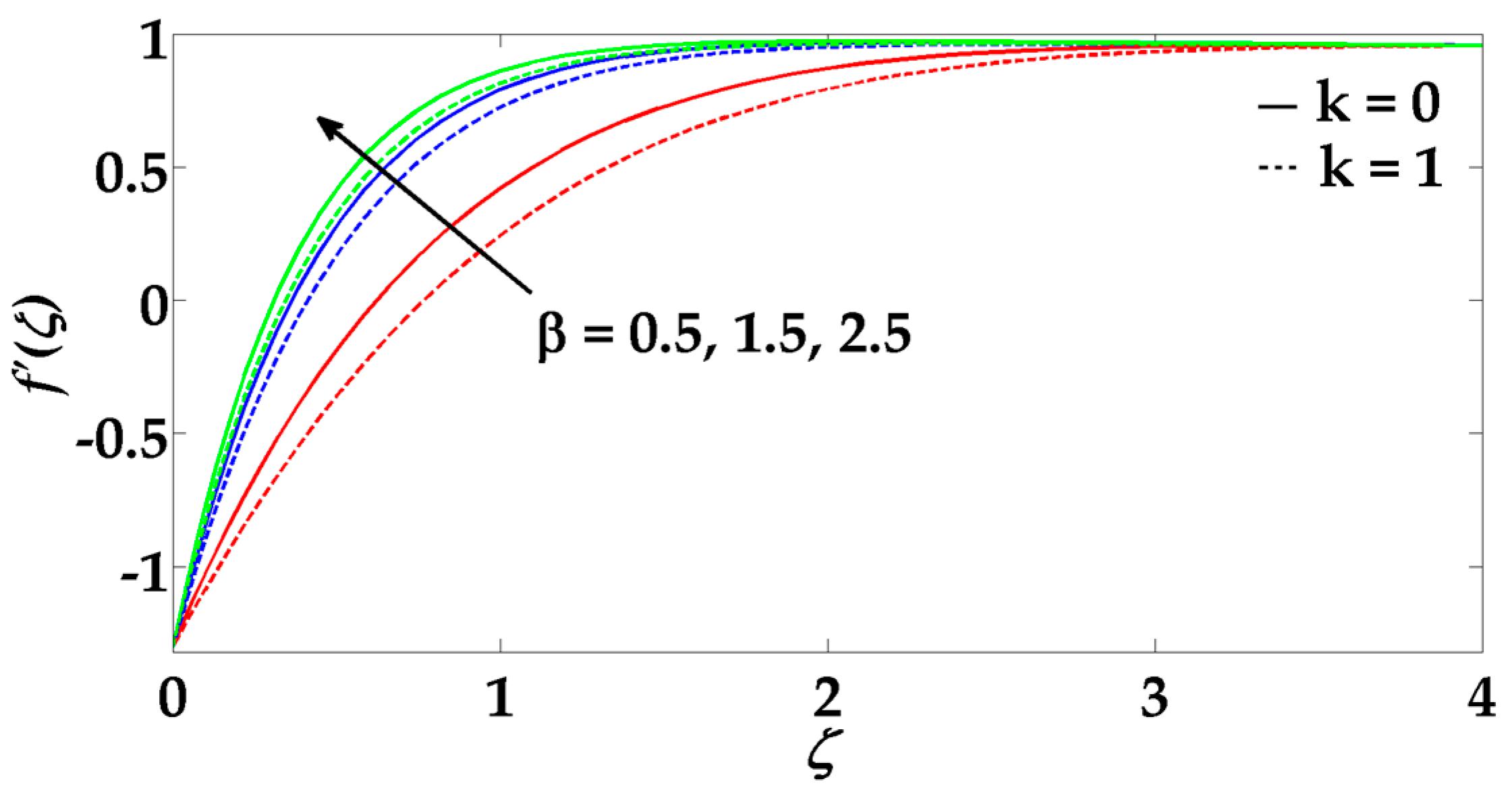
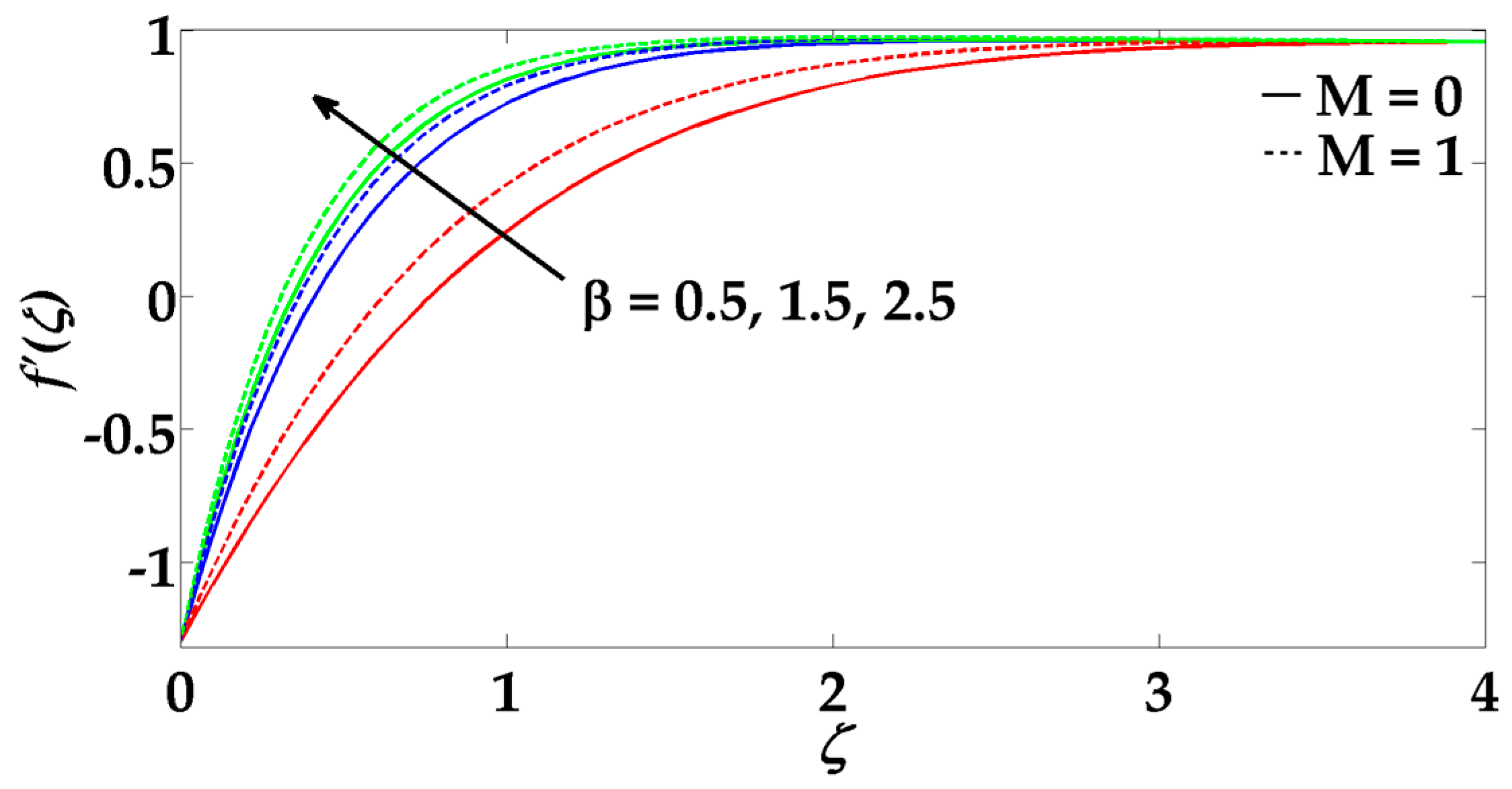
• Velocity profile decreases for magnetic parameter and porosity parameter but increases with the enhancement in Casson nanofluid parameter.
• When the Prandtl number increases, it tends to decrease the thermal boundary layer.
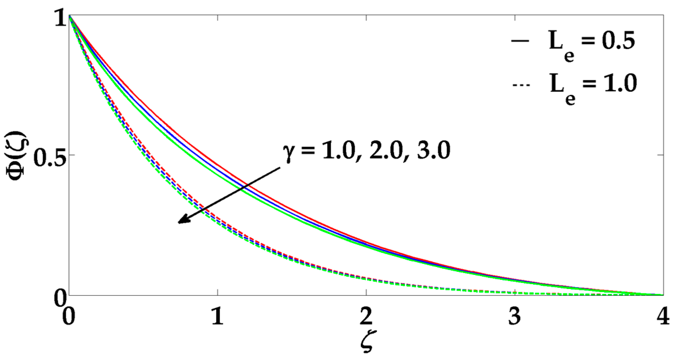
• Due to an influence of Lewis number, the concentration profile gets steeper.
• For larger values of radiation parameter, temperature profile rises.
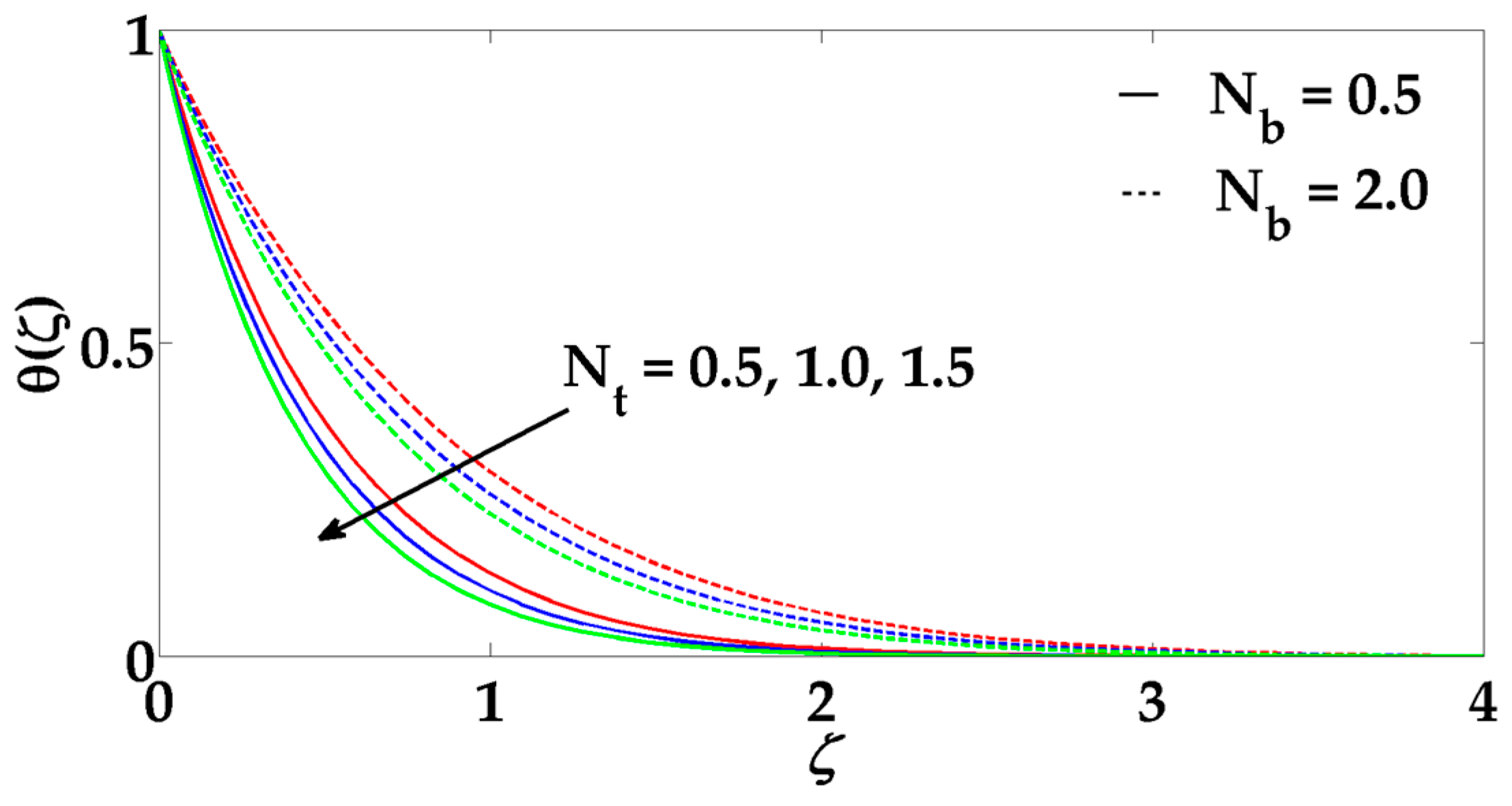
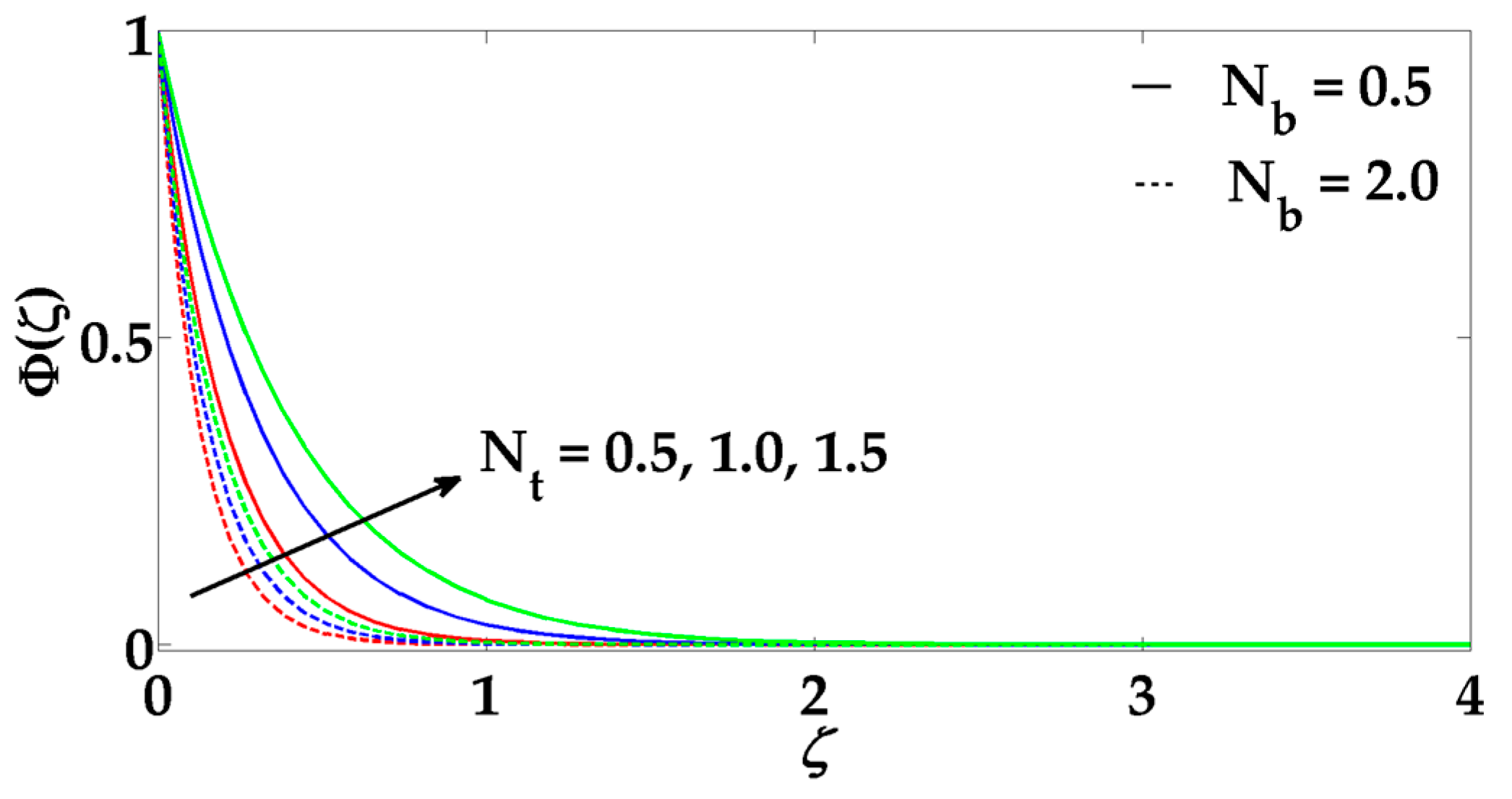
• Concentration profile decreases for higher values of$$chemical reaction parameter and Brownian motion parameter but its behaviors seem to be opposite for thermophoresis parameter increases.
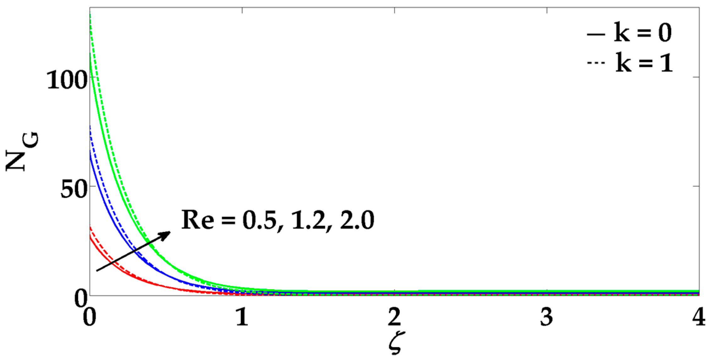
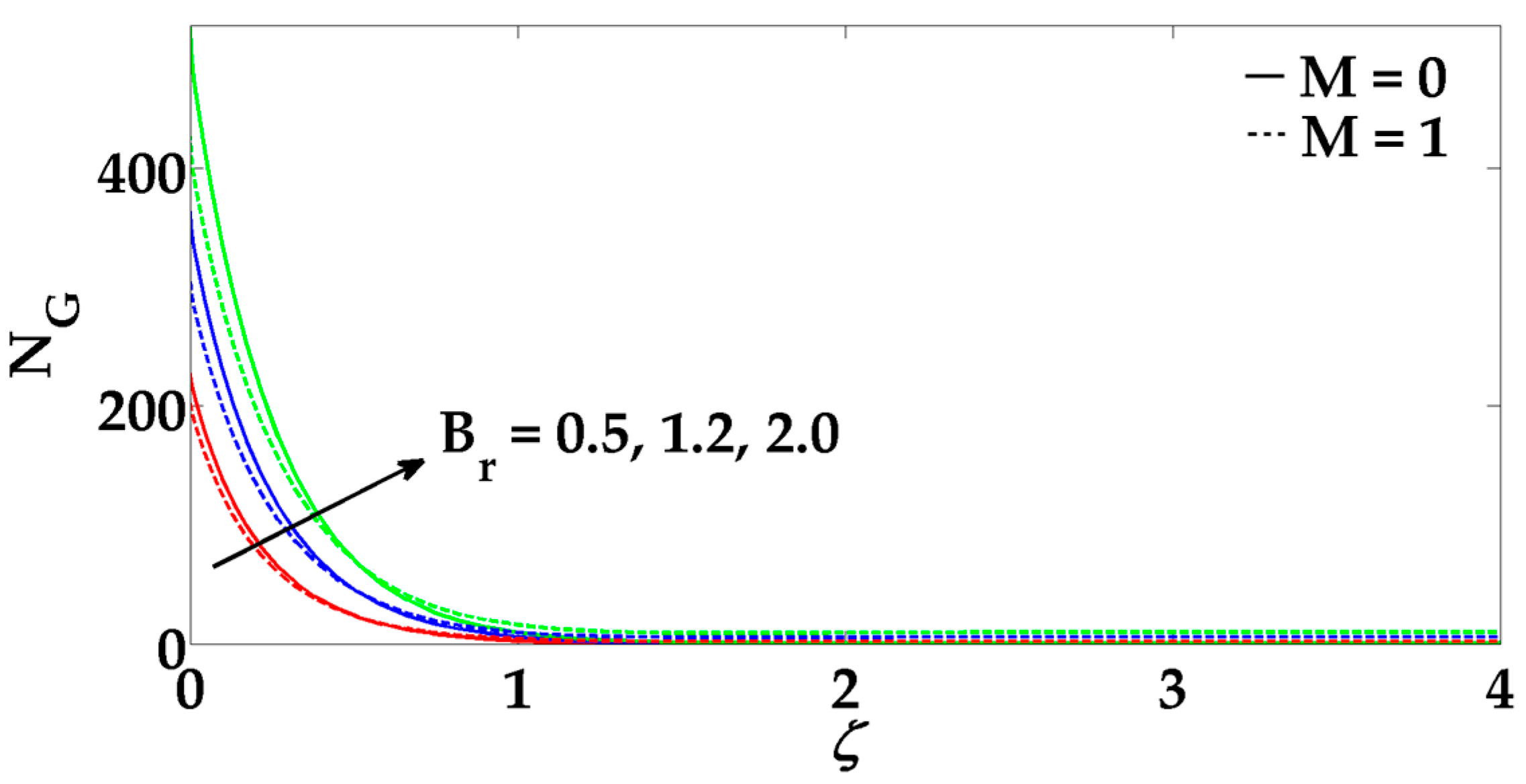
• Increasing in Brinkman number, Reynolds number, Hartmann number and porosity parameter cause an increment in the entropy generation.

References

1. Choi, S.U.S. Enhancing thermal conductivity of fluids with nanoparticles. ASME Publ. Fed. 1995, 231, 99–106. [Google Scholar]
2. Xuan, Y.; Li, Q. Investigation on convective heat transfer and flow features of nanofluids. J. Heat Transf. 2003, 125, 151–155. [Google Scholar] [CrossRef]
3. Khalili, S.; Tamim, H.; Khalili, A.; Rashidi, M.M. Unsteady convective heat and mass transfer in pseudoplastic nanofluid over a stretching wall. Adv. Powder Technol. 2015, 26, 1319–1326. [Google Scholar] [CrossRef]
4. Xiao, B.; Yang, Y.; Chen, L. Developing a novel form of thermal conductivity of nanofluids with Brownian motion effect by means of fractal geometry. Powder Technol. 2013, 239, 409–414. [Google Scholar] [CrossRef]
5. Xiao, B.; Yu, B.; Wang, Z.; Chen, L. A fractal model for heat transfer of nanofluids by convection in a pool. Phys. Lett. A 2009, 373, 4178–4181. [Google Scholar] [CrossRef]
6. Ali, M.; Zeitoun, O.; Almotairi, S. Natural convection heat transfer inside vertical circular enclosure filled with water-based Al2O3 nanofluids. Int. J. Therm. Sci. 2013, 63, 115–124. [Google Scholar] [CrossRef]
7. Ali, M.; Zeitoun, O.; Almotairi, S.; Al-Ansary, H. The effect of Alumina-water nanofluid on natural convection heat transfer inside vertical circular enclosure heated from above. Heat Transf. Eng. 2013, 34, 1289–1299. [Google Scholar] [CrossRef]
8. Zeitoun, O.; Ali, M. Nanofluid impingement jet heat transfer. Nanoscale Res. Lett. 2012, 7, 1–13. [Google Scholar] [CrossRef] [PubMed]
9. Zeitoun, O.; Ali, M.; Al-Ansary, H. The effect of particle concentration on cooling of a circular horizontal surface using nanofluid jets. Nanosc. Microsc. Therm. 2013, 17, 154–171. [Google Scholar] [CrossRef]
10. Sheikholeslami, M.; Rashidi, M.M.; Ganji, D.D. Effect of non-uniform magnetic field on forced convection heat transfer Fe3O4 water nanofluid. Comput. Method. Appl. M 2015, 294, 299–312. [Google Scholar] [CrossRef]
11. Abbas, M.A.; Bai, Y.; Rashidi, M.; Bhatti, M. Application of drug delivery in magnetohydrodynamics peristaltic blood flow of nano fluid in a nan-uniform channel. J. Mech. Med. Biol. 2015, 1650052. [Google Scholar] [CrossRef]
12. Sheikholeslami, M.; Hatami, M.; Ganji, D.D. Nanofluid flow and heat transfer in a rotating system in the presence of a magnetic field. J. Mol. Liq. 2014, 190, 112–120. [Google Scholar] [CrossRef]
13. Malvandi, A.; Hedayati, F.; Ganji, D.D. Slip effects on unsteady stagnation point flow of a nanofluid over a stretching sheet. Powder Technol. 2014, 253, 377–384. [Google Scholar] [CrossRef]
14. Abbas, Z.; Sheikh, M.; Motsa, S.S. Numerical solution of binary chemical reaction on stagnation point flow of Casson fluid over a stretching/shrinking sheet with thermal radiation. Energy 2016, 95, 12–20. [Google Scholar] [CrossRef]
15. Rashidi, M.M.; Ali, M.; Freidoonimehr, N.; Rostami, B.; Hossain, M.A. Mixed convective heat transfer for MHD viscoelastic fluid flow over a porous wedge with thermal radiation. Adv. Mech. Eng. 2014, 6, 735939. [Google Scholar] [CrossRef]
16. Nadeem, S.; Haq, R.U.; Akbar, N.S. MHD three-dimensional boundary layer flow of casson nanofluid past a linearly stretching sheet with convective boundary condition. IEEE Trans. Nanotechnol. 2014, 13, 109–115. [Google Scholar] [CrossRef]
17. Sheikholeslami, M.; Hayat, T.; Alsaedi, A. MHD free convection of Al2O3–water nanofluid considering thermal radiation: A numerical study. Int. J. Heat Mass Transf. 2016, 96, 513–524. [Google Scholar] [CrossRef]
18. Hamad, M.A.A.; Ferdows, M. Similarity solution of boundary layer stagnation-point flow towards a heated porous stretching sheet saturated with a nanofluid with heat absorption/generation and suction/blowing: A lie group analysis. Commun. Nonlinear Sci. 2012, 17, 132–140. [Google Scholar] [CrossRef]
19. Kameshwaran, P.K.; Shaw, S.; Sibanda, P.; Murthy, P.V.S.N. Homogeneous–heterogeneous reactions in a nanofluid flow due to a porous stretching sheet. Int. J. Heat Mass Trans. 2013, 57, 465–472. [Google Scholar] [CrossRef]
20. Rashidi, M.M.; Ganesh, N.V.; Hakeem, A.K.A.; Ganga, B. Buoyancy effect on MHD flow of nanofluid over a stretching sheet in the presence of thermal radiation. J. Mol. Liq. 2014, 198, 234–238. [Google Scholar] [CrossRef]
21. Sheikholeslami, M.; Ganji, D.D.; Rashidi, M.M. Ferrofluid flow and heat transfer in a semi annulus enclosure in the presence of magnetic source considering thermal radiation. J. Taiwan Inst. Chem. Eng. 2015, 47, 6–17. [Google Scholar] [CrossRef]
22. Chamkha, J. A MHD flow of a uniformly stretched vertical permeable surface in the presence of heat generation/absorption and a chemical reaction. Int. Commun. Heat Mass Trans. 2003, 30, 413–422. [Google Scholar] [CrossRef]
23. Bejan, A. Entropy Generation Minimization: The Method of Thermodynamic Optimization of Finite-Size Systems and Finite-Time Processes; CRC Press: Boca Raton, FL, USA, 1995. [Google Scholar]
24. Abolbashari, M.H.; Freidoonimehr, N.; Nazari, F.; Rashidi, M.M. Analytical modeling of entropy generation for Casson nano-fluid flow induced by a stretching surface. Adv. Powder Technol. 2015, 26, 542–552. [Google Scholar] [CrossRef]
25. Akbar, N.S.; Raza, M.; Ellahi, R. Peristaltic flow with thermal conductivity of H2O + Cu nanofluid and entropy generation. Results Phys. 2015, 5, 115–124. [Google Scholar] [CrossRef]
26. Akbar, N.S. Entropy Generation Analysis for a CNT Suspension Nanofluid in Plumb Ducts with Peristalsis. Entropy 2015, 17, 1411–1424. [Google Scholar] [CrossRef]
27. Oztop, H.F.; Al-Salem, K. A review on entropy generation in natural and mixed convection heat transfer for energy systems, Renew. Sust. Energy Rev. 2012, 16, 911–920. [Google Scholar] [CrossRef]
28. Rashidi, M.M.; Abelman, S.; Mehr, N.F. Entropy generation in steady MHD flow due to a rotating porous disk in a nanofluid. Int. J. Heat Mass Trans. 2013, 62, 515–525. [Google Scholar] [CrossRef]
29. Freidoonimehr, N.; Rahimi, A.B. Comment on effects of thermophoresis and Brownian motion on nanofluid heat transfer and entropy generation by M. Mahmoodi, Sh. Kandelousi. J. Mol. Liq. 2016, 216, 99–102. [Google Scholar] [CrossRef]
30. Bhatti, M.M.; Shahid, A.; Rashidi, M.M. Numerical simulation of fluid flow over a shrinking porous sheet by successive linearization method. Alex. Eng. J. 2016, 55, 51–56. [Google Scholar] [CrossRef]
31. Yasin, M.H.M.; Ishak, A.; Pop, I. MHD Stagnation-Point Flow and Heat Transfer with Effects of Viscous Dissipation, Joule Heating and Partial Velocity Slip. Sci. Rep. 2015, 5, 1–8. [Google Scholar] [CrossRef]
32. Aman, F.; Ishak, A.; Pop, I. Magnetohydrodynamic stagnation-point flow towards a stretching/shrinking sheet with slip effects. Int. Commun. Heat Mass Trans. 2013, 47, 68–72. [Google Scholar] [CrossRef]
33. Wang, C.Y. Stagnation flow towards a shrinking sheet. Int. J. Non-Linear. Mech. 2008, 43, 377–382. [Google Scholar] [CrossRef]
Figure 1. Geometry of the problem.
Entropy 18 00123 g001
Figure 2. Velocity profile for different values of β and k when N r = 0.5 , α = 1.3 , M = 0.1 ,   γ = 0.5 , N b = 0.5 , N t = 1.
Entropy 18 00123 g002
Figure 3. Velocity profile for different values of M and β when N r = 0.5 , α = 1.3 , M = 0.1 , γ = 0.5 , N b = 0.5 , N t = 1.
Entropy 18 00123 g003
Figure 4. Temperature profile for different values of N t and N b when N r = 0.5 ,   k = 0.1 ,   P r = 1 ,   β = 1 , α = 1.3 ,   M = 0.1 ,   γ = 0.5.
Entropy 18 00123 g004
Figure 5. Temperature profile for different values of P r and N r when k = 0.1 ,   β = 1 , α = 1.3 ,   M = 0.1 ,   γ = 0.5 ,   N t = 1.
Entropy 18 00123 g005
Figure 6. Concentration profile for different values of N t and N b when k = 0.1 , N r = 0.5 , P r = 1 ,   β = 1 , α = 1.3 , M = 0.1 ,   γ = 0.5 , L e = 3.
Entropy 18 00123 g006
Figure 7. Concentration profile for different values of f L e and γ when k = 0.1 , N r = 0.5 , P r = 1 ,   β = 1 ,   α = 1.3 , M = 0.1 , N b = 0.5 , N t = 1.
Entropy 18 00123 g007
Figure 8. Entropy profile for different values of B r and M when N r = 0.5 , P r = 1 ,   β = 1 ,   α = 1.3 ,   γ = 0.5 , N b = 0.5 , N t = 1 , L e = 3.
Entropy 18 00123 g008
Figure 9. Entropy profile for different values of Re   and k when N r = 0.5 , P r = 1 ,   β = 1 ,   α = 1.3 , M = 0.5 ,   γ = 0.5 , N b = 0.5 , N t = 1 , L e = 3.
Entropy 18 00123 g009