Article

Understanding Gating Operations in Recurrent Neural Networks through Opinion Expression Extraction

School of Computer Science and Technology, Harbin Institute of Technology, No. 92 West Da Zhi Street, Harbin 150001, China
*
Author to whom correspondence should be addressed.
Entropy 2016, 18(8), 294; https://doi.org/10.3390/e18080294
Submission received: 23 March 2016 / Revised: 18 July 2016 / Accepted: 8 August 2016 / Published: 11 August 2016

Abstract

:
Extracting opinion expressions from text is an essential task of sentiment analysis, which is usually treated as one of the word-level sequence labeling problems. In such problems, compositional models with multiplicative gating operations provide efficient ways to encode the contexts, as well as to choose critical information. Thus, in this paper, we adopt Long Short-Term Memory (LSTM) recurrent neural networks to address the task of opinion expression extraction and explore the internal mechanisms of the model. The proposed approach is evaluated on the Multi-Perspective Question Answering (MPQA) opinion corpus. The experimental results demonstrate improvement over previous approaches, including the state-of-the-art method based on simple recurrent neural networks. We also provide a novel micro perspective to analyze the run-time processes and gain new insights into the advantages of LSTM selecting the source of information with its flexible connections and multiplicative gating operations.

Graphical Abstract

1. Introduction

Extracting opinion expressions from text has been studied extensively in recent years. Various related tasks, such as opinion summarization and opinion-oriented question answering, can benefit from the extraction results. There are two types of opinionated expressions defined in the widely-used MPQA corpus [1]. Direct Subjective Expressions (DSEs) consist of explicit mentions of private opinions or emotional states, while Expressive Subjective Elements (ESEs) are words and phrases that indirectly express private attitudes. The following are some examples of the subjective expressions:
  • Zuma also [pledged]DSE continued support for Zimbabwe and its people.
  • She [congratulated]DSE him on his re-election.
  • The South African government [was happy]DSE with the SAOM report.
  • Now [all eyes are on]ESE this issue.
  • I [can never forget]DSE what I saw that day [as long as I live]ESE
  • The detainees [should]ESE be treated [as] prisoners of war according to international law.
The DSEs in the first two examples directly express private attitudes; while the DSE in the third sentence explicitly shows the emotional state. In the comparison, ESEs in the other three sentences express subjectivities in implicit ways. In Example 4, the ESE shows the writer’s high approbation for the importance of some issue without directly pointing it out. In Example 5, the DSE shows a private emotional state that the speaker was deeply impressed in a direct way, while the ESE expresses the same emotion implicitly. The word “should” in the last example shows the writer’s support of a particular issue without explicitly saying.
It is notable that the subjectivities of expressions (words or phrases) depend on not only the expressions themselves, but also the contexts. The interpretations of the same expression vary in different situations. For instance, subjectivities of the word “as” are different in Examples 5 and 6. In Example 5, the word “as” is part of ESE; while in Example 6, it appears in a phrase expressing nothing about sentiment, emotion or attitude and should be considered as non-subjective. Treating the extraction problem as a word-level sequence labeling task, it is important to involve context information in the predicting process.
A promising approach to make use of context information is learning higher-level representations of current and surrounding words automatically with deep learning technologies. Recent natural language processing (NLP) works leverage word embeddings to encode syntactic and semantic information. Composing such embeddings through a deep recurrent neural network has been proven to be an efficient way to model the interactions between words. İrsoy and Cardie conducted a comprehensive research on utilizing the Elman network, also known as a Simple Recurrent Neural Network (SRNN), in opinion expression extraction and achieved state-of-the-art performance [2].
However, the flexibilities of the compositional functions of Elman networks are limited. Simple additive compositions in Elman networks are inadequate to simulate complex language phenomenon. Research shows that multiplicative operations could accommodate more complicated interactions during representation learning [3,4]. Thus, recurrent models with multiplicative gates, such as LSTM, provide an elegant solution.
In this paper, we introduce the Long Short-Term Memory (LSTM) [5,6] recurrent neural network for opinion expression extraction. Experimentally, the proposed model outperforms previous approaches, achieving a new state-of-the-art result on the MPQA dataset.
Besides, how each part inside an LSTM block cooperates during the compositional process is rarely explored. It is difficult to improve the structures without understanding the internal coordination mechanism of such units. By analyzing the results in a micro perspective, we gain some insight into the advantages of LSTM handling opinion expressions, including (1) dividing previous memory and current input information with small recurrent connection and (2) choosing information through the element-wise multiplicative gating operations.
The major contributions of the work presented in this paper are as follows:
  • To our knowledge, this is the first work that introduces long short-term memory into the task of sentiment expression extraction.
  • We explore various structures (deep form, bidirectional form) of the network and achieve new state-of-the-art performance on the task.
  • Unlike previous works treating the networks as black boxes, we explore a new perspective to analyze the micro activations at run-time to understand the internal mechanisms.
  • Not restricted to existing researches emphasizing LSTM getting rid of the vanishing gradient problem, we firstly discuss the cooperation mechanisms of Constant Error Carousel (CEC), connection weights and multiplicative gates during information source selection through statistical experiments.
The remainder of the paper is organized as follows. In Section 2, we review some works on subjective expression extraction. Then, we introduce long short-term memory recurrent neural networks to this task in Section 3. We empirically verify the effectiveness of our method in Section 4. An insight analysis of the advantages of flexible connections and multiplicative gating operations of LSTM networks is conducted in Section 5. Finally, we conclude in Section 6.

2. Related Works

2.1. Opinion Expression Extraction

Subjective expression extraction is usually formulated as a token-level sequence labeling task with the BIO tagging scheme (“B” is for the word at the beginning of an opinion expression, “I” is for other tokens in the opinion expressions and “O” is for those outside the opinion expressions). Early works make use of context information by including features within a fixed-size window and apply linear-chain Conditional Random Fields (CRF) to predict the tag for each token [7,8]. Johansson and Moschitti provide relation information between tokens to a re-ranker by extracting features from dependency syntax and shallow semantic structures [9]. Semi-CRF based on segment-level features (such as constituents of verb phrases) also has been shown to be effective in improving the extraction performance [10].
There are also works that bring additional information during joint learning with other tasks. Choi and Cardie take attributes (polarity and intensity) of opinion expressions into consideration and improve both tasks of opinion expression identification and attribute prediction within a joint model [11]. Johansson and Moschitti extract relational features of polarity pairs from the syntactic and semantic analysis result and show that this interaction information brings obvious improvement [12,13]. Yang and Cardie formulate the opinion expression extraction and attribute classification as a segmentation problem and segment attribute classification [14]. The joint inference method with the probability-based objective function achieves a remarkable result. Besides attributes, other entities (opinion holders and targets) are also leveraged in joint models [7,15].
All above methods rely on hand-crafted features and require much engineering effort and many language-dependent resources. On the contrary, İrsoy and Cardie implement an end-to-end sequence labeler for opinion extraction with SRNN [2]. It takes unsupervised trained word vectors as input and outperforms previous approaches. However, the expressiveness of the additive function in the conventional neural unit of SRNN is limited. Compositional functions with multiplicative operations between word vectors (such as gating operations in LSTM) provide a better choice [3,4].
Liu et al. introduce LSTM networks to the task of opinion target identification [16]. Unlike most opinion targets that are noun phrases, opinion expressions vary in countless forms. Thus, identifying an subjective expression is quite a different task that requires learning complex interactions and higher level representations. Besides, unlike their work treating the network as a black box, we gain some insight into the microcosmic properties of LSTM gating operations.

2.2. Interpretability of Long Short-Term Memory

Most works treat LSTM neural networks as black boxes without discussing the sources of their advantages. Only a few works care about the internal mechanism of the LSTM memory block. For instance, there are research works that implement various variants of recurrent units with different nonlinearities, connections and gates [17,18]. They add, remove or change particular functions and gates to study the importance of these pieces in the architecture. However, these works only measure the models with the overall performance on the test set, namely the coordination mechanism of these pieces is still unknown. Not content with that, in this paper, we explore the cooperation of structures in a micro-perspective by analyzing the activations of the internal items.

3. Extraction Methodology

A Recurrent Neural Network (RNN) could get higher level representation of contexts in its hidden layer temporally [19]. It makes RNN a natural choice for the sequence labeling task.
Figure 1a shows the illustration of an RNN used as a sequence labeler to extract subjective expressions from a sentence. The RNN composes the current input of word embedding and previous hidden activation to get the higher level representation of the current time step. Such representations can be used as inputs of the softmax layer to predict the tags of the current token.
The SRNNs, such as Elman networks, compose previous hidden activations with current inputs through additive functions. However, such compositions are not powerful enough to describe the complex interactions of words, while multiplicative operations bring more flexibilities for various language phenomena [3,4]. As a kind of RNN with multiplicative gates, an LSTM could adjust inputs, outputs and stored information with the gating operations, which makes it accommodating to flexible representation composition. Moreover, the LSTM network gets access to long distance information with its memory block structure, which makes it more capable of capturing context information and learning sequence representation. The LSTM networks have been successfully applied on various tasks involving sequence data, such as phoneme classification [20], speech recognition [21], dependency parsing [21] and sentiment classification [22]. Inspired by these works, we introduce LSTM networks to the task of opinion expression extraction.
An LSTM consists of a set of self-connected subnets, known as memory blocks. Each block contains input, output and forget gates to adjust the signals inside the block. The activations of these gates G t are controlled by current input x t , previous hidden output h t 1 and the CEC state s t 1 or s t :
G I t = f U I x t + V I h t 1 + W I s t 1
G F t = f U F x t + V F h t 1 + W F s t 1
G O t = f U O x t + V O h t 1 + W O s t
where U, V and W in each formula denote the weights that connect the corresponding control signals to the gate. The subscripts I, F and O represent input, forget and output, respectively, while f is the element-wise sigmoid function. The output of the memory block h at time t is computed by:
h t = G O t s t
where ⊙ is the element-wise multiplication operator, G O t represents the output gate and s t indicates the current state of Constant Error Carousel (CEC), which is a self-connected unit:
s t = G F t s t 1 + G I t f U S x t + V S h t 1
where G I t and G F t represent the input gate and forget gate, respectively. U S and V S indicate the weight of the input connection and recurrent connection, respectively.
It is notable that s t gets access to two signals containing previous information: previous hidden output h t 1 and previous CEC state s t 1 . Thus, CEC connections provide an alternative way of capturing context information besides recurrent connections.
Figure 1b,c shows the deep form and bi-directional deep form of RNN. There are various implementations of bi-directional deep recurrent neural networks [23,24]. In this work, we leverage Schuster and Paliwal’s form [23], where the inputs of hidden layers I n p u t n get signals from both directions of other hidden layers.
I n p u t t n = W x t , if n = 1 W h t n 1 + W h t n 1 , if n > 1
where h n is the n-th hidden layer ( 1 n N ) from the input to the output. h 1 represents the first hidden layer that directly takes the embedding of current word x t as the input, while n > 1 is the identifier of the other layers. W, W and W are the corresponding weights, and arrows show the directions. Similarly, the softmax classification layer employs both forward and backward activations of the N-th hidden layer and gets context information from both directions.
y t = g U h t N + U h t N + c
where U represents the weight connecting the top hidden layer and the softmax layer and c is the bias.

4. Experiments

4.1. Dataset

The experiments are carried out on the widely-used MPQA 1.2 corpus [1]. We employ the same separation as used in [2]. Namely, we take 135 documents as the validation set and carry out the evaluation with 10-fold cross-validation on the remaining 400 documents.

4.2. Evaluation Metrics

For this dataset, it is hard to define the boundaries of opinion expressions even in manual annotation [1]. In order to get precision, recall and the F-measure, two kinds of soft metrics are used in the evaluation.
Binary overlap counts a positive true sample if there is an overlap between prediction and annotation [8]. The binary precision P b i n a r y and recall R b i n a r y can be computed as:
P b i n a r y = { p | p P c C s . t . o v e r l a p c , p } P
R b i n a r y = { c | c C p P s . t . o v e r l a p c , p } C
where C and P are the sets of correct and predicted expression spans, respectively; while || counts the number of spans in the particular set.
Proportional overlap adds up the proportions of overlaps [9]. Span coverage c v r g measures how s covers s :
c v r g s , s = s s s
where s is the length of span s. Then, span set coverage C V R G of two set of span S and S is computed as:
C V R G S , S = s j S s k S c v r g s j , s k
Finally, the proportional precision P p r o p o r t i o n a l and recall R p r o p o r t i o n a l are:
P p r o p o r t i o n a l P , C = C V R G P , C P
R p r o p o r t i o n a l P , C = C V R G C , P C

4.3. Experimental Settings

RNNLIB is a pioneer toolkit implementing the LSTM network whose code is publicly available [25]. Activations during both forward and backward propagation (even error signals propagating in each piece of the memory block) can be easily observed in this toolkit, which makes it a good choice to explore the internal mechanism of LSTM. Thus, we make use of RNNLIB to implement the recurrent architectures. Early stopping is carried out on the validation set during training. The training process stops when there is no better result after 30 epochs. We choose the publicly available word2vec embeddings learned from Google News to represent words [26]. These 300-dimensionality vectors were trained using the continuous bag-of-words architecture. The out-of-vocabulary words not contained in the Google embeddings are represented by a unified vector that initialized with random numbers on uniform distribution U 0 . 2 , 0 . 2 . We conduct no pre-training for the network, and all of the parameters (weights and biases) are initialized by sampling from a small random uniform distribution U 0 . 1 , 0 . 1 . We keep the same training parameters during stochastic gradient descent for all experiments: a learning rate of 0.005 and a momentum of 0.7.

4.4. Baseline Methods

  • Wiebe lexicon and Wilson lexicon: Breck et al. report the performances of lexicon-based unsupervised methods on this task [8]. They leverage two dictionaries of subjectivity clues (words and phrases that may be used to express private states). One is collected by Wiebe and Riloff [27], and the other one is compiled by Wilson et al. [28]. An expression is considered as a subjective one if it matches some item in the dictionary.
  • CRF: Breck et al. addressed the task with conditional random fields. Bag-of-words features, syntactic features, such as Part-of-Speech (POS) tags, and semantic features, such as the WordNet lexicon, are exploited in their work [8].
  • Semi-CRF: Yang and Cardie introduce parser results to get reliable segments for semi-Markov CRF. Segment-level features, such as syntactic categories or the polarities of words in the verb phrases, are involved to capture the context information [10].
  • +vec: İrsoy and Cardie report the performance of CRF and semi-CRF using word vectors as additional features [2]. CRF takes the word-level embeddings as features, while semi-CRF uses the mean value of word embeddings in the segment.
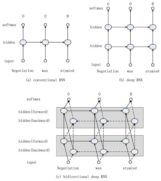
  • Bi-RNN: We take bidirectional deep Elman-type RNN as one of our baselines, which is the state-of-the-art performer on the opinion expression extraction [2].
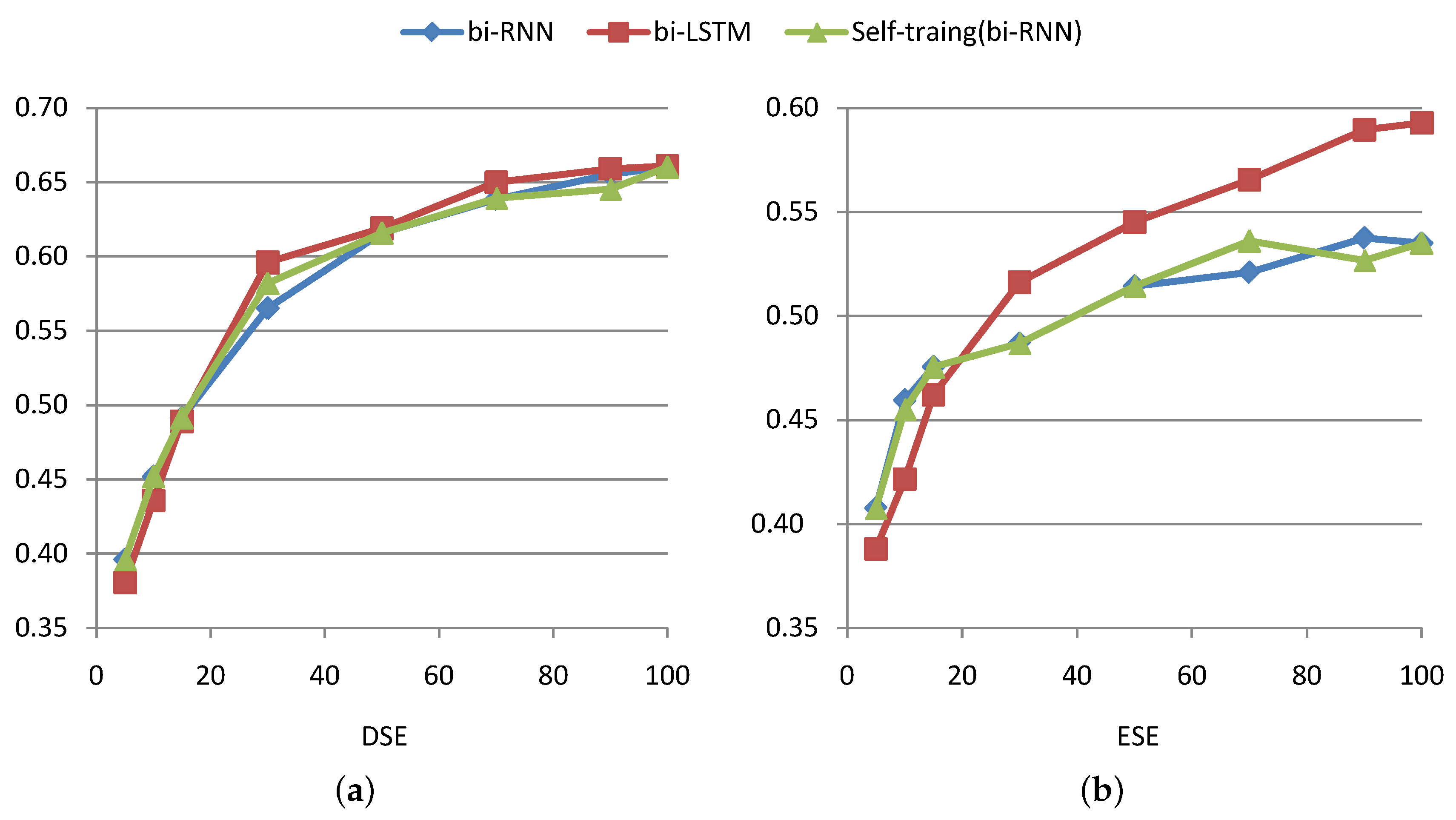
  • Self-training: We implement a self-training system based on bi-RNN, which is a strong semi-supervised baseline. The softmax layer outputs the probabilities of the three tags, and we take the highest one as the confidence level of the token. The confidence of a sentence is the mean confidences of all tokens in it. The top 200 sentences with the highest confidence are selected as additional training samples in the next iteration.
  • Joint-Loss: The joint inference approach with a probability-based objective function achieves remarkable performance [14]. To compare to their work, we test the LSTM approach in their settings.

4.5. Comparison with Feature-Engineering Methods

We conduct experiments on both DSE and ESE extractions. Table 1 and Table 2 show the comparison of the proposed method and baselines on the two kind of expressions, respectively. Numbers in bold show the highest scores. Detail settings, such as the number of hidden layers and the number of hidden units, are also provided in the tables. “Prop.” and “Bin.” represent the proportional measure and the binary measure, respectively. The performances of the supervised baseline models are reported by [2]. It is notable that, on both DSE and ESE detections, LSTMs achieve new state-of-the-art performances for both the binary overlap measure and the proportional overlap measure.
CRFs and semi-CRFs get high precisions, while recurrent models recall more positive samples and get better F-measures. Although additional word vector features encode syntactic and semantic information, CRFs with rich features still underperform recurrent models. This indicates that recurrent networks have better compositional capacities than CRFs. By composing word embeddings temporally, recurrent neural models achieve appropriate representations for context information.
For the lack of resources (such as verb phrase patterns), it is difficult to re-implement Yang and Cardie’s joint model method [14]. To compare to their work, we run the LSTM opinion expression extractor on their settings. We extract opinion expressions without distinguishing ESEs and DSEs and use the IO tagging scheme instead of the BIO scheme. Experimentally, the LSTM opinion expression extractor obtains higher F1 scores for proportional matching (65.16 vs. 64.04). We see that the LSTM compositional function could simulate the interactions of words and obtain better representation for particular tokens, even without craft context features or manually-labeled lexicons.

4.6. Comparison with Unsupervised and Semi-Supervised Approaches

It is notable that there is an obvious performance gap between lexicon-based methods and supervised models. Lexicon-based unsupervised methods are efficient and perform comparably to machine learning methods in some tasks, such as name entity recognition and aspect term extraction in a restricted domain. This is due to the fact that frequent entities in a specific domain are somehow enumerable. For example, when extracting aspect terms from laptop reviews, the physical parts of a computer can be enumerated within a lexicon. However, it is not practical to cover the diversification of various opinion expressions within a dictionary; while the higher-level representations of subjective expressions could be learned by compositional models, such as RNNs.
The self-training system is compared to recurrent-based models on different fractions of data. The results are shown in Figure 2.
According to the experimental results, the performance of bi-RNN is quite similar to that of the self-training baseline based on bi-RNN. Even on the small fraction of data, the difference is not significant. This is due to the fact that it is difficult to get the correct tags with high confidence when the data are sparse, especially in the task of sequence labeling with imbalanced class distribution. Despite performing similar as the baselines in the DSE dataset, LSTM learns more appropriate representations and outperforms both bi-RNN and the self-training system on ESE extraction when the data are more than 30%.

4.7. Comparison with the Elman Network

LSTM outperforms SRNN on ESE extraction by 2.4% for the proportional overlap measure and by 4.0% for the binary overlap measure; while on DSE extraction, there is no palpable improvement. This is due to the fact that ESEs are a more flexible linguistic phenomenon, which LSTM could accommodate better. The subjectivity in an ESE is expressed in an implicit way. The lengths of ESE varies and most words in them are neutral. The sentiment information of these phrases is carried out by the interactions of context words rather than the words themselves. Simple additive compositional functions relying on the recurrent connections in SRNNs are limited in simulating complex interactions, while element-wise multiplicative operations in LSTMs provide more flexibilities. The internal reason for such a phenomenon will be further discussed in Section 5.

4.8. Network Parameters

The performances of LSTMs with different hyperparameter settings are shown in Figure 3. We conduct experiments on various depths (numbers of hidden layers), hidden sizes (numbers of units in each hidden layer) and directionality.
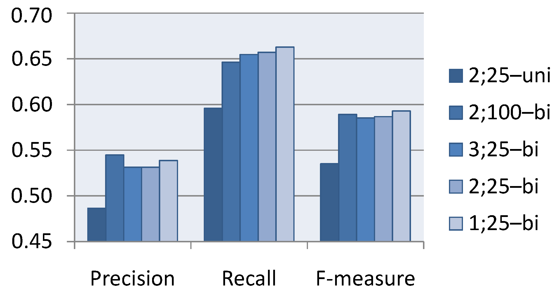
  • Hidden size : Experimentally, LSTM networks with 25 blocks in the hidden layer, producing better results (about by 1%) compared to those with 100 hidden blocks; while the situation is opposite in the Elman network. This suggests that LSTM blocks with multiplicative gates provide more flexible compositional functions, even with a smaller hidden size.
  • Depth of networks: Networks with 1–3 hidden layers produce a similar precision, recall and F-value. Different depths lead to variation by less than 0.7%, and the one hidden layer shallow form performs best. This indicates that the LSTM units have the capacity to simulate a complex composition that SRNN could only accommodate with deep cascaded nonlinearities.
  • Directionality: Bidirectional networks outperform unidirectional networks by 6.2% on DSE and by 5.2% on ESE. We see that bidirectional LSTMs get access to the future words and provide more context information.

5. Interpretable Analysis

Most works treat LSTM neural networks as black boxes, and only a few works discussed the internal cooperation mechanism of the items in an LSTM memory block. In this section, we explore the cooperation of structures in a new micro-perspective by analyzing internal activations.
Now that we discover that the long short-term memory network achieves a better performance than simple RNN on ESE extraction, we will explore: (1) in which cases LSTM works better; (2) what kinds of properties lead to these cases; and (3) how the LSTM structure achieves such properties. All of the explorations are conducted on the dataset of ESE.
More specifically, we find three patterns where LSTM outperforms SRNN significantly in Section 5.1. In Section 5.2, we focus on one of the patterns (“as” phrases) and show that LSTM achieves better context adaptability than SRNN. To further explain the results, in Section 5.3, we show that LSTMs have the capacity to select current or context information independently, which is an advantage over SRNN rarely observed or mentioned in previous works. In Section 5.4, by analyzing the activations at expression boundaries, we show that the adaptive ability of forget gates makes LSTM more flexible and expressive than SRNN. We conclude this in Section 5.5.

5.1. Finding Improved Patterns

5.1.1. Motivation for Finding Improved Cases

Since the result in Section 4.5 shows that LSTM outperforms SRNN, we would like to find some cases in which LSTM handles significantly better than SRNN. For example, we explore whether LSTM predicts the tags more accurately than SRNN when the current word is a noun or the current word is the first word of the sentence. Such cases provide intuitions about the difference between the two models. Additionally, we can take these cases or patterns as clues to further explore the internal mechanism of the advantages of LSTM.

5.1.2. Significance Test on the Difference of Single-Word Pattern Predicting

To analyze the advantages of LSTM, we conduct experiments to discover for which kinds of expressions LSTM improves the recognition rate notably. It is hard to design a taxonomy for various multi-word opinion expressions. Hence, here, we only focus on the single-word level, explicitly on what kinds of words LSTM works better for compared to SRNN according to the two-sided paired t-test on the 10-fold cross-validation. Various hypotheses based on Part-of-Speech (POS) tags, positions of words and specific words are tested.
Table 3 shows the candidate patterns for which we conduct the significance test. The POS tags are labeled using the Stanford POS tagger (http://nlp.stanford.edu/software/tagger.shtml). There are 45 different tags in the Penn Treebank English POS tag-set (http://www.comp.leeds.ac.uk/amalgam/tagsets/upenn.html). We merge nine different punctuation tags into one single tag that indicates that the current token is a punctuation without distinguishing detailed functions. The same integrations are conducted on nouns, adjectives, adverbs and verbs. After merging the tags in the same categories, 25 different POS tags are considered as patterns of words. Besides the POS categories and two positions, we also explore whether LSTM performs better when tagging specific words. To ensure that the sample set is big enough, we only select words appearing more than one thousand times in the corpus. Finally, there are 35 frequently-used words selected as candidate patterns to be tested.
The experimental result is shown in Table 4. There are three cases where LSTM outperforms simple RNN significantly (according to the two-sided paired t-test with a confidence level of α = 0 . 05 ). We see that LSTM predicts the tag more accurately than SRNN when: (1) the current input is adverb; (2) the current input is the first word of the sentence; or (3) the current input is the word “as”.
Although adverbs and the first words of the sentences are better classified by LSTM, the usage of these word is complex. It is complicated to summarize specific functions or application scenarios for them. In the following subsections, we focus on the word “as” and related phrases to explore the properties and internal cooperation of LSTM.

5.2. Comparison of the Context Adaptability of Recurrent Models

In this subsection, we focus on the tags of the word “as” in different phrases, which belong to one of the patterns extracted in Section 5.1, and show that LSTM accommodates better the interactions of contexts than SRNN in such phrases.

5.2.1. Context Dependence of Tags of the Word “as”

In the real-world data, there are some words expressing nothing about sentiment or private state on its own. Whether such a word is considered as a part of opinion expression is decided by the context. The word “as” is a typical case where the tag depends on the context indicators.
For instance, phrases like “as adjective/adverb” are usually used to express comparison or expectations, while “as noun” phrases are used to enumerate mentioned things. Hence, whether the word “as” is in an opinion expression is greatly influenced by following word in real-world data.
Besides that, in phrases “as adjective/adverb as” or “as long as”, the word “as” is likely to be a token in an expressive subjective expression. Such “as ... as” patterns get a greater possibility to be opinion expressions than single “as” (35.5% (most non-sentiment ones are conjunction phrases like “as well as” and preposition phrases like “as far as”) vs. 13.8% in ESE annotation in MPQA). By contrast, in phrase like “as ... said”, the word “as” tends to be a non-sentiment preposition outside the subjective expressions. Only 10% of the “as” in such phrases are the expressive subjective MPQA corpus. The statistical result is consistent with people’s intuition and common sense.

5.2.2. Experiment about Context Adaptability

As describe in Section 5.2.1, the tag of the word “as” is decided by the context. It is useful to know whether LSTM and SRNN could learn such a trait. More explicitly, taking the First word “As” (FA) in phrases as objects of observation, we consider a model having high context adaptability if it could learn the following interactions:
  • Contiguous interaction: the tag of FA is influenced by the later word. For instance, FA followed by an adjective or adverb (e.g., as quickly) tends to be part of opinion expression, while FA followed by a noun (e.g., as China) is not. We would like to explore whether LSTM and SRNN are sensitive to this difference.
  • Divorced interaction: the tag of FA is influenced by words that are not directly adjoined. For instance, in the phrases “as ... as” and “as ... said”, the labels of FAs should be predicted differently. We will show how LSTM and SRNN could accommodate the different situations.
If the prediction results of the tags of FAs of a model manifest the above two interactions, we learn that such a model gains context adaptability. To explore such a property in LSTM and SRNN, we train the two models on the MPQA ESE corpus with the same experimental settings as described in Section 4 and observe how the predictions of the labels of FAs change with respect to different contexts. To get test sets of different forms of “as” phrases, we extract non-sentiment nouns and sentiment modifiers to generate different expressions. We extract 800 Adjectives/Adverbs (ADs) most frequently used in the MPQA corpus and contained in a widely-used sentiment lexicon [29]. Correspondingly, 800 highest frequency Nouns (NNs) not existing in the sentiment lexicon are selected. With these extracted words, the test set of six experimental groups with different phrase forms is built (as shown in Table 5). Groups named with A or N indicate that they contain Adjectives/Adverbs (ADs) or Nouns (NNs) respectively. While symbols +, − or # show that the phrase forms are “as ... as”, “as ... said” or “as” followed by a single word, respectively. Each group contains 800 phrases that begin with the word “as”.
According to the standards of annotation, the “as ... as” phrases with sentiment modifiers in the middle (e.g., “as friendly as”) actually express subjective attitudes (conjunction phrases like “as well as” and preposition phrases like “as far as” are widely used in the real-world corpus and express no subjective attitudes. However, they are not included in the generated phrases), while FAs in phrases like “as ... said” with nouns in the middle (e.g., “as he said”) are non-sentiment prepositions. Thus, FAs of phrases in Group +A could be generally labeled as the beginnings of opinion expressions (“B”), while those in the −N group are tagged as “O” (words outside ESEs). Conservatively, we cannot affirm the standard labels for other groups, because it is hard to decide the subjectivities. The subjectivities of phrases in the # groups are controversial, while phrases in the +N and −A groups rarely exist in the real-world data.
To show in detail how context words influence FAs, we compute the proportions of FAs tagged as “B” (beginning of an opinion expression) in these groups, which are the indicators of the context sensitivities of the two models. If the proportions change obviously with respect to different context groups, we learn that the model could gain high context adaptability. Knowing the standard tags in the +A and −N groups, we can also get the accuracies of the two models predicting the tags of FAs in these two groups. These accuracies provide the intuition about why LSTM outperforms SRNN when handling “as” phrases.
Table 5 shows the experimental results. The third and fourth columns show the proportions of FAs tagged as “B” in different models, while the fifth and sixth columns present the accuracies.
Most notably, LSTM is more sensitive to the context words than SRNN. According to the result, for LSTM, about half of the FAs are tag as “B” in the A groups, and only less than 6% of those are labeled as “B” in the N groups; while SRNN produces similar results for the A groups and the N groups. Although the accuracies of the two models on the −N group are similar, prediction performance on the +A group shows a significant difference. We see that LSTM adapts to the context information better, while SRNN does not change much regardless of the context.
Furthermore, By comparing the +, # and − groups, it can be inferred that the non-adjacent context words also bring bias through the LSTM network. The difference between groups is consistent with real-world training data, which indicates that the LSTM structure has the capacity to learn such patterns and interactions for both contiguous context and divided context.

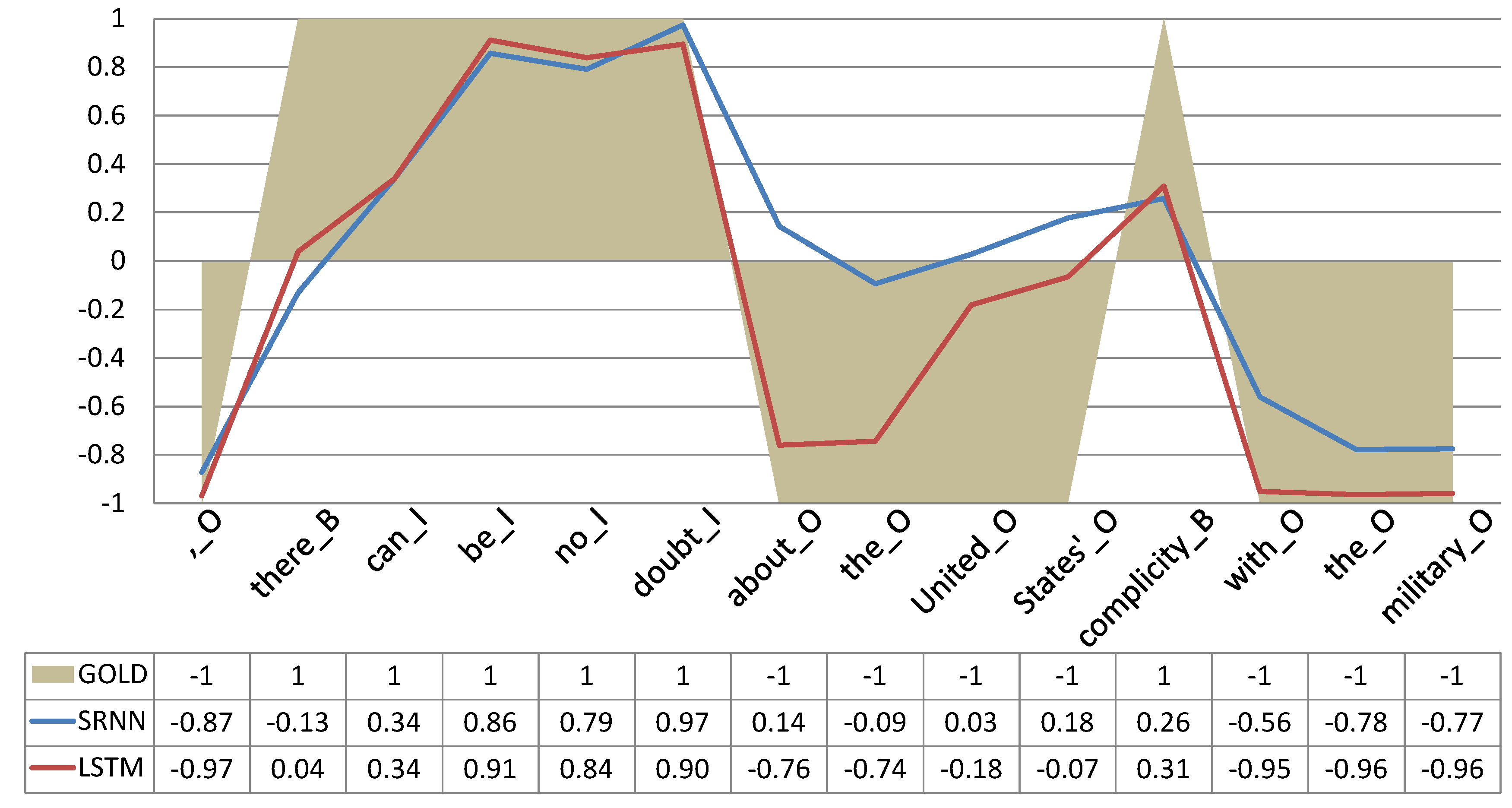
5.2.3. Visualization of the Internal Activations of LSTM

To visualize the internal activations of LSTM, we randomly select five NNs and five ADs and get the hidden outputs of FAs in the corresponding phrases in the six groups. An alternative least-squares scaling is implemented based on the Euclidean distance between output activations.
Figure 4 shows the distances of these outputs in a two-dimensional illustration. Phrases that tend to be opinion expressions (A groups and + groups) distribute in the upper right part; while the bottom left contains the phrases more likely to be objective (N groups and − groups). It is obvious that both AD and “as” at the end of the phrase bring positive (word belonging to an opinion expression) information through the temporal processing of LSTM, while NN and “said” bring negative information. Namely, both contiguous interaction and divorced interaction influence particular tokens through the LSTM network.

5.3. Internal Analysis: Gating Selection of Information

We have shown that there is a gap of context adaptability between LSTM and SRNN in Section 5.2. In this subsection, we explore the source of the difference and discuss the capacity of LSTM dividing current and context signals, providing a new perspective of the advantages of LSTM.

5.3.1. Motivation of the Analyzing Internal Mechanism of LSTM

As shown in Section 5.2, LSTM shows context sensitivities when handling “as” phrases, while SRNN does not. This indicates that, between the two models, there is a capacity gap of learning higher-level representations for a particular time step. It would be useful to know the internal mechanisms difference between the LSTM memory block and the SRNN unit that lead to such a gap.
Most existing works treat LSTM as a black box without studying how the memory blocks achieve more flexible compositional functions than SRNN units. Not content with that, we explore the determinant of context sensitivity and discuss the cooperation mechanism between internal pieces of the structure.

5.3.2. Finding Determinant of Context Sensitivity

There are many factors (gates and weights) influencing the final outputs of the memory blocks and leading to the difference of tags between A groups and N groups. In this part, we trace back to the source of the difference step by step.
We conduct our study on the structure with only one hidden layer, which is the best performer in the experiment. According to Formula (7) in Section 3, the labels of the tokens are decided by both forward (left-to-right) and backward (right-to-left) units. However, the left-to-right signals only contain the input activations of FAs, which are the same (all of them are word embeddings of the word “as”) in all groups and bring no difference to the representations. Thus, we only focus on the internal activations of right-to-left connections. We use h t to represent h t in the following part for convenience; other symbols are simplified in the same way.
As shown in Figure 4, the outputs h t of the A and N groups are distinguished. To explicitly evaluate the degree of separation, we consider the activation vectors as the points in the high-dimensional space and use a Ratio of Overlap ( R O ) measure to evaluate the proportion of two groups of points mixed together. If the R O value is high, this indicates that the activations are not well distinguished; and if the R O is a small value, we learn that the points in the high-dimensional space are almost linear separable in the softmax layer.
Furthermore, by analyzing the R O values of the factors in the forward propagation process, we can figure out the source of difference in the A and N groups. Then, such source factors can be considered as the determinants of the context sensitivity of LSTM. For instance, according to Formula (4), h t is decided by G O t and s t . Experimentally, G O t of the A and N groups are mixed together, while s t of the two groups are distinguished. Thus, we can identify that s t is the determinant of the difference in this compositional process. By analyzing the determinants step by step, we can gain insight into the internal mechanism of the LSTM compositional process.
The R O value can be computed as:
R O = i = 1 S o v e r l a p v i , c A , c N S
where S represents the sample set and S is the number of samples; half of the points in S are randomly selected from the A group, and the other half are from the N group. v i indicates the i-th activation vector in S, while C A and C N represent the geometrical center of the A group and the N group respectively. We count an overlap if the activation is closer to the center of the opposite group than that of the group to which it belongs.
o v e r l a p v i , c A , c N = 1 , if d v i , c A , c N > 0 0 , otherwise
d v i , c A , c N = d i s t a n c e v i , c A d i s t a n c e v i , c N , if v i A d i s t a n c e v i , c N d i s t a n c e v i , c A , if v i N
where d i s t a n c e indicates the Euclidean distance between two vectors.
The R O value is less than 0.5 if there is no outlier. Experimentally, the R O value of two groups of randomly-generated points is about 0.488. In order to find the source of the difference of activations, we calculate the R O values of several intermediate results during the forward propagation process in LSTM. One-thousands samples are randomly selected (500 in the −A group and 500 in the −N group). The results are shown in Table 6.
It is easy to find that the output gate activations G O t are similar in A groups and N groups. Thus, according to Formula (4), the main difference between the A and N groups is generated in CEC unit activations s t . The two factors influencing s t in Formula (5) are also observed with the R O measure. Signals through input gate G I t f U S x t + V S h t 1 in A groups and N groups are similar, while previous information through forget gate G F t s t 1 is the main determinate of the difference.

5.3.3. Independence of Current and Previous Signals in LSTM

As shown in Section 5.3.2, although the previous information is contained in h t 1 , the signals getting through input gates G I t f U S x t + V S h t 1 show rare differences between the A and N groups. We analyze the connection weight V S and U S to explore the importance of each factor. The histograms of the statistical distribution of the absolute values of the two weights are shown in Figure 5.
It is notable that V S is much smaller than U S ; the average absolute value of V S is only one-eighth of that of U S . With the connection weights close to zero, the signals of V S h t 1 become negligible. Namely, the state in CEC unit s t can be describe as:
s t G F t s t 1 + G I t f U S x t
It can be inferred that the information of the context almost comes from the CEC connection G F t s t 1 , while the input signal of the current word is adjusted through input gate G I t f U S x t . In this way, the LSTM network divides the current input signal and previous memory of the context and makes it possible to select different information sources via gates based on different current or context information; while SRNN is limited to fixed weights and gains less flexibility.
The negligible weight of V S is constant after training and influences all test cases not restricted to the “as” phrases. Thus, during the test process, all cases can benefit from the independence of current and previous information since LSTM could select information from the two source independently via the gates for all inputs.
As a matter of fact, we provide two examples of the advantages of such independence in this paper. For the cases of “as” phrases, we show how the LSTM model adapts to the previous signal and blocks the input in Section 5.3.4. Meanwhile, to further demonstrate the flexibility of LSTM, we provide situations where LSTM forgets the context and lays stress on the current input in Section 5.4.
There are other patterns extracted in Section 5.1 where LSTM outperforms SRNN. The application situations of these cases, such as adverbs, are complicated and not suitable to be analyzed as instances here. However, since same connection weights are shared in all test cases, the process handling these patterns is also covered by the generality of Formula (17).

5.3.4. Information Selection in “as” Phrases

Since we know that an LSTM has the capacity to adjust the current and previous signal independently, we can describe the difference of the process of LSTM and SRNN handling “as” phrases. Figure 6 shows the illustration of the internal mechanisms of SRNN and LSTM units at the run-time of the test. It is notable that each gate G t (no matter whether an input gate or a forget gate) is represented by a vector of real numbers g h t 0 , 1 , and the length of the vector is equal to the size of hidden layer H.
G t = g 1 t , g 2 t , . . . , g H 1 t , g H t
If most numbers in the gate vector are close to zero, the signal getting through it will be squashed to a very small value after element-wise multiplicative operation. Thus, we consider that the gate blocks the signal if most numbers in the gate vector are close to zero instead of one, and the mean value m t of these numbers is the appropriate metric indicating the gate blocking or keeping the information.
m t = 1 H g h t H
Specifically, for the convenience of understanding, if the mean value m t of the real numbers in a gate vector (which may be the input gate or forget gate here in Figure 6) is less than 0.3 (which is an empirical threshold small enough to ensure the signal through the gate becoming less crucial), we consider that the gate blocks most information and tag it as a “close” gate in Figure 6. SRNN shares same connection weight every time step, getting information from both connections no matter what the current input is; while LSTM could select the sources of information through the gating operation according to different current input and context information. As shown in Figure 6a,b, in the right-to-left precess, SRNN gets information from both the previous adjective and current “as”, while LSTM squashes the input to a very small value (with the average input gate value less than 0.3) and gets major sentiment information from the previous state in the CEC unit. This leads to the large flexibility gap of the two models accommodating the context information as described in Section 5.2: SRNN tags most beginning words as non-sentiment, while LSTM could adapt to the following words.
Meanwhile, in (backwardly) the previous time step, as visualized in Figure 6c,d, LSTM gets information from both sources with both gates open, bringing information of the continuous word, as well as the disconnected token to the leftmost tag.

5.4. Forget at the Boundary

During the cross-validation, it is also found that, at the edges of the opinion expressions, the outputs of LSTM change more dramatically and sensitively than SRNN. Before statistical analysis, we firstly show an example to visualize such a phenomenon. We use d to describe the algebra difference of the probability of the current word being in or not in an opinion expression.
d t = m a x p ( y t = B ) , p ( y t = I ) p ( y t = O )
where p is computed based on the softmax activations. Thus, d 1 , 1 represents the confidence of models tagging the specific word as part of the sentiment expression. If d t > 0 , the t-th token tends to be part of the opinion expression and will be tagged as “B” or “I”, while d t < 0 indicates that the word is outside subjective expressions and will be tagged as “O”.
The d values of all input time steps in the example are plotted in Figure 7. It could be found that the LSTM curve adapts quickly to the gold standard (“GOLD” area in the figure) binary-value of −1 and one, while the SRNN curve changes slowly and misclassifies several tokens.
Generally, the LSTM curve is steep, while the SRNN curve is gentle. To explicitly evaluate it, we compute the output change ( O C ) of the confidence in one time step:
O C = d t d t 1
and compare the output change on the edges of opinion expression between LSTM and SRNN.
Table 7 shows the comparison of the output change at the boundaries of opinion expressions. LSTM shows a more dramatic approximation to the annotated label than SRNN.
As described in Section 5.3, the information of the previous time step almost comes from the CEC unit through the forget gate. Statistically, the average value of the activations of forget gates at boundaries is smaller than that not at the edges (0.483 vs. 0.549), namely LSTM actually tends to forget the context at the boundaries of opinion expressions. In this way, the output could change more dramatically and lead to a steep curve simulating the gold standard value better. Such an adaptive ability of forget gates makes the model more flexible and expressive than SRNN.

5.5. Source of the Advantages of LSTM

We have described how LSTM adapts to the context information in Section 5.3 and how the network forgets the context in Section 5.4. Through these two instances, we can gain an insight into the advantages of LSTM over SRNN.
SRNN shares same eclectic connection weight every time step, while LSTMs: (1) provide alternative access to context information besides recurrent connection through CEC units; (2) could divide the source of current and context signals with (almost) blocked recurrent connection by learning a negligible weight; (3) select the sources of information through multiplicative gating operations according to different current input and context information; and (4) finally, achieve a more flexible and suitable representation.

6. Conclusions

In this paper, we have explored extracting opinion expressions with long short-term memory. Tested on a public dataset, the proposed architecture achieves new state-of-the-art results, outperforming CRF-based models and deep Elman-type RNNs on both ESE and DSE extractions. Bidirectional LSTMs gain remarkable capacities to learn context interactions even in a shallow form with a relatively small hidden size. Not content with leaving the internal mechanism of LSTM unknown, we also analyze internal activations of LSTM in a new micro perspective. We gain some insight into the advantages of LSTMs handling opinion expressions, including dividing previous memory and current input with small recurrent connection and choosing information through the element-wise multiplicative gating operations.

Acknowledgments

This work is supported by the projects of the China Postdoctoral Science Special Foundation (No. 2014T70340), the National Natural Science Foundation of China (No. 61300114 and No. 61572151) and the Specialized Research Fund for the Doctoral Program of Higher Education (No. 20132302120047).

Author Contributions

Xin Wang, Yuanchao Liu and Xiaolong Wang put forward the original ideas of this research after many discussions. Xin Wang and Yuanchao Liu performed the experiments and wrote and revised the main part of the paper. Chengjie Sun, Ming Liu and Xiaolong Wang contributed materials, reviewed and modified the paper. All authors have read and approved the final manuscript.

Conflicts of Interest

The authors declare no conflict of interest.

References

  1. Wiebe, J.; Wilson, T.; Cardie, C. Annotating expressions of opinions and emotions in language. Lang. Resour. Eval. 2005, 39, 165–210. [Google Scholar] [CrossRef]
  2. İrsoy, O.; Cardie, C. Opinion mining with deep recurrent neural networks. In Proceedings of the 2014 Conference on Empirical Methods in Natural Language Processing, Doha, Qatar, 25–29 October 2014; pp. 720–728.
  3. Socher, R.; Perelygin, A.; Wu, J.Y.; Chuang, J.; Manning, C.D.; Ng, A.Y.; Potts, C. Recursive deep models for semantic compositionality over a sentiment treebank. In Proceedings of the Conference on Empirical Methods in Natural Language Processing, Seattle, WA, USA, 18–21 October 2013; pp. 1631–1642.
  4. İrsoy, O.; Cardie, C. Modeling compositionality with multiplicative recurrent neural networks. In Proceedings of the International Conference on Learning Representations (ICLR), San Diego, CA, USA, 7–9 May 2015.
  5. Hochreiter, S.; Schmidhuber, J. Long short-term memory. Neural Comput. 1997, 9, 1735–1780. [Google Scholar] [CrossRef] [PubMed]
  6. Gers, F. Long Short-Term Memory in Recurrent Neural Networks. Ph.D. Thesis, Universität Hannover, Hannover, Germany, 2001. [Google Scholar]
  7. Choi, Y.; Breck, E.; Cardie, C. Joint extraction of entities and relations for opinion recognition. In Proceedings of the 2006 Conference on Empirical Methods in Natural Language Processing, Sydeny, Australia, 22–23 July 2006; pp. 431–439.
  8. Breck, E.; Choi, Y.; Cardie, C. Identifying expressions of opinion in context. IJCAI 2007, 7, 2683–2688. [Google Scholar]
  9. Johansson, R.; Moschitti, A. Syntactic and semantic structure for opinion expression detection. In Proceedings of the Fourteenth Conference on Computational Natural Language Learning, Uppsala, Sweden, 15–16 July 2010; pp. 67–76.
  10. Yang, B.; Cardie, C. Extracting opinion expressions with semi-markov conditional random fields. In Proceedings of the 2012 Joint Conference on Empirical Methods in Natural Language Processing and Computational Natural Language Learning, Jeju Island, Korea, 12–14 July 2012; pp. 1335–1345.
  11. Choi, Y.; Cardie, C. Hierarchical sequential learning for extracting opinions and their attributes. In Proceedings of Annual Meeting of the Association for Computational Linguistics, Uppsala, Sweden, 11–16 July 2010; pp. 269–274.
  12. Johansson, R.; Moschitti, A. Extracting opinion expressions and their polarities—Exploration of pipelines and joint models. In Proceedings of the 49th Annual Meeting of the Association for Computational Linguistics: Human Language Technologies, Portland, OR, USA, 19–24 June 2011; Volume 2, pp. 101–106.
  13. Johansson, R.; Moschitti, A. Relational features in fine-grained opinion analysis. Comput. Linguist. 2013, 39, 473–509. [Google Scholar] [CrossRef]
  14. Yang, B.; Cardie, C. Joint modeling of opinion expression extraction and attribute classification. Trans. Assoc. Comput. Linguist. 2014, 2, 505–516. [Google Scholar]
  15. Yang, B.; Cardie, C. Joint Inference for Fine-grained Opinion Extraction. In Proceedings of the 51st Annual Meeting of the Association for Computational Linguistics, Sofia, Bulgaria, 4–9 August 2013; pp. 1640–1649.
  16. Liu, P.; Joty, S.; Meng, H. Fine-grained opinion mining with recurrent neural networks and word embeddings. In Proceedings of the Conference on Empirical Methods in Natural Language Processing, Lisbon, Portugal, 17–21 September 2015.
  17. Jozefowicz, R.; Zaremba, W.; Sutskever, I. An empirical exploration of recurrent network architectures. In Proceedings of the 32nd International Conference on Machine Learning, Lille, France, 6–11 July 2015; pp. 2342–2350.
  18. Greff, K.; Srivastava, R.K.; Koutník, J.; Steunebrink, B.R.; Schmidhuber, J. LSTM: A Search Space Odyssey. 2015; arXiv:1503.04069. [Google Scholar]
  19. Elman, J.L. Finding structure in time. Cognit. Sci. 1990, 14, 179–211. [Google Scholar] [CrossRef]
  20. Graves, A.; Schmidhuber, J. Framewise phoneme classification with bidirectional LSTM and other neural network architectures. Neural Netw. 2005, 18, 602–610. [Google Scholar] [CrossRef] [PubMed]
  21. Graves, A.; Mohamed, A.R.; Hinton, G. Speech recognition with deep recurrent neural networks. In Proceedings of the 2013 IEEE International Conference on Acoustics, Speech and Signal Processing, Vancouver, BC, Canada, 26–31 May 2013; pp. 6645–6649.
  22. Tai, K.S.; Socher, R.; Manning, C.D. Improved semantic representations from tree-structured long short-term memory networks. In Proceedings of the 53rd Annual Meeting of the Association for Computational Linguistics and the 7th International Joint Conference on Natural Language Processing of the Asian Federation of Natural Language Processing, Beijing, China, 26–31 July 2015; pp. 1556–1566.
  23. Schuster, M.; Paliwal, K.K. Bidirectional recurrent neural networks. IEEE Trans. Signal Process. 1997, 45, 2673–2681. [Google Scholar] [CrossRef]
  24. Baldi, P.; Brunak, S.; Frasconi, P.; Soda, G.; Pollastri, G. Exploiting the past and the future in protein secondary structure prediction. Bioinformatics 1999, 15, 937–946. [Google Scholar] [CrossRef] [PubMed]
  25. Graves, A. RNNLIB: A Recurrent Neural Network Library for Sequence Learning Problems. Available online: http://sourceforge.net/projects/rnnl (accessed on 10 August 2016).
  26. Mikolov, T.; Sutskever, I.; Chen, K.; Corrado, G.S.; Dean, J. Distributed representations of words and phrases and their compositionality. In Proceedings of the Advances in Neural Information Processing Systems, Lake Tahoe, NV, USA, 5–10 December 2013; pp. 3111–3119.
  27. Wiebe, J.; Riloff, E. Creating subjective and objective sentence classifiers from unannotated texts. In Proceedings of the International Conference on Intelligent Text Processing and Computational Linguistics, Mexico City, Mexico, 13–19 February 2005; Springer: Berlin/Heidelberg, Germany, 2005; pp. 486–497. [Google Scholar]
  28. Wilson, T.; Wiebe, J.; Hoffmann, P. Recognizing contextual polarity in phrase-level sentiment analysis. In Proceedings of the Conference on Human Language Technology and Empirical Methods in Natural Language Processing, Association for Computational Linguistics, Vancouver, BC, Canada, 6–8 October 2005; pp. 347–354.
  29. Hu, M.; Liu, B. Mining and summarizing customer reviews. In Proceedings of the Tenth ACM SIGKDD International Conference on Knowledge Discovery and Data Mining, Seattle, WA, USA, 22–25 August 2004; pp. 168–177.
Figure 1. Illustration of different recurrent neural network structures handling opinion expression extraction by predicting token labels. The input of the hidden layer comes from both the input layer and the hidden layer activations of the previous time step. (a) Conventional Recurrent Neural Network (RNN); (b) deep RNN; (c) bidirectional deep RNN.
Entropy 18 00294 g001
Figure 2. Performance of the self-training system and recurrent-based models on different fractions of data. The horizontal axis shows the percentage of used data. (a) Performance on Direct Subjective Expression detection; (b) Performance on Expressive Subjective Element detection.
Entropy 18 00294 g002
Figure 3. The ESE detection performance of LSTM with different hyperparameters. The triple in the legend represents (depth; hidden size–directionality).
Entropy 18 00294 g003
Figure 4. Distances of “as” outputs in each group shown in two-dimensional space.
Entropy 18 00294 g004
Figure 5. The histograms of the statistical distribution of the absolute values of V S and U S . (a) Distributional histogram of absolute values of elements in weight V S ; (b) Distributional histogram of absolute values of elements in weight U S .
Entropy 18 00294 g005
Figure 6. Illustration of the internal mechanisms of the SRNN and LSTM units at the run-time of the test. Gates with the label “close” indicate the multiplicative gating operations compressing the signals to very small values. We consider the gate as a close one if the mean value of the activations of the gate is less than 0.3; otherwise, we see it as an open gate. (a) Right-to-left process of the SRNN handles the word “as” followed by an adjective; (b) Right-to-left process of the LSTM handles the word “as” followed by an adjective; (c) Right-to-left process of the SRNN handles an adjective followed by the word “said”; (d) Right-to-left process of the LSTM handles an adjective followed by the word “said”.
Entropy 18 00294 g006
Figure 7. Comparison of the confidence of recurrent models tagging a token as part of sentiment expression.
Entropy 18 00294 g007
Table 1. Comparison of Long Short-Term Memory (LSTM) to the baselines for Direct Subjective Expression (DSE) detection. Prop.: Proportional measure; Bin.: Binary measure; CRF: Conditional Random Field.
ModelPrecisionRecallF-measure
Prop.Bin.Prop.Bin.Prop.Bin.
Wiebe lexicon--31.10-45.69-36.97
Wilson lexicon--30.73-55.15-39.44
CRF-74.9682.2846.9852.9957.7464.45
semi-CRF-61.6769.4167.2273.0864.2771.15
CRF+vec74.9782.4349.4755.6759.5966.44
semi-CRF+vec66.0071.9860.9668.1363.3069.91
bi-RNN3 hidden layers, 100 units65.5669.1266.7374.6966.0171.72
uni-LSTM2 hidden layers, 25 units57.5364.2962.4670.1059.8967.07
bi-LSTM1 hidden layer, 25 units64.2868.3068.2875.7466.0971.72
Table 2. Comparison of Long Short-Term Memory (LSTM) to the baselines for Expressive Subjective Element (ESE) detection. Prop.: Proportional measure; Bin.: Binary measure; CRF: Conditional Random Field.
ModelPrecisionRecallF-measure
Prop.Bin.Prop.Bin.Prop.Bin.
Wiebe lexicon--43.03-56.36-48.66
Wilson lexicon--40.94-66.10-50.38
CRF-56.0968.3642.2651.8448.1058.85
semi-CRF-45.6469.0658.0564.1550.9566.37
CRF+vec57.1569.8444.6754.3850.0161.01
semi-CRF+vec53.7670.8252.7261.5953.1065.73
bi-RNN3 hidden layers, 100 units52.0460.5061.7176.0256.2667.18
uni-LSTM2 hidden layers, 25 units48.6458.7359.5774.4653.5065.67
bi-LSTM1 hidden layer, 25 units53.8765.9266.2779.5559.2871.96
Table 3. Candidate single-word patterns tested for finding improved cases.
Types of PatternsExampleNumber
Part-of-Speechnoun, adjective, adverb, etc.25
Positionbeginning of the sentence, end of the sentence2
Frequent wordsthe, of, to, etc.35
Table 4. Patterns where LSTM outperforms simple RNN significantly.
PatternsThe p-Value in t-Test
Adverbs0.046
The first word of the sentences0.032
The word “as”0.008
Table 5. Proportion and accuracy of LSTM and the Simple Recurrent Neural Network (SRNN) predicting the tags of the First word “As” (FA) in different phrase forms. AD: Adjective/Adverb; NN: Noun. (Symbols +, − or # show that the phrase forms are “as ... as”, “as ... said” or “as” followed by a single word, respectively.)
GroupPhrase Form“B” in SRNN“B” in LSTMAccuracy of SRNNAccuracy of LSTM
+Aas AD as6.1658.466.1658.46
+Nas NN as2.635.48--
#Aas AD7.2855.54--
#Nas NN3.54.2--
−Aas AD said1.2831.16--
−Nas NN said00.4710099.53
Table 6. The ratio of the overlap of the activation vectors of each factor in forward propagation. R O : Ratio of Overlap.
Factors R O -ValueA/N Group Distinguished
Random0.488False
h t 0.135True
G O t 0.462False
s t 0.153True
G I t f U S x t + V S h t 1 0.455False
G F t s t 1 0.147True
Table 7. Output change at the boundaries of opinion expressions. O C : output change.
Tag at Time t 1 Tag at Time tModel O C
OBSRNN0.44
OBLSTM0.49
I or BOSRNN−0.56
I or BOLSTM−0.62

