Article

Application of Entropy-Based Features to Predict Defibrillation Outcome in Cardiac Arrest

1
Department of Communications Engineering, University of the Basque Country (UPV/EHU), Bilbao 48013, Spain
2
Research Group in Electronic, Biomedical and Telecommunication Engineering, University of Castilla-La Mancha (UCLM), Ciudad Real 13071, Spain
3
Biomedical Synergy, Electronic Engineering Department, Universidad Politécnica de Valencia (UPV), Valencia 46022, Spain
4
Emergency Medical System (Emergentziak-Osakidetza), Basque Health Service, Donostia 20014, Spain
*
Author to whom correspondence should be addressed.
Entropy 2016, 18(9), 313; https://doi.org/10.3390/e18090313
Submission received: 19 July 2016 / Revised: 11 August 2016 / Accepted: 19 August 2016 / Published: 24 August 2016
(This article belongs to the Special Issue Symbolic Entropy Analysis and Its Applications)

Abstract

:
Prediction of defibrillation success is of vital importance to guide therapy and improve the survival of patients suffering out-of-hospital cardiac arrest (OHCA). Currently, the most efficient methods to predict shock success are based on the analysis of the electrocardiogram (ECG) during ventricular fibrillation (VF), and recent studies suggest the efficacy of waveform indices that characterize the underlying non-linear dynamics of VF. In this study we introduce, adapt and fully characterize six entropy indices for VF shock outcome prediction, based on the classical definitions of entropy to measure the regularity and predictability of a time series. Data from 163 OHCA patients comprising 419 shocks (107 successful) were used, and the performance of the entropy indices was characterized in terms of embedding dimension (m) and matching tolerance (r). Six classical predictors were also assessed as baseline prediction values. The best prediction results were obtained for fuzzy entropy (FuzzEn) with m = 3 and an amplitude-dependent tolerance of r = 80 μ V . This resulted in a balanced sensitivity/specificity of 80.4%/76.9%, which improved by over five points the results obtained for the best classical predictor. These results suggest that a FuzzEn approach for a joint quantification of VF amplitude and its non-linear dynamics may be a promising tool to optimize OHCA treatment.

1. Introduction

Out-of-hospital cardiac arrest (OHCA) is one of the leading causes of death in the industrialized world, with an estimated annual incidence for treated OHCA that varies between 28.3 and 54.6 per 100,000 persons-year, depending on the definition and inclusion criteria [1]. One of the leading causes of OHCA is ventricular fibrillation (VF) [2], a non-perfusing rhythm characterized by a disorganized contraction of the ventricles. If VF is untreated, the lack of oxygen delivery to the vital organs leads to death within minutes, and the heart rhythm rapidly deteriorates into asystole, which is characterized by the absence of the electrical activity of the heart. The only effective way to revert VF and restore a perfusing rhythm is to defibrillate the heart through the delivery of a high-energy electrical shock [3]. The electrical shock is delivered by a portable electronic device called a defibrillator, which also includes algorithms to analyze the patients heart rhythm and identify VF (the need for defibrillation). In- an out-of hospital setting defibrillation is combined with cardiopulmonary resuscitation (CPR) [4,5]. CPR consists of chest compressions and rescue breaths and is intended to keep a sufficient oxygen flow to the vital organs until the defibrillator is available. Chest compressions during CPR increase the intrathoracic pressure, which results in blood flow to the vital organs while the patient is in a non-perfusing rhythm [6].
Every five years, the European Resuscitation Council and the American Heart Association publish treatment recommendations for OHCA based on the most current scientific evidence [7,8]. These guidelines include basic life support (BLS) recommendations for emergency medical technicians (EMT) and advanced life support (ALS) recommendations for paramedics and doctors. BLS treatment recommendations for OHCA patients include 2-min series of chest compressions followed by a pause to assess the patient’s heart rhythm [4,5]. The pause is needed because compression movement artifacts during CPR cannot be effectively removed from the ECG [9]. During the analysis pause, the defibrillator’s shock advisory algorithm analyzes the ECG waveform [10], then if VF is detected, the defibrillator is charged, and a shock is delivered to the patient. However, many defibrillation attempts are futile [11,12]. The consequences are longer CPR interruptions to charge the defibrillator and potential damage to the myocardium caused by the shock; both of these factors compromise the survival of the patient [13,14].
The probability of a successful defibrillation decreases with time for untreated VF due to the metabolic deterioration of the myocardium [15,16]. This deterioration is well characterized by the three-phase model of cardiac arrest, which identifies three time-sensitive periods for VF during cardiac arrest: the electrical (onset–4 min), circulatory (4–10 min) and the metabolic phases (over 10 min) [15]. In pre-hospital settings, where the main monitoring/treatment equipment is the defibrillator, only noninvasive techniques, such as quantitative ECG measures of the VF waveform, are available. These features have been shown to correlate with the metabolic state of the myocardium [17,18]. For instance, as time from collapse increases, VF amplitude decreases [19], and its dominant frequency and waveform roughness (the term roughness in VF waveform analysis was coined by Callaway, Sherman and colleagues in their contributions to the application of indices based on non-linear dynamics to predict defibrillation success [20,21]) reflect the different phases of VF [21,22]. Consequently, a plethora of VF-waveform features have been proposed to predict defibrillation success and to optimize treatment decisions [23,24,25,26]. These quantitative measures include the classical amplitude, slope or spectral analyses of VF [23,27], but also features derived from non-linear dynamics, such as: fractal dimension [28], Hurst exponents [28], scaling exponents [20], detrended fluctuation analysis [29] or Poincare-plot analysis [30]. These later approaches suggest that quantifying the VF waveform regularity and/or predictability through non-linear metrics may be an adequate way to predict defibrillation success.
However, the computation of these indices presents some limitations, such as requiring long time series to properly quantify the non-linear dynamics of the underlying physiological processes or their sensitivity to noise [31,32]. Consequently, numerous entropy measures have been developed over the last few years to be applied to short and noisy physiological signals [31]. Indeed, entropy can be defined as a measure of disorder or uncertainty in a system, and biological systems are characterized by complex dynamics [33]. Thus, these metrics have been able to reveal useful clinical information about how the brain, the heart and other complex systems work under very common diseases [34]. Our main hypothesis is that measures of entropy, appropriately chosen and characterized to quantify VF regularity/complexity, may serve as reliable shock outcome predictors. In this study, we characterize and tailor six measures of entropy to predict defibrillation success in OHCA scenarios. Three measures quantify the regularity of VF and the other three its predictability. Results show that regularity indices are reliable shock outcome predictors, outperforming the results obtained using classical methods based on amplitude, slope, spectral and other types of non-linear analyses.

2. Materials and Methods

2.1. Data Collection and Labeling

Data from OHCA cases occurring between the years 2013 and 2015 were collected from the Basque Country’s emergency medical services (EMS). The Basque Country’s EMS services a population of 2.2 million with an annual incidence of OHCA of 39.1 cases per 100,000 inhabitants [35]. The service is organized as a two-tier EMS system, where most resources are BLS ambulances staffed with two emergency medical technicians (EMT). EMTs deliver basic CPR and defibrillation therapy using automated external defibrillators (AED). The personnel in advanced life support (ALS) ambulances, the second tier, comprise a doctor, a nurse and a technician. ALS treatment also includes intravenous drug administration and advanced airway management.
For this study, 1009 electronic file records from the AEDs in the BLS ambulances were collected. The files came from three different AED models, Physiocontrol’s LP1000 (A), Philips’ FR2 (B) and Zoll’s AED pro (C), which had different analog front-ends for ECG acquisition. The ECG bandwidth, sampling rate and amplitude resolutions of the devices were: 0.5–21 Hz /125 Hz /4.8 μ V (A); 1–20 Hz /200 Hz /2.5 μ V (B); and 0.7–30 Hz /250 Hz /4.8 μ V (C). The sampled ECG signals were converted to a common MATLAB format at a sampling rate of f s = 250 Hz . The messages from the devices were used to identify the defibrillation shocks, and the ECG signal was audited and annotated by two experienced biomedical engineers. Shocks were labeled valid for analysis if they contained an artifact-free VF during the pre-shock segment and at least one minute of post-shock ECG for shock outcome annotation. A shock was considered successful when sustained and narrow QRS complexes (rate ≥ 40 min 1 ) appeared within one minute of the shock [12]. Figure 1 shows three representative examples of shocks in which the pre-shock segment (analysis) and the post-shock segment (annotation) are shown.
From the original files, only 163 cases contained valid shocks (annotatable), totaling 419 shocks of which 107 were successful and 312 unsuccessful. For each shock, the segment under analysis lasted five seconds and ended one second before shock delivery, as indicated in Figure 1. The VF waveform was filtered to the typical AED bandwidth (0.5–30 Hz ) using an order 8 elliptic filter with a 1- d B passband and a 30- d B stopband equiripple attenuation.

2.2. Classical Shock Outcome Predictors

As a reference, six classical shock outcome predictors were computed, thus representing the traditional view of VF waveform analysis. The predictors were the average peak-to-peak amplitude (PPA), median slope (MdS), amplitude spectrum area (AMSA), median length of the stepping increment (MSI), scaling exponent (ScE) and the logarithm of the absolute correlation (LAC). An abridged description of these predictors follows. Notation-wise, the 5- s ECG segment is denoted by { x ( n ) } n = 1 , . . . , N , where n represents the sample index and N = 5 · f s = 1250 the number of samples in the segment.
PPA measures VF coarseness by assessing its amplitude in short time intervals [25]. First, x ( n ) is subdivided into L non-overlapping sub-segments { x w ( n ) } w = 1 , . . . , L , and the peak-to-peak amplitude of each subsegment is computed. PPA is the mean value of these amplitudes,
PPA = 1 L w = 1 L max { x w ( n ) } min { x w ( n ) } , where x w ( n ) = { x ( n ) } n = ( w 1 ) N L + 1 , . . . , w N L .
The duration of the subsegments should at least include a complete waveform fluctuation. In this study, 0.5 s was used ( L = 125 ), sufficient to accommodate the typical VF dominant frequencies.
MdS is the median value of the slope of the VF waveform [23]. The slope is approximated using the first difference of the signal divided by the interval between consecutive samples, the sampling period ( T s = 1 f s ), so:
MdS = 1 T s · median { ( x ( n ) x ( n 1 ) ) } n = 2 , . . . , N .
AMSA is a frequency weighted mean of the spectral amplitudes of the VF waveform [27], and it is the most extensively studied of all predictors [12]. To compute AMSA, the signal was Hamming windowed, and its fast Fourier transform (FFT), X ( k ) , was computed using a N F F T = 2048 point FFT. The amplitude for frequency index k is then A k = | X ( k ) | , and AMSA was computed as [12]:
AMSA = 2 N F F T A k · f k f k ( 2 48 ) Hz .
MSI is based on a Poincare-plot representation of the VF waveform, where each pair of consecutive signal samples is mapped into a bidimensional plot as P ( n ) = x ( n ) , x ( n + 1 ) . MSI is defined as the median of the Euclidean distance of consecutive points, ( n ) , in the map:
( n ) = d ( P ( n ) , P ( n + 1 ) ) = ( x ( n ) x ( n 1 ) ) 2 + ( x ( n + 1 ) x ( n ) ) 2 , MSI = f s · median ( n ) n = 2 , . . . , N 1 .
ScE is an estimation of the fractal dimension of the VF waveform [20,21] based on Higuchi’s algorithm [36]. In brief, let L m ( k ) denote the average length of the curve formed by the samples of x ( n ) for a lag of k samples. There are m = 1 , . . . , k such lengths; then, L ( k ) is the average value of those lengths for lag (scale) k defined as:
L m ( k ) = N k 1 N m i = 1 ( N m ) k | x ( m + i k ) x ( m + ( i 1 ) k ) | for m = 1 , . . , k and L ( k ) = L m ( k ) m k D ,
which for a self-similar process is proportional to k D , where D is the fractal dimension. ScE introduced by Callaway et al. into VF-waveform analysis is precisely D, Higuchi’s fractal dimension (Callaway et al. [20,37] fit L ( k ) k 1 d because they omit a k 1 term in the definition of L m ( k ) , so both formulations are equal.)
Finally, LAC is based on the autocorrelation function analysis (periodicity) of the VF-waveform [21]. LAC is the logarithm of the area under the curve of the absolute value of the autocorrelation function, R x x ( k ) , of the signal for lags up to 0.5 s :
LAC = log 10 k = 1 0.5 f s | R x x ( k ) | where R x x ( k ) = 1 N k n = 1 N k x ( n ) x ( n + k ) .

2.3. Shock Outcome Predictors Based on Entropy Measures

The most widely-used entropy estimates are based on quantifying repetitive patterns along the time series [32]. These regularity-based metrics are easy to compute and work successfully even for very short and noisy time series [38]. Moreover, they have proven to be useful in numerous clinical scenarios [33,34]. However, these entropy measures ignore the temporal order of data. This could be essential to quantify the underlying dynamics in some time series. Consequently, entropy estimates based on the analysis of ordinal patterns have also been proposed. Under this approach, time series are transformed into symbolic sequences, and the distribution of symbols is quantified using Shannon’s entropy (ShEn) or similar indices [39]. This procedure allows a proper quantification of the predictability of the time series. Both types of entropy measures, regularity-based and predictability measures, are here analyzed in the context of shock outcome prediction.

2.3.1. Regularity-Based Entropies

In this study, we used three typical regularity-based entropy measures, namely approximate entropy (ApEn), sample entropy (SampEn) and fuzzy entropy (FuzzEn). These measures were subsequently introduced to quantify regularity in signals of finite length N. What follows is a description of how these entropy measures are computed and the motivation for the subsequent improvements introduced by each of them.
ApEn, introduced by Pincus [38], examines a time series for similar epochs and assigns the time series a non-negative number, with larger values corresponding to more irregularity. To compute ApEn, x ( n ) is first decomposed into i = 1 , , N m + 1 vectors of size m, X m ( 1 ) , , X m ( N m + 1 ) , with X m ( i ) = { x ( i ) , x ( i + 1 ) , , x ( i + m 1 ) } . Then, the Chebyshev distance between vectors X m ( i ) and X m ( j ) is computed:
d i j m = max k = 0 , , m 1 | x ( i + k ) x ( j + k ) | .
For X m ( i ) , we count the number of vectors within a distance d i j m less than or equal to r:
C i m ( r ) = 1 N m + 1 j = 1 N m + 1 Θ ( r d i j m ) ,
where Θ ( x ) is the Heaviside function, which is defined as:
Θ ( x ) = 1 if x 0 , 0 if x < 0 .
Then, we compute the probability that two m-length vectors match with tolerance r:
ϕ m ( r ) = 1 N m + 1 i = 1 N m + 1 ln C i m ( r ) .
ApEn is estimated as:
ApEn ( m , r , N ) = ϕ m ( r ) ϕ m + 1 ( r ) .
where ϕ m + 1 ( r ) is computed for vectors of length m + 1 and substituting m by m + 1 in Equations (7)–(10).
SampEn was introduced by Richman and Moorman to overcome the limitations of ApEn, namely the lack of relative consistency and its dependence on the length of the analyzed signal segment [40]. Indeed, ApEn is often lower than expected for short time series [33]. SampEn differs from ApEn mainly in two ways: (i) SampEn does not count self-matches; and (ii) SampEn does not use a template-wise approach. Precisely, to compute SampEn, only N m vectors X m ( i ) , for 1 i N m , are considered both for dimensions m and m + 1 :
C i m ( r ) = 1 N m 1 j = 1 , j i N m Θ ( r d i j m ) , C i m + 1 ( r ) = 1 N m 1 j = 1 , j i N m Θ ( r d i j m + 1 ) ,
ϕ m ( r ) = 1 N m i = 1 N m C i m ( r ) , ϕ m + 1 ( r ) = 1 N m i = 1 N m C i m + 1 ( r ) .
SampEn is then estimated as:
SampEn ( m , r , N ) = ln ϕ m + 1 ( r ) ϕ m ( r ) .
FuzzEn was introduced by Chen et al. [41] to allow a smoother definition of a vector match based on fuzzy set theory. In FuzzEn, the Heaviside function in Equations (12) is replaced by a family of exponential functions D i j m ( n , r ) = exp ( ( d i j m ) n / r ) , so the equations in (12) are now:
C i m ( r , n ) = 1 N m 1 j = 1 , j i N m D i j m ( n , r ) , C i m + 1 ( r , n ) = 1 N m 1 j = 1 , j i N m D i j m + 1 ( n , r ) .
Moreover, to focus on the local characteristics of the time series, the baseline of each m-length vector X m ( i ) is also removed [41], and the d i j m distances are computed between the following vectors:
X m * ( i ) = { x ( i ) , x ( i + 1 ) , x ( i + m 1 ) } 1 m l = 0 m 1 x ( i + l ) .

2.3.2. Predictability-Based Entropies

In an attempt to quantify shock outcome predictability from the VF waveform, we analyzed two symbolic entropies, permutation entropy (PerEn) and conditional entropy (ConEn). Later in Section 2.4, a modified version of ConEn (MConEn) will be described, which is able to incorporate information on the amplitude of VF by using a fixed set of quantization levels.
PerEn was introduced by Bandt and Pompe and is a conceptually simple, computationally fast, easy to parametrize and noise-robust measure of entropy [42]. To compute PerEn, we associate an ordinal pattern to each vector X m ( i ) . The pattern is defined as the permutation κ i = { r 0 , r 1 , , r m 1 } of { 0 , 1 , , m 1 } for which x ( i + r 0 ) x ( i + r 1 ) x ( i + r m 2 ) x ( i + r m 1 ) . For vectors of length m, there are m ! ordinal patterns (symbols) π k . For instance, if m = 2 , we have the symbols π 1 = { 0 , 1 } and π 2 = { 1 , 0 } . The probability of finding those patterns in the data is estimated using the relative frequency of the symbols, p ( π k ) , among the N m + 1 vectors of the signal. Then, PerEn is defined as the Shannon entropy of the m ! symbols π k :
PerEn ( m ) = k = 1 m ! p ( π k ) ln p ( π k ) .
PerEn derives information about the dynamics of the underlying system by assessing the presence, or absence, of some permutation patterns of the elements of a time series. Indeed, when all symbols have equal probability, PerEn is maximum, and its value is ln ( m ! ) . In contrast, a completely predictable time series in which there is only one symbol would result in a minimum PerEn of 0.
ConEn relies on a symbolic representation of the amplitudes of the time series [43] and has been proposed to estimate entropy from very short time series. To compute ConEn, x ( n ) is first transformed into a positive-valued signal x p ( n ) by subtracting its minimum value: x p ( n ) = x ( n ) min { x ( n ) } . Then, the full dynamic range of the signal, Γ = max { x ( n ) } min { x ( n ) } , is divided into ξ quantization levels, and x p ( n ) is quantified with a resolution of Γ / ξ . This results in a symbolized signal x s ( n ) from the limited alphabet of symbols { 0 , 1 , , ξ 1 } . The symbolized signal is divided into N m + 1 vectors of size m, X s , m ( i ) = { x s ( i ) , x s ( i + 1 ) , , x s ( i + m 1 ) } , which is regarded as a number in base ξ that corresponds to the decimal number:
X m ( i ) w m ( i ) = x s ( i ) · ξ 0 + x s ( i + 1 ) · ξ 1 + x s ( i + m 1 ) · ξ m 1 .
This process transforms the signal into a sequence of integer numbers { w m ( i ) } i = 1 , , N m + 1 , which range from 0 to N m = ξ m 1 . With this definition, the probability density function of w m provides the distribution of the patterns X m ( i ) , and the probability of the different patterns is estimated as the relative frequency of w m ( i ) , denoted by p w m ( i ) . The process is then repeated for dimension m 1 , and ConEn is computed as the difference in Shannon entropies for dimension m 1 and m:
ConEn ( m , ξ ) = k = 1 N m 1 + 1 p w m 1 ( k ) · ln p w m 1 ( k ) k = 1 N m + 1 p w m ( k ) · ln p w m ( k ) .
This metric represents the amount of information carried by the most recent sample of x ( n ) when its past m 1 samples are known. Hence, ConEn is maximum if x ( n ) is complex and unpredictable and is zero if a new sample can be exactly predicted from the previous m 1 samples.

2.4. Study of Optimal Parameters to Compute Entropy Measures

Although the values of ApEn, SampEn and FuzzEn depend strongly on parameters m and r, no general guidelines for their selection can be found in the literature. Nonetheless, many authors use the typically recommended values of m = 1 or 2 and r between 0.05- and 0.25-times the standard deviation of the data [38]. However, several works have proven that these values are inappropriate for some applications [44,45]. Indeed, recent studies trying to optimize ( m , r ) for specific scenarios can be found in the literature [46]. Moreover, r is customarily normalized by the standard deviation in order to make entropy estimates insensitive to amplitude changes in time series [38]. However, in the context of shock outcome prediction, the VF-amplitude conveys relevant information on the metabolic state of the myocardium [19], and therefore, this normalization has not been used in this study. A systematic and thorough analysis on the optimal ( m , r ) values for ApEn, SampEn and FuzzEn was conducted, in line with some of our previous works [45]. Entropy measures were computed using a 3 × 20 matrix of combinations of m = 1 , 2 , 3 and r = 5 , 10 , 15 , . . . , 100 μ V .
A proper selection of m is also key for PerEn computation, as it determines the number of symbols and, to an extent, their probability distribution. In fact, to achieve reliable values and proper discrimination between stochastic and deterministic dynamics, it is necessary that N m ! [47]. For practical purposes, the authors who introduced PerEn suggested values of m between 3 and 7 [42], and we have followed their recommendations in this study. Similarly, the length of the time series (N) should be large enough to avoid symbols with few occurrences in ConEn. In fact, N > ξ m + 1 guarantees an average of more than one occurrence per symbol, even in the presence of a randomly-distributed noise [48]. Thus, given that values of ξ between 4 and 10 have been previously recommended [48], we analyzed values of m between 2 and 4. Interestingly, since Γ was defined as the full dynamic range of the time series, ConEn does not account for VF-amplitude to estimate its predictability. Therefore, as for regularity-based entropy measures, a modified version of ConEn (MConEn) was introduced to incorporate VF-amplitude information by making use of the following fixed quantization levels: 300 , 325 , 425 , 500 , 600 , 750 μ V .

2.5. Statistical Analysis

The statistical distributions of the predictors for the successful and unsuccessful shocks were compared using the Mann–Whitney test because they did not pass the Kolmogorov–Smirnov normality test. Differences were considered significant for p < 0.0001 . For each value of the predictors, the sensitivity (SE), the proportion of detected successful shocks and the specificity (SP), the proportion of identified unsuccessful shocks was obtained. Receiver-operating characteristic (ROC) analysis was used to evaluate the global performance of the predictors [49], since it summarizes all SE/SP pairs for all possible values of the predictor. All patients were assigned an equal weight to compute ROC curves (repeated shocks on the same patient). Three measures were taken on the ROC curve including the area under the curve (AUC), maximum SP for SE > 90% and maximum SE for SP > 90% [25].
Finally, an optimal single feature-based classifier was adjusted for each of the predictors, using support vector machines (SVM) with radial basis functions [50]. The classifier was evaluated following a leave one patient out cross-validation (LOPCV) scheme [51,52], where shocks within each patient were classified using the optimal SVM obtained for the rest of the shocks. The balanced error rate (BER) was used to optimize the SVMs because it equally weights the SE and SP and is therefore insensitive to class imbalance. The BER is defined as:
BER = 1 1 2 SE + SP .
For the optimal classifier, SE, SP and positive and negative predictive values (PPV/NPV) were obtained following the LOPCV scheme.

3. Results

3.1. Optimal Parameters to Compute Entropy Measures

A proper selection of m and r is critical to accurately estimate time series regularity using ApEn, SampEn and FuzzEn [46]. Figure 2 shows a summary of the experiments for optimal parameter selection, by depicting the differences and evolution of the median values for successful and unsuccessful shocks as m and r change. The trend for SampEn and FuzzEn is consistent, so for each m, entropy decreases as r increases. Moreover, statistically-significant differences between groups ( p < 0.0001 ) were also obtained for every pair of m and r, with smaller entropy values for unsuccessful shocks. For ApEn, a trend change in entropy values is seen for low values of r, for which the statistical differences between groups also disappeared. Nonetheless, for high values of r, the trend for ApEn is similar to that of SampEn and FuzzEn.
The values of ConEn and MConEn are also higher for successful shocks, as shown in Figure 3. However, differences between successful and unsuccessful shocks were only significant for MConEn and, in this case, for all values of the quantization level. Both ConEn and MConEn show a consistent behavior, with increasing values of entropy as the number of levels increases (quantization step decreases), and higher values for successful shocks. PerEn showed very poor class separation for all values of m and slightly higher values of entropy for unsuccessful shocks, although this result had no statistical significance ( p > 0.2 for all m).
The optimal parameter selection for each entropy is summarized in Table 1, the values are those that minimize the BER for each of the indices. SampEn, FuzzEn, MConEn and PerEn presented differences below five points in BER regardless of the values of m, r or Γ / ξ . ApEn and ConEn presented larger differences of up to 10 points in BER. In all cases, a proper parameter selection is of paramount importance since a five-point difference in BER means five points in both SE and SP.

3.2. Classical versus Entropy-Based Predictors

Once optimal input parameters to compute entropy measures were chosen, a detailed statistical study of the distributions of all predictors was carried out. Figure 4 shows the boxplots of the successful and unsuccessful shocks for all predictors. All classical predictors showed significantly different statistical distributions ( p < 10 10 ), and the boxplots visually show little overlap between the classes. Moreover, the values obtained for the features in both classes are in line with the values reported on other studies on shock outcome prediction [12,20,21,25,30]. The entropy measures of regularity also showed good class separation and significantly different distributions ( p < 10 10 ). On the contrary, among entropy measures of predictability, only MConEn showed significant differences between the two classes and is the only one that can be regarded as a predictor.
The ROC curve analysis is summarized in Table 2 for all predictors and in Figure 5 for the best classical/entropy predictor. As shown in Table 2, FuzzEn is the best predictor in terms of AUC and also gives the best balanced SE/SP values for the two cutoff points defined (see Figure 5). In fact, the ROC curve for FuzzEn is almost always above that of the best classical predictor (MSI), suggesting that FuzzEn may improve the performance of current state of the art predictors. The values reported in Table 2 are in line with the prediction results reported in the specialized literature [12] and are considered clinically relevant in the context of shock outcome prediction. For instance, the second cutoff point for FuzzEn shows that up to 55% of unsuccessful and potentially harmful shocks would be avoided, assuring at least 90% of VF amenable to defibrillation are shocked.

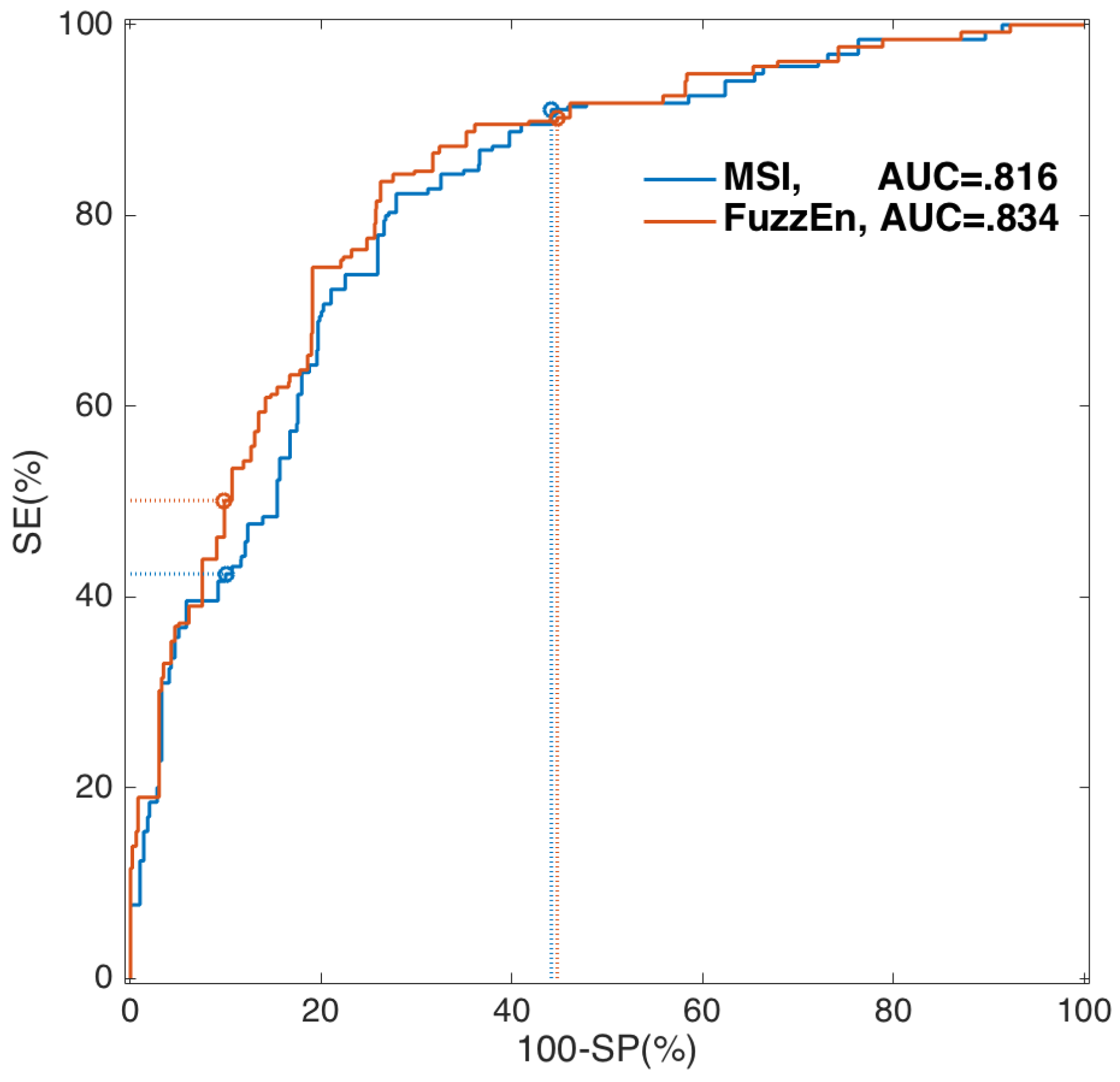
3.3. Optimal Single-Predictor Classifier

The results for the optimal single-predictor SVM classifier evaluated using a LOPCV scheme are reported in Table 3. Entropy measures of regularity produce the best results (minimum BER) and show that balanced SE/SP sensitivities are possible with values for FuzzEn above 80%/75%, respectively. Since the SVMs in the cross-validation loop were optimized in terms of BER, SE/SP values are in general balanced for all predictors. This produces much larger NPVs than PPV, since the proportion of successful shocks in our dataset is roughly 25%/75%. These values are similar to those in most shock outcome prediction studies; for instance, Ristangno et al. [12] report prevalence of 26%/74% in a very large multicenter clinical study on shock outcome prediction. Other optimization criteria can be implemented in the CV loop; for instance, using the weighted F-score ( F β ) for either the positive or negative classes would give preponderance to either one of the four measures [53,54]. In any case, entropy measures of regularity have shown the largest predictive power, both globally (ROC curve analysis) or for a particular optimization criterion (BER).

4. Discussion and Conclusions

The main motivation of the present study stems from the recent success of several indices based on non-linear dynamics for the prediction of VF defibrillation success during OHCA [21,29,30]. These indices convey important information on the metabolic state of the myocardium and on the different phases of VF [21]. We therefore hypothesized that appropriately-chosen entropy features would be an efficient way to quantify the underlying non-linear dynamics of VF. Special focus has been put on the thorough characterization and parametrization of the entropy measures. Four of the six analyzed features were conveniently adapted to encompass VF amplitude information and were shown to be at least as effective in shock outcome prediction as the most elaborate predictors described to date [23,25,26]. This indicates that quantitative entropy measures may be an adequate tool to characterize the non-linear dynamics of the VF waveform.
Our results for the regularity entropy measures confirm our hypothesis. As shown in Figure 2, SampEn, FuzzEn and ApEn (for sufficiently large values of r) have significantly higher values for VF amenable to defibrillation. All of these entropies decrease as m and r increase, since for larger values of these parameters, the probabilities of matches among patterns increase [38]. This also explains the behavior of ApEn for small values of r, because in this case, self-matches are more important, and ϕ m ( r ) can no longer be regarded as an accurate estimation of the conditional probability of a match [46]. The introduction of a soft boundary to define a match improves entropy estimates, particularly for small values of r [31,41]. For low r, not only is ApEn ill-conditioned, but also SampEn may not be computable due to the low number of matches, especially if N is low [41]. This was not the case in our data; however, differences in the qualitative behavior between SampEn and FuzzEn are larger for small r. In fact, for m = 1 , SampEn presents larger values than for m = 2 , 3 . It is noteworthy that FuzzEn depends on the additional parameter n, the gradient of the boundary of the exponential function in D i j m ( n , r ) . Our preliminary experiments showed that the choice of n was not key for shock success prediction; differences in BER were below 0.5 points; consequently, the initial choice of n = 2 was used in this paper.
Predictability entropy measures also showed a consistent behavior in terms of m, ξ or Γ / ξ (Figure 3). However, statistically-significant differences between successful and unsuccessful shocks were only obtained for MConEn. In fact, MConEn was the only symbolic entropy that encoded amplitude information. Some authors have also incorporated amplitude information into entropy measures, particularly in applications where amplitude was relevant to describe time series’ dynamics [55,56]. VF shock outcome prediction exemplifies this type of application, given the strong correlation between VF amplitude, the metabolic state of the heart and its amenability to defibrillation [19]. Entropy measures suitably modified to incorporate amplitude information (ApEn, SampEn, FuzzEn and MConEn) yielded much better shock outcome prediction results than those that exclusively quantified the regularity or predictability of VF (PerEn and ConEn). Moreover, in an additional experiment, where r was normalized by the standard deviation of the data, BER values for regularity-based entropies were around 0.4. It is important to underline that most VF shock outcome predictability indices, including those derived from non-linear dynamics, are amplitude dependent. For instance, MSI and LAC are respectively proportional to VF-amplitude or its square (see Equations (4) and (6)). Non-linear indices insensitive to VF amplitude, such as those based on detrended fluctuation analysis [29] or ApEn estimates for standardized r values [24], report SE/SP values around 60%, in line with our results.
The entropy indices described in this study produced better shock outcome prediction results than the classical predictors. Entropy measures quantify the regularity of the time series by comparing adjacent patterns in different embedding dimensions and convey important information on the self-similarity of the VF waveform. Thus, our approach based on entropy features for the joint quantification of VF amplitude and VF non-linear dynamics is a promising tool to optimize treatment in OHCA. As shown in Table 3, the BER for the best entropy predictor (FuzzEn) was 2.4 points higher than that of the best classical predictor (MSI), which means a combined increase of around five points in SE and SP. There is currently contradictory evidence on the benefits of combining features for shock outcome prediction, with studies showing increases of up to six points in BER for combinations of 3–10 features [57,58] and studies showing no increase in accuracy [23,26]. In a recent study with a large cohort of 1617 patients and 3828 shocks, He et al. [26] found no benefits in combining features and showed the strong correlation among features, such as MdS, AMSA, PPA or energy. Those results confirmed the importance of VF amplitude in shock outcome prediction, since all of those features are proportional to VF amplitude or its square. However, our results suggest that there is information to gain from a combined amplitude and regularity analysis of VF. FuzzEn showed a decrease in BER of 3–5 points with respect to PPA, MdS and/or AMSA. Most likely, shock outcome prediction could be improved by incorporating additional information, such as the relative changes in the predictors between consecutive shocks [59], or other clinical variables, such as end tidal CO2 levels [58].
Furthermore, it is noteworthy that for this study, the optimal working point was defined for a balanced SE/SP combination; consequently, optimization was based on minimizing the BER. However, depending on the clinical setting, different cutoff points could be of interest, for instance to increase confidence on defibrillation success or failure [12,25]. These values are reported in Table 4 for FuzzEn, which shows that in our OHCA data, a threshold of FuzzEn > 0 . 80 could be used to predict defibrillation success with a probability above 89% (PPV), while a threshold of FuzzEn < 0 . 21 predicts defibrillation failure with a probability above 96% (NPV). These thresholds are important should FuzzEn be used clinically in a prospective study, particularly to decide when to continue compressions instead of shocking VF, with the objective of avoiding futile shocks and longer pauses in chest compressions. Prospective studies in which shock outcome predictors, such as AMSA slope or the signal integral [12,60], are used to decide the most adequate therapy for VF are currently planned, thanks to the large body of evidence accumulated in retrospective studies of large patient cohorts [12,26].
The present study has some limitations. First, the results are based on the retrospective analysis of data, and a prospective study would be needed to confirm the benefits of using entropy-based waveform analysis to improve VF therapy on OHCA patients; second, patient outcome data were missing in many of the cases, so the prediction of survival and survival with good neurological outcome based on entropy could not be assessed; finally, the cohort of patients was comparable or larger than that of many studies addressing shock outcome prediction [24,25,57,58], but still limited to draw conclusive evidence on the benefits of using entropy measures to guide VF therapy during OHCA. Our results should be confirmed on data from larger and independent patient cohorts.

Acknowledgments

This work received financial support from Spanish Ministerio de Economía y Competitividad, projects TEC2013-31928 and TEC2014-52250-R, and jointly with the Fondo Europeo de Desarrollo Regional (FEDER), project TEC2015-64678-R; from Junta de Comunidades de Castilla La Mancha, project PPII-2014-026-P; and from UPV/EHU through the grant PIF15/190 and through its research unit UFI11/16.

Author Contributions

Daniel Alonso and Karlos Ibarguren gathered the data from the defibrillators, the clinical data associated with the patients and contributed to the annotation of the datasets. Unai Irusta, Beatriz Chicote, Iraia Isasi and Elisabete Aramendi conceived of and designed the study and participated in the annotation of the data. Beatriz Chicote programmed the experiments, and Unai Irusta supervised the study. Raúl Alcaraz and José Joaquín Rieta conceived of and conducted the experiments on the entropy predictors. Beatriz Chicote, Unai Irusta and Raúl Alcaraz wrote the manuscript, and Elisabete Aramendi, José Joaquín Rieta, Iraia Isasi, Daniel Alonso and Karlos Ibarguren reviewed the manuscript and contributed to the final version. All authors read and approved the final version of the manuscript.

Conflicts of Interest

The authors declare no conflict of interest.

References

  1. Berdowski, J.; Berg, R.A.; Tijssen, J.G.P.; Koster, R.W. Global incidences of out-of-hospital cardiac arrest and survival rates: Systematic review of 67 prospective studies. Resuscitation 2010, 81, 1479–1487. [Google Scholar] [CrossRef] [PubMed]
  2. Rubart, M.; Zipes, D.P. Mechanisms of sudden cardiac death. J. Clin. Investig. 2005, 115, 2305–2315. [Google Scholar] [CrossRef] [PubMed]
  3. Zoll, P.M. Resuscitation of the heart in ventricular standstill by external electric stimulation. New Engl. J. Med. 1952, 247, 768–771. [Google Scholar] [CrossRef] [PubMed]
  4. Perkins, G.D.; Handley, A.J.; Koster, R.W.; Castrén, M.; Smyth, M.A.; Olasveengen, T.; Monsieurs, K.G.; Raffay, V.; Gräsner, J.T.; Wenzel, V.; et al. European Resuscitation Council Guidelines for Resuscitation 2015: Section 2. Adult basic life support and automated external defibrillation. Resuscitation 2015, 95, 81–99. [Google Scholar] [CrossRef] [PubMed]
  5. Kleinman, M.E.; Brennan, E.E.; Goldberger, Z.D.; Swor, R.A.; Terry, M.; Bobrow, B.J.; Gazmuri, R.J.; Travers, A.H.; Rea, T. Part 5: Adult Basic Life Support and Cardiopulmonary Resuscitation Quality: 2015 American Heart Association Guidelines Update for Cardiopulmonary Resuscitation and Emergency Cardiovascular Care. Circulation 2015, 132, S414–S435. [Google Scholar] [CrossRef] [PubMed]
  6. Rudikoff, M.T.; Maughan, W.L.; Effron, M.; Freund, P.; Weisfeldt, M.L. Mechanisms of blood flow during cardiopulmonary resuscitation. Circulation 1980, 61, 345–352. [Google Scholar] [CrossRef] [PubMed]
  7. Monsieurs, K.G.; Nolan, J.P.; Bossaert, L.L.; Greif, R.; Maconochie, I.K.; Nikolaou, N.I.; Perkins, G.D.; Soar, J.; Truhlář, A.; Wyllie, J.; et al. European Resuscitation Council Guidelines for Resuscitation 2015: Section 1. Executive summary. Resuscitation 2015, 95, 1–80. [Google Scholar] [CrossRef] [PubMed]
  8. Neumar, R.W.; Shuster, M.; Callaway, C.W.; Gent, L.M.; Atkins, D.L.; Bhanji, F.; Brooks, S.C.; de Caen, A.R.; Donnino, M.W.; Ferrer, J.M.E.; et al. Part 1: Executive Summary: 2015 American Heart Association Guidelines Update for Cardiopulmonary Resuscitation and Emergency Cardiovascular Care. Circulation 2015, 132, S315–S367. [Google Scholar] [CrossRef] [PubMed]
  9. Ruiz de Gauna, S.; Irusta, U.; Ruiz, J.; Ayala, U.; Aramendi, E.; Eftestøl, T. Rhythm analysis during cardiopulmonary resuscitation: past, present, and future. Biomed. Res. Int. 2014, 2014, 386010. [Google Scholar] [CrossRef] [PubMed]
  10. Irusta, U.; Ruiz, J.; Aramendi, E.; Ruiz de Gauna, S.; Ayala, U.; Alonso, E. A high-temporal resolution algorithm to discriminate shockable from nonshockable rhythms in adults and children. Resuscitation 2012, 83, 1090–1097. [Google Scholar] [CrossRef] [PubMed]
  11. Eftestol, T.; Sunde, K.; Ole Aase, S.; Husoy, J.H.; Steen, P.A. Predicting outcome of defibrillation by spectral characterization and nonparametric classification of ventricular fibrillation in patients with out-of-hospital cardiac arrest. Circulation 2000, 102, 1523–1529. [Google Scholar] [CrossRef] [PubMed]
  12. Ristagno, G.; Mauri, T.; Cesana, G.; Li, Y.; Finzi, A.; Fumagalli, F.; Rossi, G.; Grieco, N.; Migliori, M.; Andreassi, A.; et al. Amplitude spectrum area to guide defibrillation: A validation on 1617 patients with ventricular fibrillation. Circulation 2015, 131, 478–487. [Google Scholar] [CrossRef] [PubMed]
  13. Xie, J.; Weil, M.H.; Sun, S.; Tang, W.; Sato, Y.; Jin, X.; Bisera, J. High-energy defibrillation increases the severity of postresuscitation myocardial dysfunction. Circulation 1997, 96, 683–688. [Google Scholar] [CrossRef] [PubMed]
  14. Cheskes, S.; Schmicker, R.H.; Christenson, J.; Salcido, D.D.; Rea, T.; Powell, J.; Edelson, D.P.; Sell, R.; May, S.; Menegazzi, J.J.; et al. Perishock pause: An independent predictor of survival from out-of-hospital shockable cardiac arrest. Circulation 2011, 124, 58–66. [Google Scholar] [CrossRef] [PubMed]
  15. Weisfeldt, M.L.; Becker, L.B. Resuscitation after cardiac arrest: A 3-phase time-sensitive model. JAMA 2002, 288, 3035–3038. [Google Scholar] [CrossRef] [PubMed]
  16. Reed, M.J.; Clegg, G.R.; Robertson, C.E. Analysing the ventricular fibrillation waveform. Resuscitation 2003, 57, 11–20. [Google Scholar] [CrossRef]
  17. Callaway, C.W.; Menegazzi, J.J. Waveform analysis of ventricular fibrillation to predict defibrillation. Curr. Opin. Crit. Care 2005, 11, 192–199. [Google Scholar] [CrossRef] [PubMed]
  18. Salcido, D.D.; Menegazzi, J.J.; Suffoletto, B.P.; Logue, E.S.; Sherman, L.D. Association of intramyocardial high energy phosphate concentrations with quantitative measures of the ventricular fibrillation electrocardiogram waveform. Resuscitation 2009, 80, 946–950. [Google Scholar] [CrossRef] [PubMed]
  19. Weaver, W.D.; Cobb, L.A.; Dennis, D.; Ray, R.; Hallstrom, A.P.; Copass, M.K. Amplitude of ventricular fibrillation waveform and outcome after cardiac arrest. Ann. Intern. Med. 1985, 102, 53–55. [Google Scholar] [CrossRef] [PubMed]
  20. Callaway, C.W.; Sherman, L.D.; Scheatzle, M.D.; Menegazzi, J.J. Scaling structure of electrocardiographic waveform during prolonged ventricular fibrillation in swine. Pacing Clin. Electrophysiol. 2000, 23, 180–191. [Google Scholar] [CrossRef] [PubMed]
  21. Sherman, L.D.; Rea, T.D.; Waters, J.D.; Menegazzi, J.J.; Callaway, C.W. Logarithm of the absolute correlations of the ECG waveform estimates duration of ventricular fibrillation and predicts successful defibrillation. Resuscitation 2008, 78, 346–354. [Google Scholar] [CrossRef] [PubMed]
  22. Dzwonczyk, R.; Brown, C.G.; Werman, H.A. The median frequency of the ECG during ventricular fibrillation: Its use in an algorithm for estimating the duration of cardiac arrest. IEEE Trans. Biomed. Eng. 1990, 37, 640–646. [Google Scholar] [CrossRef] [PubMed]
  23. Neurauter, A.; Eftestøl, T.; Kramer-Johansen, J.; Abella, B.S.; Sunde, K.; Wenzel, V.; Lindner, K.H.; Eilevstjønn, J.; Myklebust, H.; Steen, P.A.; et al. Prediction of countershock success using single features from multiple ventricular fibrillation frequency bands and feature combinations using neural networks. Resuscitation 2007, 73, 253–263. [Google Scholar] [CrossRef] [PubMed]
  24. Endoh, H.; Hida, S.; Oohashi, S.; Hayashi, Y.; Kinoshita, H.; Honda, T. Prompt prediction of successful defibrillation from 1-s ventricular fibrillation waveform in patients with out-of-hospital sudden cardiac arrest. J. Anesth. 2011, 25, 34–41. [Google Scholar] [CrossRef] [PubMed]
  25. Firoozabadi, R.; Nakagawa, M.; Helfenbein, E.D.; Babaeizadeh, S. Predicting defibrillation success in sudden cardiac arrest patients. J. Electrocardiol. 2013, 46, 473–479. [Google Scholar] [CrossRef] [PubMed]
  26. He, M.; Gong, Y.; Li, Y.; Mauri, T.; Fumagalli, F.; Bozzola, M.; Cesana, G.; Latini, R.; Pesenti, A.; Ristagno, G. Combining multiple ECG features does not improve prediction of defibrillation outcome compared to single features in a large population of out-of-hospital cardiac arrests. Crit. Care 2015, 19. [Google Scholar] [CrossRef] [PubMed]
  27. Marn-Pernat, A.; Weil, M.H.; Tang, W.; Pernat, A.; Bisera, J. Optimizing timing of ventricular defibrillation. Crit. Care Med. 2001, 29, 2360–2365. [Google Scholar] [CrossRef] [PubMed]
  28. Sherman, L.D.; Callaway, C.W.; Menegazzi, J.J. Ventricular fibrillation exhibits dynamical properties and self-similarity. Resuscitation 2000, 47, 163–173. [Google Scholar] [CrossRef]
  29. Lin, L.Y.; Lo, M.T.; Ko, P.C.I.; Lin, C.; Chiang, W.C.; Liu, Y.B.; Hu, K.; Lin, J.L.; Chen, W.J.; Ma, M.H.M. Detrended fluctuation analysis predicts successful defibrillation for out-of-hospital ventricular fibrillation cardiac arrest. Resuscitation 2010, 81, 297–301. [Google Scholar] [CrossRef] [PubMed]
  30. Gong, Y.; Lu, Y.; Zhang, L.; Zhang, H.; Li, Y. Predict Defibrillation Outcome Using Stepping Increment of Poincaree Plot for Out-of-Hospital Ventricular Fibrillation Cardiac Arrest. Biomed. Res. Int. 2015, 2015, 493472. [Google Scholar] [CrossRef] [PubMed]
  31. Chen, W.; Zhuang, J.; Yu, W.; Wang, Z. Measuring complexity using FuzzyEn, ApEn, and SampEn. Med. Eng. Phys. 2009, 31, 61–68. [Google Scholar] [CrossRef] [PubMed]
  32. Li, P.; Liu, C.; Li, K.; Zheng, D.; Liu, C.; Hou, Y. Assessing the complexity of short-term heartbeat interval series by distribution entropy. Med. Biol. Eng. Comput. 2015, 53, 77–87. [Google Scholar] [CrossRef] [PubMed]
  33. Borowska, M. Entropy-based algorithms in the analysis of biomedical signals. Stud. Log. Gramm. Rhetor. 2015, 43, 21–32. [Google Scholar] [CrossRef]
  34. Faust, O.; Bairy, M.G. Nonlinear analysis of physiological signals: A review. J. Mech. Med. Biol. 2012, 12, 124005. [Google Scholar] [CrossRef]
  35. Ibarguren, K.; Unanue, J.M.; Alonso, D.; Vaqueriza, I.; Irusta, U.; Aramendi, E.; Chicote, B. Difference in survival from pre-hospital cardiac arrest between cities and villages in the Basque Autonomous Community. Resuscitation 2015, 96. [Google Scholar] [CrossRef]
  36. Higuchi, T. Approach to an irregular time series on the basis of the fractal theory. Physica D 1988, 31, 277–283. [Google Scholar] [CrossRef]
  37. Sherman, L.D.; Flagg, A.; Callaway, C.W.; Menegazzi, J.J.; Hsieh, M. Angular velocity: A new method to improve prediction of ventricular fibrillation duration. Resuscitation 2004, 60, 79–90. [Google Scholar] [CrossRef] [PubMed]
  38. Pincus, S.M. Approximate entropy as a measure of system complexity. Proc. Natl. Acad. Sci. USA 1991, 88, 2297–2301. [Google Scholar] [CrossRef] [PubMed]
  39. Amigó, J.M.; Keller, K.; Unakafova, V.A. Ordinal symbolic analysis and its application to biomedical recordings. Philos. Trans. A Math. Phys. Eng. Sci. 2015, 373. [Google Scholar] [CrossRef] [PubMed]
  40. Richman, J.S.; Moorman, J.R. Physiological time-series analysis using approximate entropy and sample entropy. Am. J. Physiol. Heart Circ. Physiol. 2000, 278, H2039–H2049. [Google Scholar] [PubMed]
  41. Chen, W.; Wang, Z.; Xie, H.; Yu, W. Characterization of surface EMG signal based on fuzzy entropy. IEEE. Trans. Neural Syst. Rehabil. Eng. 2007, 15, 266–272. [Google Scholar] [CrossRef] [PubMed]
  42. Bandt, C.; Pompe, B. Permutation entropy: A natural complexity measure for time series. Phys. Rev. Lett. 2002, 88, 174102. [Google Scholar] [CrossRef] [PubMed]
  43. Porta, A.; Guzzetti, S.; Montano, N.; Furlan, R.; Pagani, M.; Malliani, A.; Cerutti, S. Entropy, entropy rate, and pattern classification as tools to typify complexity in short heart period variability series. IEEE Trans. Biomed. Eng. 2001, 48, 1282–1291. [Google Scholar] [CrossRef] [PubMed]
  44. Lu, S.; Chen, X.; Kanters, J.K.; Solomon, I.C.; Chon, K.H. Automatic selection of the threshold value R for approximate entropy. IEEE. Trans. Biomed. Eng. 2008, 55, 1966–1972. [Google Scholar] [PubMed]
  45. Alcaraz, R.; Abásolo, D.; Hornero, R.; Rieta, J.J. Optimal parameters study for sample entropy-based atrial fibrillation organization analysis. Comput. Methods Programs Biomed. 2010, 99, 124–132. [Google Scholar] [CrossRef] [PubMed] [Green Version]
  46. Singh, A.; Saini, B.S.; Singh, D. An alternative approach to approximate entropy threshold value (r) selection: Application to heart rate variability and systolic blood pressure variability under postural challenge. Med. Biol. Eng. Comput. 2016, 54, 723–732. [Google Scholar] [CrossRef] [PubMed]
  47. Zanin, M.; Zunino, L.; Rosso, O.A.; Papo, D. Permutation Entropy and Its Main Biomedical and Econophysics Applications: A Review. Entropy 2012, 14, 1553–1577. [Google Scholar] [CrossRef]
  48. Porta, A.; Baselli, G.; Liberati, D.; Montano, N.; Cogliati, C.; Gnecchi-Ruscone, T.; Malliani, A.; Cerutti, S. Measuring regularity by means of a corrected conditional entropy in sympathetic outflow. Biol. Cybern. 1998, 78, 71–78. [Google Scholar] [CrossRef] [PubMed]
  49. Zou, K.H.; O’Malley, A.J.; Mauri, L. Receiver-operating characteristic analysis for evaluating diagnostic tests and predictive models. Circulation 2007, 115, 654–657. [Google Scholar] [CrossRef] [PubMed]
  50. Ben-Hur, A.; Weston, J. A user’s guide to support vector machines. Methods Mol. Biol. 2010, 609, 223–239. [Google Scholar] [PubMed]
  51. Khandoker, A.H.; Gubbi, J.; Palaniswami, M. Automated scoring of obstructive sleep apnea and hypopnea events using short-term electrocardiogram recordings. IEEE Trans. Inform. Technol. Biomed. 2009, 13, 1057–1067. [Google Scholar] [CrossRef] [PubMed]
  52. Lillo-Castellano, J.M.; Mora-Jiménez, I.; Santiago-Mozos, R.; Chavarría-Asso, F.; Cano-González, A.; García-Alberola, A.; Rojo-Álvarez, J.L. Symmetrical compression distance for arrhythmia discrimination in cloud-based big-data services. IEEE J. Biomed. Health Inform. 2015, 19, 1253–1263. [Google Scholar] [CrossRef] [PubMed]
  53. Musicant, D.R.; Kumar, V.; Ozgur, A. Optimizing F-Measure with Support Vector Machines. In Proceedings of the FLAIRS Conference, St. Augustine, FL, USA, 12–14 May 2003; pp. 356–360.
  54. Sokolova, M.; Japkowicz, N.; Szpakowicz, S. Beyond accuracy, F-score and ROC: A family of discriminant measures for performance evaluation. In AI 2006: Advances in Artificial Intelligence; Springer: Berlin/Heidelberg, Germany, 2006; pp. 1015–1021. [Google Scholar]
  55. Xiao-Feng, L.; Yue, W. Fine-grained permutation entropy as a measure of natural complexity for time series. Chin. Phys. B 2009, 18. [Google Scholar] [CrossRef]
  56. Fadlallah, B.; Chen, B.; Keil, A.; Príncipe, J. Weighted-permutation entropy: A complexity measure for time series incorporating amplitude information. Phys. Rev. E 2013, 87, 022911. [Google Scholar] [CrossRef] [PubMed]
  57. Howe, A.; Escalona, O.J.; di Maio, R.; Massot, B.; Cromie, N.A.; Darragh, K.M.; Adgey, J.; McEneaney, D.J. A support vector machine for predicting defibrillation outcomes from waveform metrics. Resuscitation 2014, 85, 343–349. [Google Scholar] [CrossRef] [PubMed]
  58. Shandilya, S.; Ward, K.; Kurz, M.; Najarian, K. Non-linear dynamical signal characterization for prediction of defibrillation success through machine learning. BMC Med. Inform. Decis. Mak. 2012, 12. [Google Scholar] [CrossRef] [PubMed]
  59. He, M.; Lu, Y.; Zhang, L.; Zhang, H.; Gong, Y.; Li, Y. Combining Amplitude Spectrum Area with Previous Shock Information Using Neural Networks Improves Prediction Performance of Defibrillation Outcome for Subsequent Shocks in Out-Of-Hospital Cardiac Arrest Patients. PLoS ONE 2016, 11, e0149115. [Google Scholar] [CrossRef] [PubMed]
  60. Wu, X.; Bisera, J.; Tang, W. Signal integral for optimizing the timing of defibrillation. Resuscitation 2013, 84, 1704–1707. [Google Scholar] [CrossRef] [PubMed]
Figure 1. Three shocks in which ventricular fibrillation (VF) converted to an organized rhythm (ORG) (a); again to VF (b); and to asystole (ASY) (c). The resulting rhythm is observed after the shock, which in all cases is shown after about 10 s (the ECG signal is lost during the shock). Chest compressions were given during the shaded intervals, and the resulting CPR artifact is observed in the ECG. In addition, the 5- s VF pre-shock analysis segment used to compute the predictors is highlighted.
Entropy 18 00313 g001
Figure 2. Median values of the regularity-based entropies (y-axes) for the successful and unsuccessful shocks. The values are shown as a function of the fixed amplitude threshold r and in different traces for different values of m. (a) ApEn; (b) SampEn; (c) FuzzEn.
Entropy 18 00313 g002
Figure 3. Median values of the predictability-based entropies (y-axes) for the successful and unsuccessful shocks. The values are shown as a function of the adjustable parameters for each entropy. (a) PerEn; (b) ConEn; (c) MConEn.
Entropy 18 00313 g003
Figure 4. Box plots of the predictors for the successful and unsuccessful shocks; the y-axes represent the values of the predictors. All predictors showed significant differences in the distributions, except for PerEn and ConEn. The values also show the ranges for the different predictors. (a) Classical predictors; (b) Entropy based predictors.
Entropy 18 00313 g004
Figure 5. ROC curves and significant cutoffs for the best classical and entropy predictor.
Entropy 18 00313 g005
Table 1. Optimal input parameters selected for the entropy measures. ApEn, approximate entropy; FuzzEn, fuzzy entropy; SampEn, sample entropy; PerEn, permutation entropy; ConEn, conditional entropy; MConEn, modified version of ConEn.
MeasureOptimal Input Parameters
ApEn m = 1 and r = 55 μ V
SampEn m = 1 and r = 50 μ V
FuzzEn m = 3 and r = 80 μ V
PerEn m = 6
ConEn m = 2 and ξ = 10
MConEn m = 2 and Γ / ξ = 300 μ V
Table 2. ROC curve analysis for the predictors. PPA, peak-to-peak amplitude; MdS, median slope; AMSA, amplitude spectrum area; MSI, median length of the stepping increment; ScE, scaling exponent; LAC, logarithm of the absolute correlation; SE, sensitivity; SP, specificity.
PredictorAUCSE (%) aSP (%) b
PPA0.80441.250.6
MdS0.81541.956.3
AMSA0.80643.952.3
MSI0.81642.455.9
ScE0.77836.543.4
LAC0.72625.934.2
ApEn0.81342.753.5
SampEn0.81340.453.5
FuzzEn0.83450.155.2
PerEn0.55013.112.8
ConEn0.63615.519.4
MConEn0.82046.755.4
a for SP = 90%, b for SE = 90%.
Table 3. Classification results for the optimal SVM classifiers evaluated using an leave one patient out cross-validation (LOPCV) scheme. BER, balanced error rate; PPV, positive predictive value; NPV, negative predictive value.
PredictorBERSE (%)SP (%)PPV (%)NPV (%)
PPA0.24780.470.248.091.2
MdS0.23979.472.850.091.2
AMSA0.26774.871.847.689.2
MSI0.23880.472.149.791.5
ScE0.27383.262.243.091.5
LAC0.33075.758.338.487.5
ApEn0.22081.374.752.492.1
SampEn0.21881.375.052.792.1
FuzzEn0.21480.476.954.492.0
PerEn0.47537.467.628.475.9
ConEn0.43643.069.932.978.1
MConEn0.23085.068.948.493.1
Table 4. Thresholds for defibrillation success/failure based on FuzzEn computed for n = 2 , m = 3 and r = 80 μ V . The values are based on the ROC curve analysis (see Figure 5).
ThresholdSE (%)SP (%)PPV (%)NPV (%)
Defibrillation Failure
   FuzzEn < 0.21 98.521.139.496.3
   FuzzEn < 0.29 95.634.743.293.9
   FuzzEn < 0.38 90.355.251.291.6
Defibrillation Success
   FuzzEn > 0.80 19.098.889.270.1
   FuzzEn > 0.67 36.995.380.474.4
   FuzzEn > 0.62 50.190.272.677.7

