Mechanical Fault Diagnosis of High Voltage Circuit Breakers with Unknown Fault Type Using Hybrid Classifier Based on LMD and Time Segmentation Energy Entropy

Abstract

In order to improve the identification accuracy of the high voltage circuit breakers’ (HVCBs) mechanical fault types without training samples, a novel mechanical fault diagnosis method of HVCBs using a hybrid classifier constructed with Support Vector Data Description (SVDD) and fuzzy c-means (FCM) clustering method based on Local Mean Decomposition (LMD) and time segmentation energy entropy (TSEE) is proposed. Firstly, LMD is used to decompose nonlinear and non-stationary vibration signals of HVCBs into a series of product functions (PFs). Secondly, TSEE is chosen as feature vectors with the superiority of energy entropy and characteristics of time-delay faults of HVCBs. Then, SVDD trained with normal samples is applied to judge mechanical faults of HVCBs. If the mechanical fault is confirmed, the new fault sample and all known fault samples are clustered by FCM with the cluster number of known fault types. Finally, another SVDD trained by the specific fault samples is used to judge whether the fault sample belongs to an unknown type or not. The results of experiments carried on a real SF₆ HVCB validate that the proposed fault-detection method is effective for the known faults with training samples and unknown faults without training samples.

1. Introduction

As the indispensable equipment in power systems, high voltage circuit breakers (HVCBs) are very important for ensuring the power supply reliability and safe operation of the power system. Mechanical faults are the main reasons that affect the reliability of HVCBs [1,2,3,4,5]. It is therefore necessary to carry out the research on the diagnosis method of HVCB mechanical faults in order to ensure the safe and stable running of the power system.

The typical mechanical fault diagnosis method for HVCBs includes scheduled maintenance and condition-based maintenance. The scheduled maintenance is not only time consuming and laborious, but also leads to excessive operations and overhauls. It may result in needless intervention and even cause faults of HVCBs during the maintenance. The fault diagnosis results of scheduled maintenance are estimated by experience of maintenance workers [6,7]. In order to avoid the limitation of scheduled maintenance for HVCBs, the condition-based maintenance has developed in recent years. Condition-based maintenance is carried out by analyzing the on-line monitoring normal operating data without additional HVCB operation. Thus, condition monitoring can not only avoid the inconvenience caused by scheduled maintenance, but can also reduce the damage of HVCBs by excessive maintenance.

The automatic fault diagnosis accuracy is the pivotal issue of condition-based maintenance to ensure the operational reliability of a power system. Most of the studies on automatic fault diagnosis method have not considered the limitation of fault samples [8,9,10,11,12,13,14]. They only choose normal samples and several known types of fault samples as training samples to train multi-classifiers and carry out fault diagnosis. However, in the real power system, the operation of HVCBs is rare. It is difficult to acquire enough fault samples with all fault types. Furthermore, the objective of the traditional method is to achieve the highest comprehensive recognition accuracy of the normal state and all types of faults. It can thus easily misidentify the fault types without training samples as normal samples. Here, we define the known fault types as the fault types which have occurred and been recorded in a power system, or can be obtained in a laboratory environment. Unknown fault types are the fault types which have not happened in a power system, or cannot be obtained by experiment for reasons of cost, etc. Even if the fault state can be detected, it is still easy to misidentify the unknown fault types as known fault types, which may affect the targeted maintenance of HVCBs [5]. Therefore, the traditional multi-classifiers are not satisfied by the specific circumstance requirement of HVCB fault diagnosis.

At present, the commonly used fault diagnosis methods mainly include the observer-based method [15,16,17], vibration analysis method [11,12,13,14], etc. The observer-based method is often used to diagnose the nonlinear systems with uncertain parameters. It has been widely applied in fault diagnosis fields such as the fault diagnosis of wind turbines [15]. However, because the operation of HVCBs is rare, it is very difficult to acquire enough fault samples and construct reliable mathematical models for HVCB fault diagnosis. Vibration analysis is an effective approach to fault diagnosis [5,18]. Vibration signals, generated during the opening/closing operation of HVCBs, contain important information about the mechanical state. Therefore, vibration analysis has garnered more and more attention in HVCB fault diagnosis [14,19]. The signal processing method of vibration signals is the foundation of mechanical fault feature extraction. The existing signal processing methods such as short-time Fourier transform (STFT), wavelet packet transform (WPT) [20,21,22] and empirical mode decomposition (EMD) [14] are often used to extract the fault feature vector. However, these methods also have a few limitations. STFT uses a time-frequency window function with fixed width to analyze signals in the time and frequency domains, so the ability of time-frequency characterizing is limited. Compared with STFT, WPT has better time-frequency analysis performance [21,22], but its wavelet basis function needs to be predefined for each component, and final results are influenced greatly by the wavelet basis function [10,11]. EMD is a self-adaptive time-frequency analysis method for nonlinear and non-stationary signals. However, the limitations as end effect, mode confusion and high time consumption affect its application [12,13]. Local Mean Decomposition (LMD), as a new self-adaptive time-frequency method, was developed by Smith in 2005 [23]. The LMD method can adaptively decompose a multi-component amplitude-modulated and frequency-modulated (AM–FM) signal into a series of product functions (PFs). Each PF is the product of an envelope signal and a purely frequency-modulated signal. The instantaneous frequencies can be derived from the purely frequency-modulated signal [23,24]. Thus, the LMD method has been widely applied in the rotating machine fault diagnosis field in recent years [12,13]. However, there has not been any application of HVCBs in the fault diagnosis field. As with the vibration signals of rotating machine, vibration signals of HVCBs also show AM-FM features, so the LMD method is suitable for processing the vibration signal of HVCBs. Although the LMD method is ostensibly similar to the EMD method, the comparison results show that LMD is better than EMD in some aspects, such as greater ability to mitigate end effect, less iteration, fewer decomposed components, and so on [10,12].

After processing the vibration signals of HVCBs, the main task is to extract an effective feature from the obtained components. The energy distribution of the different states of HVCB vibration signals has significant discrepancies. Energy entropy can quantitatively describe the complex energy distribution in the time-frequency area [25]. Therefore, it is effective to choose energy entropy of each PF component as the feature vector for most mechanical faults. However, for the time-delay faults of HVCBs such as jam fault of the iron core, it will be difficult to accurately distinguish fault samples from normal samples [11,14]. Considering that the energy distribution of time-delay faults has an apparent time delay, the time domain segmentation energy entropy (TSEE) used as the feature vector could significantly improve the diagnosis ability for time-delay faults.

After the extraction of feature vectors, a classifier is used to automatically identify the fault types of HVCBs. Support vector machine (SVM) [25,26], back propagation neural network (BPNN) [27,28] and other traditional multi-classification methods have made a great contribution to fault identification, but because of the aforementioned drawbacks, traditional multi-classification methods cannot meet the high reliability requirement of an electrical power system. One-class classifiers can complete the training only using the normal state samples which are relatively easy to obtain. It is very satisfied for the high reliability applications [5]. Support Vector Data Description (SVDD) was proposed by Tax [29]. It has the advantages of faster training and decision, lower requirement for training samples, strong anti-noise ability and being suitable for small sample. SVDD has been successfully applied to the field of fault detection. For new fault types without training samples, SVDD can identify them as fault samples, though it cannot determine whether the fault type is new or not. Fuzzy c-means (FCM) cluster method [30,31] can divide similar samples into the same class, and it is not dependent on the training samples. It is thus very useful to analyze the unknown fault sample without training samples.

The main contribution of this paper is to propose a novel mechanical fault diagnosis method of HVCBs based on LMD, TSEE and the hybrid classifier. This method can solve the problem of traditional research easily misidentifying the fault types without training samples (unknown fault types) as normal samples or known fault types. Firstly, LMD is used to decompose vibration signals of HVCBs into a series of PFs. Secondly, TSEEs are extracted to construct feature vectors for describing the energy distribution of HVCB vibration signals in the time and frequency domain. Then, a SVDD trained with normal samples is used to distinguish the normal and fault states of HVCBs. If a mechanical fault is confirmed, the fault sample and all samples with known fault types are clustered by the FCM method with the number of known fault types. According to the clustering results, another SVDD trained with a type of known fault sample is used to judge whether the fault sample belongs to a new type or not, and the final recognition results are determined. The experiment results are used to prove the advantage of the new method.

2. Vibration Signal Processing through LMD Method

2.1. Local Mean Decomposition (LMD) Analysis Method

In order to extract effective information about mechanical state from vibration signals, a multi-component signal is decomposed automatically into a set of mono-component signals which are called product functions (PFs) using the LMD method. For any signal $x(t)$, it can be decomposed by the following steps [23].

(1)

Determine all local extreme $p_i$ of the signal $x(t)$, then calculate the mean value of two successive extreme $p_i$ and $p_{i+1}$. Therefore, the $i\mathrm{th}$ mean value $m_i$ can be obtained by:

$$m_i=\frac{p_i+p_{i+1}}{2},$$

(1)

All mean values $m_i$ calculated by Equation (1) are connected by straight lines first. Then, the local means are smoothed using moving averaging. The first local mean function $m_{11}(t)$ which is smoothly varying continuous is obtained.

(2)

The $i\mathrm{th}$ envelope estimate $a_i$ can be calculated by:

$$a_i=\frac{\left|p_i-p_{i+1}\right|}{2},$$

(2)

(3)

The first envelope function $a_{11}(t)$ can be obtained by the same smoothing method as the local means. The local mean function $m_{11}(t)$ is separated from original signal $x(t)$, and the resulting signal denoted as $h_{11}(t)$ can be derived by:

$$h_{11}(t)=x(t)-m_{11}(t),$$

(3)

(4)

In order to achieve the demodulation of $h_{11}(t)$, $h_{11}(t)$ is divided by the envelope function $a_{11}(t)$.

$$s_{11}(t)=h_{11}(t)/a_{11}(t),$$

(4)

$s_{11}(t)$ is a purely frequency-modulated signal and the procedure should be stopped. Otherwise, $s_{11}(t)$ should be regarded as the signal to be decomposed, and the steps (1)–(4) are repeated q times until the condition $a_{1(q+1)}(t)=1$ is satisfied. At this point, $s_{1q}(t)$ is a purely frequency-modulated signal. Therefore,

$$\{\begin{array}{ccc}{h}_{11}(t)\hfill & \hfill =\hfill & x(t)-m_{11}(t)\hfill \\ h_{12}(t)\hfill & \hfill =\hfill & s_{11}(t)-m_{12}(t)\hfill \\ & \hfill ⋮\hfill & \\ h_{1q}(t)\hfill & \hfill =\hfill & s_{1(q-1)}(t)-m_{1q}(t)\hfill \end{array},$$

(5)

in which

$$\{\begin{array}{ccc}{s}_{11}(t)\hfill & \hfill =\hfill & h_{11}(t)/a_{11}(t)\hfill \\ s_{12}(t)\hfill & \hfill =\hfill & h_{12}(t)/a_{12}(t)\hfill \\ & \hfill ⋮\hfill & \\ s_{1q}(t)\hfill & \hfill =\hfill & h_{1q}(t)/a_{1q}(t)\hfill \end{array},$$

(6)

When the following condition is satisfied, the iterations should be stopped.

$$\underset{q\to \infty }{\lim }{a}_{1(q+1)}(t)=1,$$

(7)

However, for practical application, it is too strict to satisfy this criterion. An additional stop condition can be set as $a_{1(q+1)}\in [1-\Delta e,1+\Delta e]$, which will contribute to reducing the number of iterations, improving the speed of computing and mitigating the impact of end effect, where $\Delta e$ is an established variable.

(5)

The envelope signal $a_1(t)$ of the first product function $P{F}_1(t)$ is obtained by Equation (8).

$$a_1(t)=a_{11}(t)a_{12}(t)\cdots a_{1q}(t)={\displaystyle \prod _{b=1}^q{a}_{1b}(t)},$$

(8)

The instantaneous amplitude of $P{F}_1(t)$ is the envelope signal $a_1(t)$. The $P{F}_1(t)$ is structured by the envelope signal $a_1(t)$ and the purely frequency-modulated signal $s_{1q}\left(t\right)$.

$$P{F}_1(t)=a_1(t)s_{1q}(t),$$

(9)

Actually, $P{F}_1(t)$ is a mono-component AM-FM signal. Its instantaneous frequency can be obtained by Equation (10)

$$f_1(t)=\frac{1}{2\pi }\frac{d[\arccos (s_{1q}(t))]}{dt},$$

(10)

(6)

Then, $P{F}_1(t)$ is separated from the original signal $x(t)$ and a new signal $u_1\left(t\right)$ is obtained. Take $u_1\left(t\right)$ as a signal to be decomposed and repeat the procedure $d$ times until $u_d(t)$ is a constant or a monotonic function.

$$\{\begin{array}{ccc}{u}_1(t)\hfill & \hfill =\hfill & x(t)-P{F}_1(t)\hfill \\ u_2(t)\hfill & \hfill =\hfill & u_1(t)-P{F}_2(t)\hfill \\ & \hfill ⋮\hfill & \\ u_d(t)\hfill & \hfill =\hfill & u_{d-1}(t)-P{F}_d(t)\hfill \end{array},$$

(11)

Consequently, the original signal $x(t)$ can be reconstructed by all PF components and a residue $u_d(t)$ as Equation (12).

$$x(t)={\displaystyle \sum _{m=1}^{d}P{F}_m(t)+u_d(t)},$$

(12)

where $d$ is the number of the derived PF components.

According to the results of LMD, a multi-component signal can be decomposed into a set of mono-component PF components and a residue. The PF components contain different frequency bands ranging from high to low. After the decomposition of original signals, the results can clearly reflect the intrinsic information and local characteristics of the signal, which will contribute to diagnosing the mechanical faults of HVCBs.

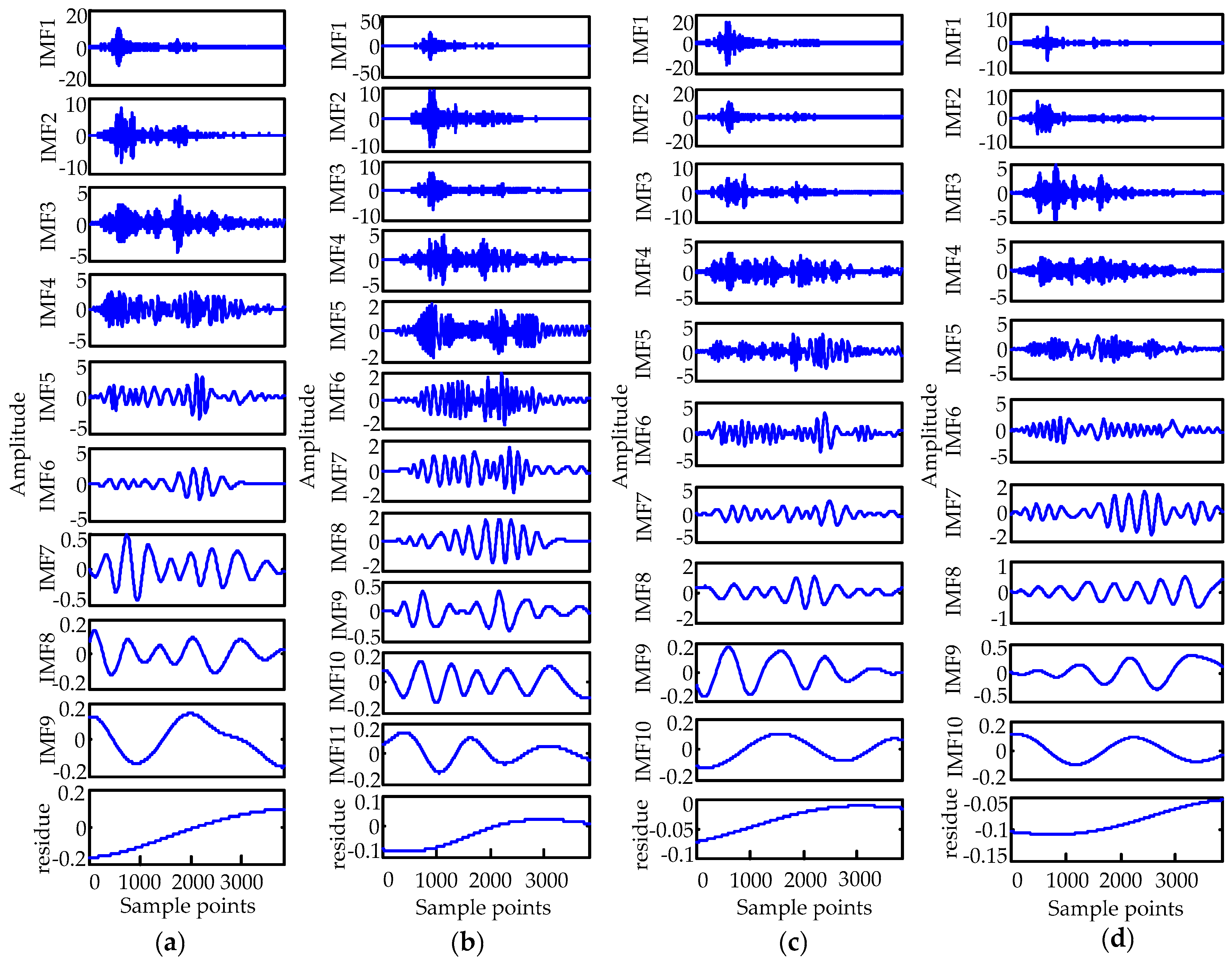
2.2. Analysis of the Results Obtained by the LMD Method

Three types of mechanical fault signals were collected in a field experiment on a real HVCB: (1) jam fault of the iron core (fault type I); (2) lack of mechanical lubrication (fault type II); (3) base screw looseness (fault type III). Figure 1 shows the waveform of normal signal and three types of fault signals. The sampling time of each sample is 150 ms and the sampling frequency is 25.6 kS/s, so each sample contains 3840 sampling points. The corresponding starting times of four types of signals are denoted as $t_1,t_2,t_3$ and $t_4$ with the dashed lines in the figure.

As shown in Figure 1, the starting time of fault type I and fault type II lags behind the normal signal in different degrees. The maximum amplitude of fault type III is less than the other types of signals; and the change of amplitude of fault type III is small in sampling time.

The four types of vibration signals are decomposed using LMD and EMD separately. The results are shown in Figure 2 and Figure 3. In Figure 2 and Figure 3, each component contains 3840 sample points.

From Figure 2 and Figure 3, we can find that different vibration signals have different numbers of components. For the same signal, components obtained by LMD are fewer than EMD. This advantage can guarantee that the feature information will not be divided into a few adjacent decomposition levels which contain similar information, thus improving the efficiency of decomposition. Starting time of most PF components obtained from fault type I and fault type II is later than that of the corresponding PF components of normal signals. In addition, the occurrence moments of energy centers of these two fault types also lag behind normal signals. The amplitude of most PF components obtained from fault type III is less than other types of signals. A more comprehensive comparison between LMD and EMD is presented in Section 5.

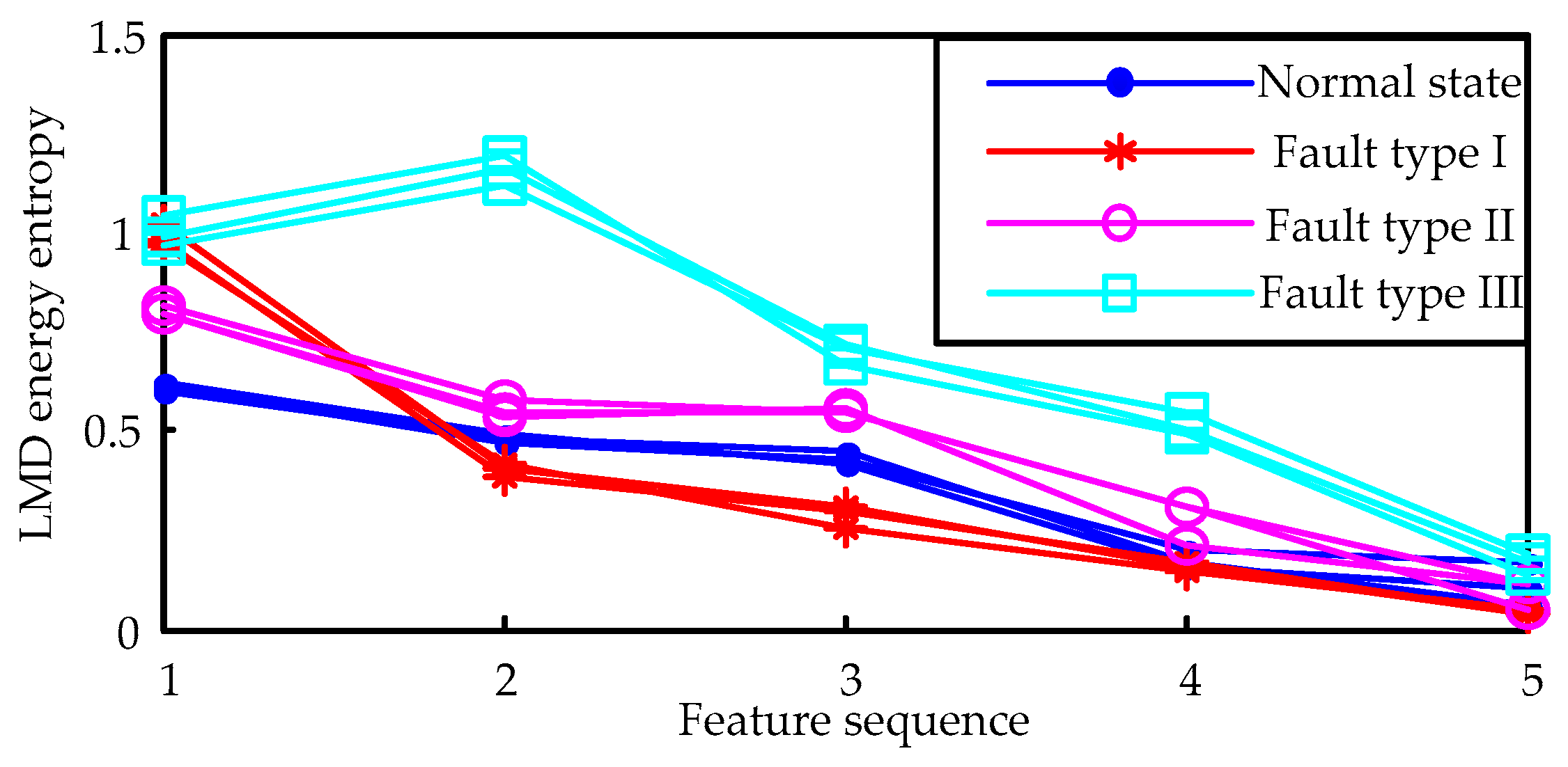
3. Feature Extraction Based on Time Segmentation Energy Entropy

By using LMD, a multi-component signal can be decomposed into a set of mono-component PF components and a residue. The PF components contain different frequency bands ranging from high to low, so the energy distribution of each PF component generally has obvious differences. However, as shown in Figure 2, although time-frequency characteristics and energy distribution of different fault types can be found through visual observation, it is difficult to recognize the HVCB fault only through simple statistic characteristics (such as maximum, minimum) due to the vibration signal with complex nonlinear structure. Entropy describes the disorder degree in a system. As an important part of information theory, Shannon entropy is effective in measuring the disorder degree of information, especially for a complicated nonlinear signal [32]. It has been widely applied to evaluation of mechanical conditions and the fault diagnosis field.

Assuming a system appears in several different states $x_1,x_2,\cdots ,x_N$, the probability of state $x_j$ is denoted by $P_j$, and the Shannon entropy $H$ of this system can be defined as:

$$H=-{\displaystyle \sum _{j=1}^N{P}_j}\log P_j,$$

(13)

where $P_j\in [0,1]$ and ${\displaystyle \sum _{j=1}^N{P}_j}=1$. When $P_j=0$, $P_j\log P_j=0$.

The energy distribution of the HVCB vibration signal changed in different frequency areas. When the mechanical faults of HVCB occur, vibration frequency of different parts of mechanical structures will be changed significantly. The energy distribution in the same frequency band of different types of vibration signals has significant differences. Therefore, each frequency component of vibration signals contains important fault information. The energy entropy [11], developed by Shannon entropy, can make a quantitative description of energy distribution in both time and frequency domains. The energy entropy of each PF component can be chosen to construct the feature vector for mechanical fault diagnosis, but it is difficult to identify the time-delay faults of HVCBs by energy entropy of each component. To improve the identification ability of time-delay faults of HVCBs, time segmentation energy entropy (TSEE) is introduced to extract feature vectors.

On the other hand, the different PF contains different characters of time-frequency energy distribution for fault diagnosis with different effects. The level of PFs used for feature extraction should be chosen first. Generally, the first few PF components contain the most important and effective fault information [10,12]. For the different energy distributions, we can compute the ratio of energy of each PF component to that of the original signal [12]. The ratio, which is called energy ratio here, is regarded as the selection criterion of PF components. To enhance the persuasion of experimental results, we take the average of energy ratio of three vibration signals per type. The energy ratio distribution of four types of vibration signals is shown in Figure 4.

From Figure 4, we find that the first five PF components of each type of signal contain most of the energy. Therefore, the first five PF components are chosen to form a component matrix first. Then, the whole component matrix is segmented into 30 equal sub-matrixes along the time axis (according to the length of time of signals and the effectiveness of extracted features). Each sub-matrix contains five time-frequency blocks. Finally, energy entropies of these sub-matrixes are extracted to compose the TSEE feature vector. The segmentation of the component matrix of the normal signal is shown in Figure 5.

Let $E_{i,j}$ be the energy contained in time-frequency block $B_{i,j}$ $(i=1,2,\cdots ,5;j=1,2,\cdots ,30)$, and $E$ the total energy contained in the whole component matrix. $E_{i,j}$ is normalized as

$$e_{i,j}=E_{i,j}/E,$$

(14)

According to the basic theory of energy entropy, TSEE of each type of signal can be calculated by:

$$H_j=-{\displaystyle \sum _{i=1}^5{e}_{i,j}\cdot \log e_{i,j}},j=1,2,\cdots ,30,$$

(15)

The feature vector of HVCB vibration signals is written as $H=[H_1,H_2,\cdots ,H_{30}]$. H is regarded as the input vector of a hybrid classifier to diagnose HVCB faults.

4. Hybrid Classifier with Support Vector Data Description (SVDD) and Fuzzy C-Means (FCM)

Due to the excessive dependence of training samples, a traditional multi-class classifier can misidentify the fault types without training samples as normal samples or the wrong type. Therefore, a hybrid classifier based on SVDD and FCM is used for fault diagnosis of HVCBs.

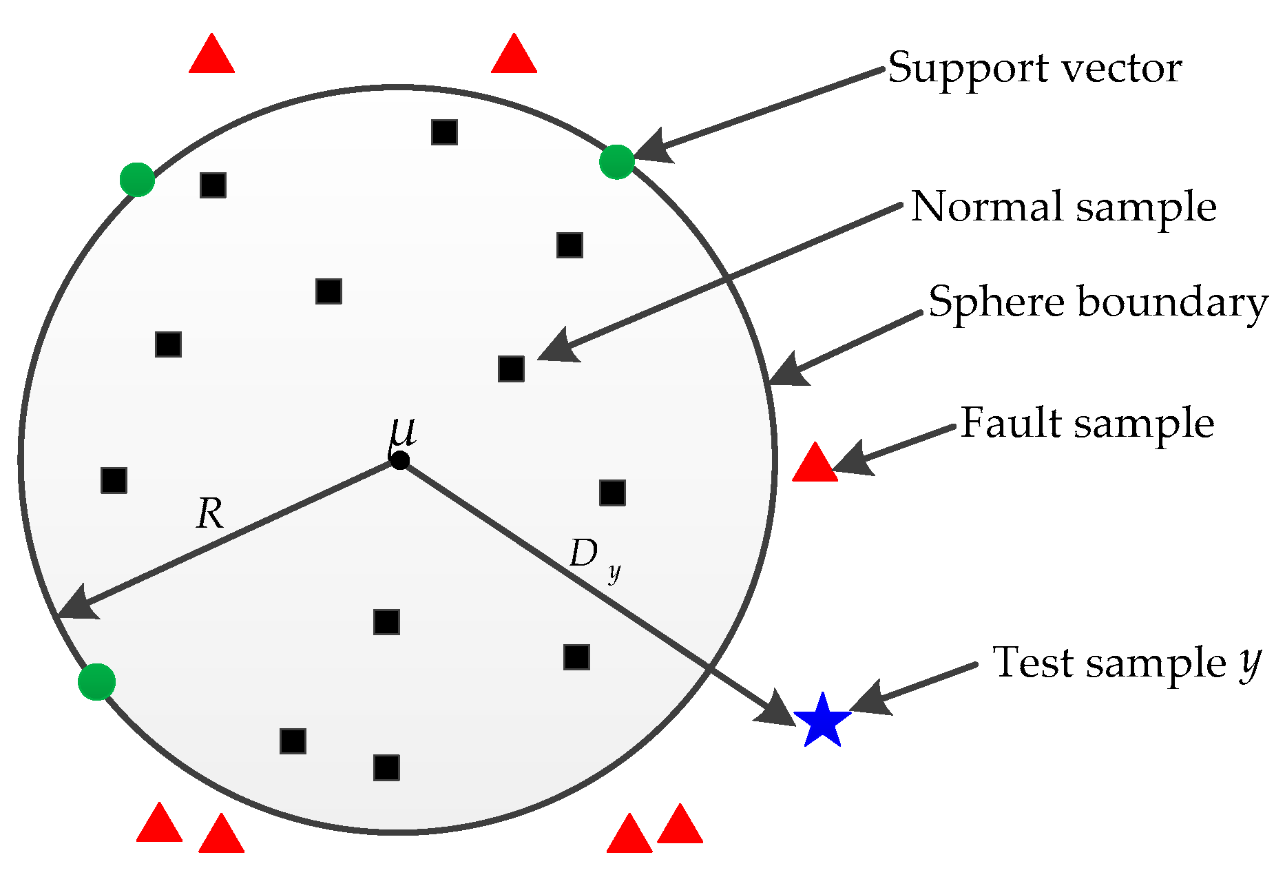
4.1. Support Vector Data Description

Support Vector Data Description (SVDD) has received widespread attention in the field of condition monitoring [33,34]. The basic idea of SVDD is to compute a spherically shaped decision boundary with minimum radius that encloses most of target samples in a high dimension feature space [33,34,35,36], as illustrated in Figure 6.

Given datasets $x_i,i=1,2,\mathrm{...},n$, they are mapped into a high-dimensional feature space through nonlinear mapping $\varphi :x\to \varphi (x)$ at first. Then a hypersphere $(\mu ,R)$ with minimum volume that encloses most of target samples is obtained in feature space, where $\mu$ and $R$ denote the center and radius of the hypersphere respectively. This may boil down to the following quadratic programming problem:

$$\{\begin{array}{l}minF(R,\mu ,\xi )=R^2+C{\displaystyle \sum _i{\xi }_i}\\ s.t.{\Vert \varphi \left(x_i\right)-\mu \Vert }^2\le R^2+{\xi }_i,{\xi }_i\ge 0,\forall i\end{array},$$

(16)

where ${\xi }_i$ is a slack variable, it is introduced to allow some sample points to lie outside the sphere. $C$ is the penalty parameter, which is used to control the tradeoff between the volume of the hypersphere and the number of outliers.

A kernel function is chosen to satisfy the condition of $K(x_i,x_j)=\langle \varphi (x_i),\varphi (x_j)\rangle$, where $\langle \varphi (x_i),\varphi (x_j)\rangle$ denotes the inner product of $\varphi (x_i)$ and $\varphi (x_j)$ in feature space. The expression of RBF Gaussian kernel function adopted in this paper is as follows:

$$K(x_i,x_j)=\exp \left\{-\frac{{\Vert x_i-x_j\Vert }^2}{2{\sigma }^2}\right\},$$

(17)

In order to solve the optimization problem (16), Lagrange multipliers ${\alpha }_i$ are introduced. Then, Equation (16) is transformed into

$$\{\begin{array}{l}\underset{{\alpha }_i}{max}L={\displaystyle \sum _i{\alpha }_{i}K(x_i,x_i)}-{\displaystyle \sum _{i,j}{\alpha }_i{\alpha }_{j}K(x_i,x_j)}\\ s.t.{\displaystyle \sum _i{\alpha }_i}=1,i=1,2,\cdots ,n\\ 0\le {\alpha }_i\le C,i=1,2,\cdots ,n\end{array},$$

(18)

Lagrange multipliers ${\alpha }_i$ can be obtained by Equation (18). When ${\alpha }_i>0$, the corresponding sample $x_s$ is called a support vector. The radius of the hypersphere can be obtained by:

$$R^2=K\left(x_s,x_s\right)-2{\displaystyle \sum _i{\alpha }_{i}K(x_i,x_s)}+{\displaystyle \sum _{i,j}{\alpha }_i{\alpha }_{j}K(x_i,x_j)},$$

(19)

After completing all of the above process, the training of SVDD is finished. Here, we choose the normal signals as target samples. Thus, for any given HVCB vibration sample $y$, the distance $D$ from the sample point to the center of the hypersphere is used to compare with the radius of the hypersphere. Then, if there are mechanical faults of HVCBs, they can be detected. The distance $D$ can be calculated by:

$$D_y^2={\Vert y-\mu \Vert }^2=K(y,y)-2{\displaystyle \sum _i{\alpha }_{i}K(x_i,y)}+{\displaystyle \sum _{i,j}{\alpha }_i{\alpha }_{j}K(x_i,x_j)},$$

(20)

If $D_y^2>R^2$, it shows that test sample $y$ is a fault sample. Otherwise, it is a normal sample. Because of the insufficient samples of HVCB faults, SVDD has the over-fitting problem to some extent. SVDD is only suitable for separating the testing set into two types. Therefore, the excessive use of SVDDs will increase the complexity and degree of over-fitting of the classifier.

4.2. Fuzzy C-Means Algorithm

The fuzzy c-means algorithm (FCM), based on objective function, is one of the most classic clustering algorithms. It is very useful for unsupervised clustering. The objective of FCM adopted in the new method is to carry on preliminary classification of the new sample which is confirmed as a fault condition. In the condition of taking the number of known fault types as the clustering number, the possible type of the new sample can be determined only by clustering analysis of one time. On this basis, only one additional SVDD classifier is needed to judge whether the new sample belongs to an unknown type or not. Therefore, the use of FCM in the new method is not only able to reduce the complexity of the classifier, but also helps avoid the over-fitting problem caused by the excessive use of SVDDs.

Let $\mathit{X}=\left\{x_1,x_2,\cdots ,x_n\right\}$ as a data set; $\mathit{Z}={[z_1,z_2,\cdots ,z_c]}^{\mathrm{T}}$ is cluster center vector; $\mathit{U}={[u_{ij}]}_{n\times c}$ is the membership matrix; c is the number of clusters; n is the number of data samples; $u_{ij}$ denotes the membership of data point $x_i$ in the $j\mathrm{th}$ cluster. The normalized $u_{ij}$ must satisfy the following condition:

$$\{\begin{array}{l}{\displaystyle \sum _{j=1}^c{u}_{ij}=1},\forall i\\ u_{ij}\in [0,1],\forall i,j\\ 0<{\displaystyle \sum _{i=1}^n{u}_{ij}<n,\forall n}\end{array},$$

(21)

${\delta }_{ij}$ is the Euclidean distance between data point $x_i$ and clustering center $z_j$, it can be calculated by the following Equation:

$${\delta }_{ij}=\Vert x_i-z_j\Vert ={(x_i-z_j)}^{\mathrm{T}}(x_i-z_j),$$

(22)

In order to get the membership matrix $\mathit{U}$, the objective function of FCM is defined as:

$$J(\mathit{U},\mathit{Z})={\displaystyle \sum _{i=1}^n{\displaystyle \sum _{j=1}^c{(u_{ij})}^t{({\delta }_{ij})}^2}},$$

(23)

where t is the weighting fuzziness parameter. It must satisfy the condition of $t>1$ to get the good result and it is generally chosen as 2. The essence of FCM clustering is an iterative process to calculate the membership matrix $\mathit{U}$ and cluster center vector $\mathit{Z}$ which minimize the objective function $J$. The steps are as follows [28]:

• FCM Algorithm
• Step 1. Determine c and t, initialize $\mathit{U}$ and let $iter=0$, ($\epsilon >0$).
• Step 2. Compute clustering centers ($z_j$) by Equation (24):

  $$z_j={\displaystyle \sum _{i=1}^n{(u_{ij})}^t{x}_i/{\displaystyle \sum _{i=1}^n{(u_{ij})}^t}},$$

  (24)
• Step 3. Update $\mathit{U}$ by Equation (25):

  $$u_{ij}=1/{\displaystyle \sum _{w=1}^c{({\delta }_{ij}/{\delta }_{wj})}^{\frac{2}{t-1}}},$$

  (25)
• Step 4. Compute $\Vert z^{(iter+1)}-z^{(iter)}\Vert$,
• IF $\Vert z^{(iter+1)}-z^{(iter)}\Vert <\epsilon$, STOP
• ELSE $iter=iter+1$, return to Step 2.

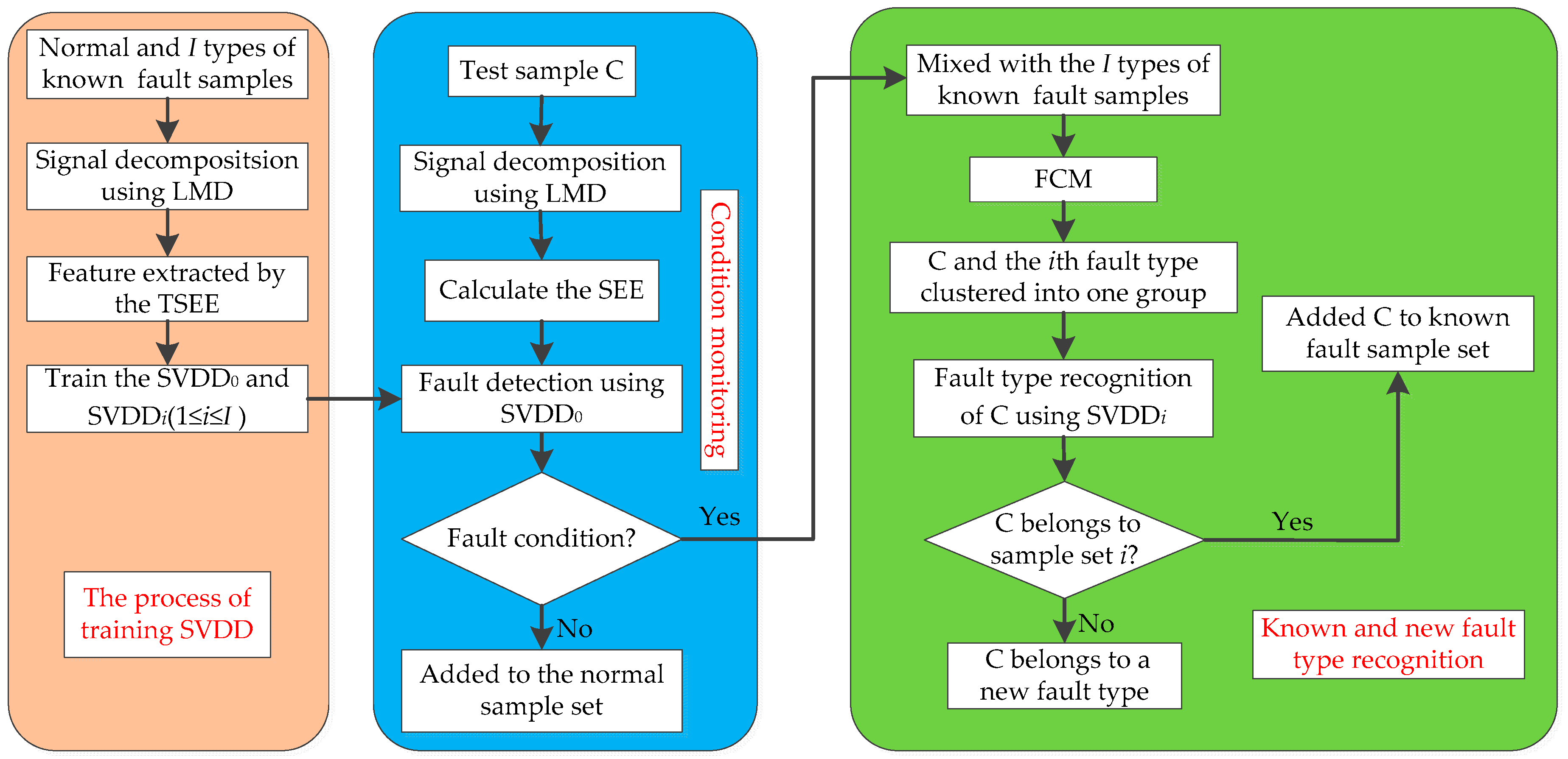
4.3. Fault Diagnosis Process of the New Method

In order to solve the problem whereby traditional analyses can easily misidentify unknown fault types as normal condition or known fault types, a novel mechanical fault diagnosis method of HVCBs based on LMD, TSEE and hybrid classifier is proposed. On the premise of feature extraction using LMD, TSEE feature is extracted by time-domain segmentation, then a hybrid classifier constructed with SVDD and FCM is used for fault diagnosis. In the process of classification, SVDD is first used to judge whether a fault occurs. If a mechanical fault is confirmed, FCM is used to carry on preliminary classification of the fault sample. According to the clustering result, corresponding SVDD can be used to judge whether the fault sample belongs to an unknown type or not.

The whole process of fault diagnosis method proposed in this paper is as follows:

(1)

LMD is used to decompose vibration signals of HVCBs into a series of PFs.

(2)

The first five PF components are chosen according to energy ratio to form a component matrix; the whole component matrix is then segmented into 30 equal time-domain sub-matrixes along the time axis. Each sub-matrix contains five time-frequency blocks. Then energy entropies of these sub-matrixes are extracted to compose the TSEE feature vector.

(3)

The normal samples are used to train the SVDD denoted as $\mathrm{SVD}{\mathrm{D}}_0$. Through $\mathrm{SVD}{\mathrm{D}}_0$, fault samples are determined. Subsequently, fault sample and I types of known fault samples are clustered using the FCM method with cluster number I, before the corresponding $\mathrm{SVD}{\mathrm{D}}_i(1\le i\le I)$ is chosen to judge whether the fault sample belongs to a new type or not. $\mathrm{SVD}{\mathrm{D}}_i$ is trained with the $i\mathrm{th}$ type of known fault samples.

Figure 7 shows the flow chart of the fault diagnosis method.

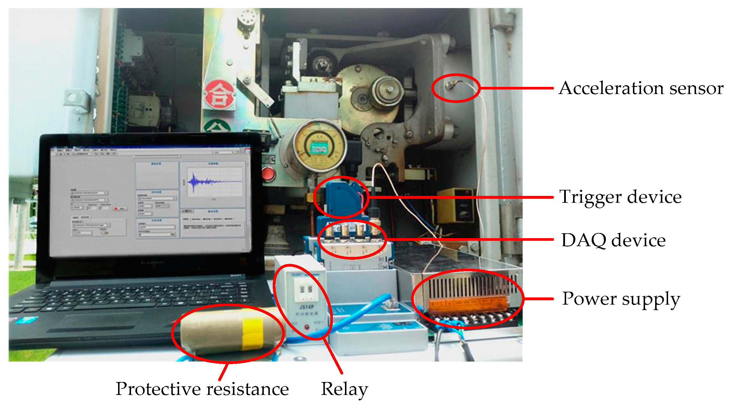
5. Experimental Results and Analysis

The experiment is carried out on a LW9-72.5 series outdoor SF₆ HVCB (Siemens High Voltage Switchgear, Shanghai, China). In the vibration signal acquisition system, a CA-YD-182A piezoelectric acceleration sensor (Jiangsu United Electronic Technology, Yangzhou, China) is used to collect the vibration signal. The NI-9234 DAQ device made by National Instruments (NI, Austin, TX, USA) is used to record the data. Figure 8 shows the vibration signal acquisition system for a HVCB. The sampling frequency is 25.6 kS/s. When HVCBs receive a related command, the vibration signal acquisition system receives the command at the same time and starts recording the vibration data. Therefore, each signal sample takes the same amount time that HVCBs need to receive the startup command to begin recording data. It is useful for analyzing time-delay faults of HVCBs. With the purpose of avoiding HVCB damage from excessive opening/closing operation, just 40 samples per fault type and 40 normal samples were collected.

5.1. Performance Comparison between LMD and Empirical Mode Decomposition (EMD)

The essence of the end effect is that the envelope of the signal is distorted, which will add some fake components to the original signal. Therefore, the total energy of components will be increased. The change of energy before and after decomposition can be used to evaluate the influence of the end effect [34].

In order to make a quantitative evaluation of decomposition results of LMD and EMD, the change of root mean square (RMS) is regarded as an index to indicate the change of energy before and after decomposition [37]. The evaluation index $\theta$ is defined as:

$$\theta =\frac{\left|({\displaystyle \sum _{m=1}^{d}RM{S}_{P{F}_m}+RM{S}_u})-RM{S}_x\right|}{RM{S}_x},$$

(26)

where $RM{S}_{P{F}_m}$, $RM{S}_u$, and $RM{S}_x$ denote the RMS of the $m\mathrm{th}$ PF component, the RMS of residue $u_d$ and the RMS of original signal $x(t)$, respectively. The RMS of original signal $x(t)$ can be obtained by:

$$RM{S}_x=\sqrt{[{\displaystyle \sum _{f=1}^T{x}^2(f)}]/T},$$

(27)

in which, $f=1,2,\cdots ,T$ denotes the number of sampling points and T = 3840.

According to the definition of $\theta$, it is nonnegative. Moreover, a higher value of $\theta$ indicates the larger change of energy, the greater influence of end effect and the lower precision.

Three normal signals were chosen as test samples, and then decomposed by LMD and EMD respectively. The average number of components, average decomposition time and evaluation index $\theta$ obtained by LMD and EMD are shown in

Table 1. The contrast of LMD and EMD decomposition result.

Decomposition Method	Average Number of Components	Average Decomposition Time/s	Average Evaluation Index θ
LMD	8	0.076	0.235
EMD	11	0.242	0.389

.

Based on Table 1, we find that the average number of components obtained by the LMD method is less than EMD. This characteristic guarantees that the feature information will not be divided into a few adjacent decomposition levels which contain similar information. It improves the efficiency and precision of the decomposition result of LMD. In terms of decomposition time, the EMD method needs more time than LMD. This is because cubic spline interpolation is used to create the upper and lower envelopes in the process of EMD. Furthermore, the value of evaluation index $\theta$ obtained by LMD is smaller than EMD, i.e., the energy of components obtained by LMD has smaller change, which may reduce the influence of end effect to some extent.

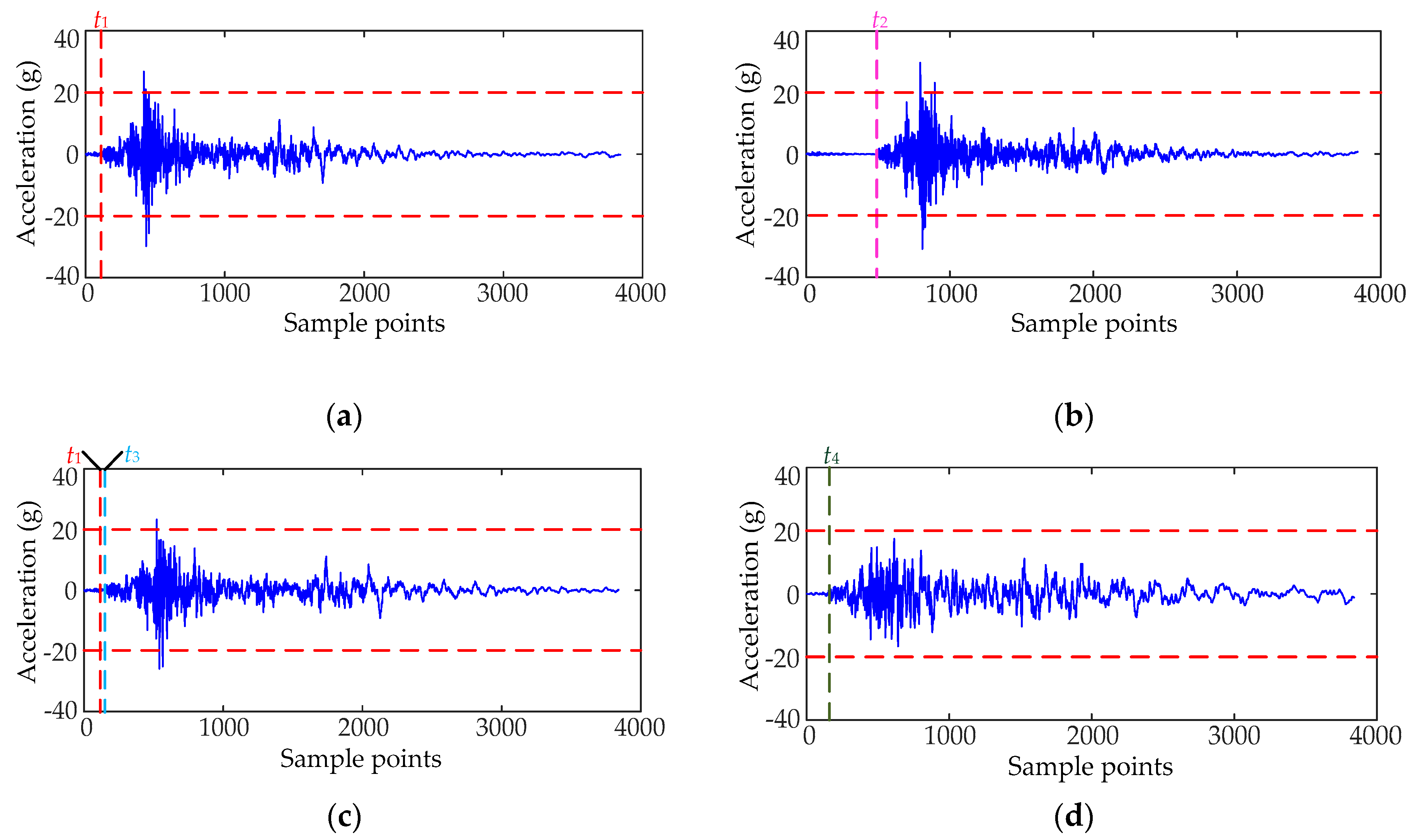
5.2. Feature Extraction of Measured Signals and Analysis

Figure 9 shows the TSEE feature distribution of four types of vibration signals. For the sake of clarity, only three data samples of each type are listed. Figure 9 shows that feature distributions of different types of vibration signals have obvious differences. The fourth characteristic value of the normal signal is the maximum. Compared with the normal signals, the occurrence moments of the maximum of TSEE extracted from fault type I and fault type II are delayed to different degrees. The maximum of TSEE extracted from the fault type III is less than the other three signals.

In the literature [9], the energy entropy of intrinsic mode function (IMF), which was called EMD energy entropy, was extracted. To validate the superiority of the feature extraction method proposed in this study, we follow the feature extraction method in the literature [9], and extracted energy entropy of five PF components to construct a five-dimension feature vector. Here the energy entropy of each PF component is called LMD energy entropy. Figure 10 shows the LMD energy entropy feature distribution of four types of vibration signals. For the sake of clarity, only three data samples of each type is listed. As is evident in Figure 10, there are no significant differences in the LMD energy entropy feature distribution of four types of signals, especially for normal signal and time-delay fault signals. This characteristic of the LMD energy entropy method will degrade the performance of a classifier. A more comprehensive comparison between TSEE and LMD energy entropy in diagnosis ability is made in the following section.

5.3. Fault Diagnosis Using Hybrid Classifier Based on SVDD and FCM

To prove the ability to distinguish normal and fault states of different classification methods, a comparison among SVDD, SVM and BPNN is presented. The TSEE is selected as the input vector of the classifier. Before using a classifier to classify new content, we first need to train the classifier. The 20 samples of each type are selected randomly as the train samples. The remaining 20 samples of each type are taken as test samples. The training samples of the normal state are used to train $\mathrm{SVD}{\mathrm{D}}_0$. A total of 60 training samples of normal state, fault type I and fault type III are used to train the SVM and BPNN. The remaining 60 samples of those three types are chosen as test samples. Constant parameters of the SVDD are set as $C=0.33$, $\sigma =0.71$ in accordance with the method in the literature [38]. The discriminant results of the types contained in the training samples are shown in

Table 2. Fault-detection ability of different classifiers with TSEE.

Classifier	Test Sample	Discriminant Result		State Discriminant Accuracy/%
		Normal State	Fault State
$\mathrm{SVD}{\mathrm{D}}_0$	Normal state	19	1	95
	Fault type I	0	20	100
	Fault type III	0	20	100
SVM	Normal state	18	2	90
	Fault type I	0	20	100
	Fault type III	3	17	85
BPNN	Normal state	18	2	90
	Fault type I	0	20	100
	Fault type III	4	16	80

, where the state discriminant accuracy is used to reflect the ability of different classifiers to judge whether there is a fault in the HVCBs.

As illustrated in Table 2, for the normal and fault-type samples with training samples, the fault-detection accuracy of SVDD is significantly higher than that of SVM and BPNN. Although SVDD failed to identify all the normal samples, it has not identified fault samples as normal samples. The classification ability of SVM approximates with BPNN methods. However, for fault type III, both of the two methods mistakenly identified some fault samples as normal samples. In fact, for HVCB fault detection, the impact of misidentifying fault samples as normal is much more serious than misidentifying normal samples as fault. Thus, for the types contained in the training samples, SVDD has better fault-detection ability than SVM and BPNN. In order to compare the detection effectiveness of the TSEE and LMD energy entropy feature, we select LMD energy entropy as input feature vector to repeat the above experiment, and a comparative result is shown in

Table 3. Fault-detection ability of different classifier with LMD energy entropy.

Classifier	Test Sample	Discriminant Results		State Discriminant Accuracy/%
		Normal State	Fault State
$\mathrm{SVD}{\mathrm{D}}_0$	Normal state	16	4	80
	Fault type I	2	18	90
	Fault type III	1	19	95
SVM	Normal state	14	6	70
	Fault type I	7	13	65
	Fault type III	2	18	90
BPNN	Normal state	15	5	75
	Fault type I	9	11	55
	Fault type III	2	18	90

.

From Table 1 and Table 3 it can be seen, when selecting the LMD energy entropy as the input feature vector, the state detection results of three classification methods are dramatically inferior to those obtained by using TSEE, especially for the normal states and time-delay faults. Therefore, LMD energy entropy is not suitable for HVCB mechanical fault detection.

Some new fault types maybe occur in the real power systems. At this point, due to a lack of training samples, traditional multi-classification methods can misidentify these fault types as normal state, which will affect the stable operation of the power system. Therefore, it is very important to identify the new fault types as unknown fault states by accurately using the classifier. A contrast experiment was designed to compare the unknown fault-detection ability of SVDD, SVM and BPNN. In this experiment, 20 samples of fault type II are chosen as test samples and not joined in training samples. The detection results of fault samples without training samples are shown in

Table 4. Detection results of the fault type (fault type II) without training samples.

Classifier	Discriminant Results		State Discriminant Accuracy/%
	Normal State	Fault State
SVDD	0	20	100
SVM	18	2	10
BPNN	19	1	5

.

As shown in Table 4, SVDD can accurately identify fault types without training samples of fault states. However, almost all of the fault types without training samples are misidentified as normal samples by SVM and BPNN. Therefore, SVDD has better ability to distinguish normal and fault states of HVCBs.

In order to prove the ability to distinguish known and unknown fault types, a comparison among the new hybrid classifier, SVM and BPNN is presented. Fault type I and fault type III are selected as the known fault type with training samples. Fault type II is selected as the unknown fault type without training samples. Twenty samples of each known fault type are randomly selected as the train samples for SVDD, SVM and BPNN. Two SVDD classifiers denoted as $\mathrm{SVD}{\mathrm{D}}_i(1\le i\le 2)$ are trained to distinguish known (fault type I and fault type III) and unknown fault types (fault type II). The remaining 40 samples of two known fault types and 20 samples of unknown fault type are selected as test samples. In the new method, the number of clusters is two and the threshold $\epsilon$ is set to $\epsilon =0.0001$; corresponding trained $\mathrm{SVD}{\mathrm{D}}_i$ is used to judge whether the fault sample belongs to a new type or the known fault type. The diagnosis result is shown in

Table 5. Fault diagnosis results comparison of different methods.

Classifier	Test	Diagnosis Results			Recognition
	Sample	Fault Type I	Fault Type III	New Type	Accuracy/%
	Fault type I	20	0	0	100
Hybrid Classifier	Fault type II	0	0	20	100
	Fault type III	0	20	0	100
	Fault type I	19	1	0	95
SVM	Fault type II	0	20	0	0
	Fault type III	2	18	0	90
	Fault type I	18	2	0	90
BPNN	Fault type II	0	20	0	0
	Fault type III	2	18	0	90

.

Table 5 shows that the new method can correctly distinguish the known fault type and unknown fault type, and its recognition accuracy of a new fault type is 100%, whereas that of SVM and BPNN is 0. It indicates the new method shows a conspicuous advantage in new-type recognition. For the known fault samples, the new method can correctly judge their fault types. Furthermore, in a real power system environment, only a vibration signal of HVCBs can be collected each time. The new method makes a judgment to only one sample each time, which is more consistent with actual demand of HVCB fault diagnosis.

6. Conclusions

A novel fault diagnosis method using a hybrid classifier based on Local Mean Decomposition (LMD) and time segmentation energy entropy (TSEE) is proposed in this paper. The main contributions of this research are as follows:

(1)

LMD is successfully used to process and analyze vibration signals of high-voltage circuit breakers (HVCBs) with great feature presentation ability and avoids the limitation of empirical mode decomposition (EMD) such as end effect, mode confusion and high time consumption.

(2)

The TSEE is extracted as the feature vectors. Compared to LMD energy entropy, it has high resolution time-frequency energy distribution character presentation ability especially, for time-delay fault diagnosis.

(3)

The hybrid classifier based on Support Vector Data Description (SVDD) and fuzzy c-means (FCM) not only detects the fault state accurately, but also determines whether fault samples belong to new fault types or not. Therefore, the new hybrid classifier can satisfy the high reliability requirements of the power system.

The comparative experimental results demonstrated the effectiveness and advancement of the presented method.

References

1. Landry, M.; Léonard, F.; Landry, C.; Beauchemin, R.; Turcotte, O.; Brikci, F. An improved vibration analysis algorithm as a diagnostic tool for detecting mechanical anomalies on power circuit breakers. IEEE Trans. Power Deliv. 2008, 23, 1986–1994. [Google Scholar] [CrossRef]
2. Meng, Y.P.; Jia, S.L.; Shi, Z.Q.; Rong, M.Z. The detection of the closing moments of a vacuum circuit breaker by vibration analysis. IEEE Trans. Power Deliv. 2006, 21, 652–658. [Google Scholar] [CrossRef]
3. Razi-Kazemi, A.A.; Vakilian, M.; Niayesh, K.; Lehtonen, M. Circuit-breaker automated failure tracking based on coil current signature. IEEE Trans. Power Deliv. 2014, 29, 283–290. [Google Scholar] [CrossRef]
4. Hussain, A.; Lee, S.J.; Choi, M.S.; Brikci, F. An expert system for acoustic diagnosis of power circuit breakers and on-load tap changers. Expert Syst. Appl. 2015, 42, 9426–9433. [Google Scholar] [CrossRef]
5. Huang, N.T.; Chen, H.J.; Zhang, S.X.; Cai, G.W.; Li, W.G.; Xu, D.G.; Fang, L.H. Mechanical faults diagnosis of high voltage circuit breakers based on wavelet time-frequency entropy and one-class support vector machine. Entropy 2016, 18, 7. [Google Scholar] [CrossRef]
6. Runde, M.; Aurud, T.; Lundgaard, L.E.; Ottesen, G.E.; Faugstad, K. Acoustic diagnosis of high voltage circuit-breakers. IEEE Trans. Power Deliv. 1992, 7, 1306–1315. [Google Scholar] [CrossRef]
7. Runde, M.; Ottesen, G.E.; Skyberg, B.; Ohlen, M. Vibration analysis for diagnostic testing of circuit-breakers. IEEE Trans. Power Deliv. 1996, 11, 1816–1823. [Google Scholar] [CrossRef]
8. Liu, R.N.; Yang, B.Y.; Wang, S.B.; Chen, X.F. Time-frequency atoms-driven support vector machine method for bearings incipient fault diagnosis. Mech. Syst. Signal Process. 2016, 75, 345–370. [Google Scholar] [CrossRef]
9. Ben, A.J.; Fnaiech, N.; Saidi, L.; Chebel-Morello, B.; Fnaiech, F. Application of empirical mode decomposition and artificial neural network for automatic bearing fault diagnosis based on vibration signals. Appl. Acoust. 2015, 89, 16–27. [Google Scholar] [CrossRef]
10. Liu, H.H.; Han, M.H. A fault diagnosis method based on local mean decomposition and multi-scale entropy for roller bearings. Mech. Mach. Theor. 2014, 75, 67–78. [Google Scholar] [CrossRef]
11. Huang, J.; Hu, X.G.; Geng, X. An intelligent fault diagnosis method of high voltage circuit breaker based on improved EMD energy entropy and multi-class support vector machine. Electr. Power Syst. Res. 2011, 81, 400–407. [Google Scholar] [CrossRef]
12. Han, M.H.; Pan, J.L. A fault diagnosis method combined with LMD, sample entropy and energy ratio for roller bearings. Measurement 2015, 76, 7–19. [Google Scholar] [CrossRef]
13. Tian, Y.; Ma, J.; Lu, C.; Wang, Z.L. Rolling bearing fault diagnosis under variable conditions using LMD-SVD and extreme learning machine. Mech. Mach. Theor. 2015, 90, 175–186. [Google Scholar] [CrossRef]
14. Huang, J.; Hu, X.G.; Yang, F. Support vector machine with genetic algorithm for machinery fault diagnosis of high voltage circuit breaker. Measurement 2011, 44, 1018–1027. [Google Scholar] [CrossRef]
15. Sanchez, H.; Escobet, T.; Puig, V. Fault diagnosis of advanced wind turbine benchmark using interval-based ARRs and observers. IEEE Trans. Ind. Electron. 2015, 62, 3783–3793. [Google Scholar] [CrossRef]
16. Yan, X.G.; Edwards, C. Nonlinear robust fault reconstruction and estimation using a sliding mode observer. Automatica 2007, 43, 1605–1614. [Google Scholar] [CrossRef]
17. Yan, X.G.; Edwards, C. Adaptive Sliding-Mode-Observer-Based fault reconstruction for nonlinear systems with parametric uncertainties. IEEE Trans. Ind. Electron. 2008, 55, 4029–4036. [Google Scholar]
18. Gao, Z.W.; Cecati, S.; Ding, S.X. A survey of fault diagnosis and fault-tolerant techniques-Part I: Fault diagnosis with model-based and signal-based approaches. IEEE Trans. Ind. Electron. 2015, 62, 3757–3767. [Google Scholar] [CrossRef]
19. Lee, D.S.; Lithgow, B.J.; Morrison, R.E. New fault diagnosis of circuit breakers. IEEE Trans. Power Deliv. 2003, 18, 454–459. [Google Scholar] [CrossRef]
20. Chen, J.L.; Li, Z.P.; Pan, J.; Chen, G.G.; Zi, Y.Y.; Yuan, J.; Chen, B.Q.; He, Z.J. Wavelet transform based on inner product in fault diagnosis of rotating machinery: A review. Mech. Syst. Signal Process. 2016, 70–71, 1–35. [Google Scholar] [CrossRef]
21. Eren, L.; Ünal, M.; Devaney, M.J. Harmonic analysis via wavelet packet decomposition using special elliptic half-band filters. IEEE Trans. Instrum. Meas. 2008, 56, 2289–2293. [Google Scholar] [CrossRef]
22. Aktaibi, A.; Rahman, M.A.; Razali, A.M. An experimental implementation of the dq-Axis wavelet packet transform hybrid technique for three-phase power transformer protection. IEEE Trans. Appl. 2014, 50, 2919–2927. [Google Scholar] [CrossRef]
23. Smith, J.S. The local mean decomposition and its application to EEG perception data. J. R. Soc. Interface 2005, 2, 434–454. [Google Scholar] [CrossRef] [PubMed]
24. Cheng, J.S.; Yang, Y. A rotating machinery fault diagnosis method based on local mean decomposition. Digit. Signal Process. 2012, 22, 356–366. [Google Scholar] [CrossRef]
25. Zhang, X.Y.; Zhou, J.Z. Multi-fault diagnosis for rolling element bearings based on ensemble empirical mode decomposition and optimized support vector machines. Mech. Syst. Signal Process. 2013, 41, 127–140. [Google Scholar] [CrossRef]
26. Ge, M.; Xu, Y.S.; Du, R.X. An intelligent online monitoring and diagnostic system for manufacturing automation. IEEE Trans. Autom. Sci. Eng. 2008, 5, 127–138. [Google Scholar]
27. Zin, A.A.M.; Saini, M.; Mustafa, M.W.; Sultan, A.R. Rahimuddin. New algorithm for detection and fault classification on parallel transmission line using DWT and BPNN based on Clarke’s transformation. Neurocomputing 2015, 168, 983–993. [Google Scholar]
28. Cao, L.H.; Yu, J.W.; Li, Y. Study on the determination method of the normal value of relative internal efficiency of the last stage group of steam turbine. Energy 2016, 98, 101–107. [Google Scholar] [CrossRef]
29. Tax, D.M.J.; Duin, R.P.W. Support vector domain description. Pattern Recognit. Lett. 1999, 20, 1191–1199. [Google Scholar] [CrossRef]
30. Ban, O.I.; Ban, A.I.; Tuse, D.A. Importance-performance analysis by fuzzy c-means algorithm. Expert Syst. Appl. 2016, 50, 9–16. [Google Scholar] [CrossRef]
31. Orhan, K.; Özge, T.; Eda, Ö. Fuzzy c-means clustering algorithm for directional data (FCM4DD). Expert Syst. Appl. 2016, 58, 76–82. [Google Scholar]
32. Shannon, C.E. A mathematical theory of communication. Bell Syst. Tech. J. 1948, 27, 379–423. [Google Scholar] [CrossRef]
33. Li, G.N.; Hu, Y.P.; Chen, H.X.; Shen, L.M.; Li, H.R.; Hu, M.; Liu, J.Y.; Sun, K.Z. An improved fault detection method for incipient centrifugal chiller faults using the PCA-R-SVDD algorithm. Energy Build. 2016, 116, 104–113. [Google Scholar] [CrossRef]
34. Huang, J.; Yan, X.F. Related and independent variable fault detection based on KPCA and SVDD. J. Process Control. 2016, 39, 88–99. [Google Scholar] [CrossRef]
35. Du, W.L.; Tian, Y.; Qian, F. Monitoring for nonlinear multiple modes process based on LL-SVDD-MRDA. IEEE Trans. Autom. Sci. Eng. 2014, 11, 1133–1148. [Google Scholar] [CrossRef]
36. Lazzaretti, A.E.; Tax, D.M.J.; Neto, H.V.; Ferreira, V.H. Novelty detection and multi-class classification in power distribution voltage waveforms. Expert Syst. Appl. 2016, 45, 322–330. [Google Scholar] [CrossRef]
37. Ren, D.Q.; Yang, S.X.; Wu, Z.T.; Yan, G.B. Evaluation of the EMD end effect and a window based method to improve EMD. In Proceedings of the Chinese Mechanical Engineering Society Annual Meeting and the First Annual Conference of the Chinese Academy of Engineering Machinery and Vehicle Engineering Department, Hangzhou, China, 6–7 November 2006; pp. 1568–1572.
38. Fu, W.L.; Zhou, J.Z.; Li, C.S.; Xiao, H.; Xiao, J.; Zhu, W.L. Vibrate fault diagnosis for hydro-electric generating unit based on support vector data description improved with fuzzy K nearest neighbor. Proc. CSEE 2014, 34, 5788–5795. [Google Scholar]
Figure 1. The measured vibration signal waveform. (a) The signal of normal state; (b) The signal of fault type I; (c) The signal of fault type II; (d) The signal of fault type III.
Entropy 18 00322 g001
Figure 2. PFs obtained by LMD of different types of vibration signals. (a) PFs obtained by LMD under the normal state; (b) PFs obtained by LMD under the state of fault type I; (c) PFs obtained by LMD under the state of fault type II; (d) PFs obtained by LMD under the state of fault type III.
Entropy 18 00322 g002
Figure 3. IMFs obtained by EMD of different types of vibration signals. (a) IMFs obtained by EMD under the normal state; (b) IMFs obtained by EMD under the state of fault type I; (c) IMFs obtained by EMD under the state of fault type II; (d) IMFs obtained by EMD under the state of fault type III.
Entropy 18 00322 g003
Figure 4. (a) The energy ratio distribution of PFs under the normal state; (b) The energy ratio distribution of PFs under the state of fault type I; (c) The energy ratio distribution of PFs under the state of fault type II; (d) The energy ratio distribution of PFs under the state of fault type III.
Entropy 18 00322 g004
Figure 5. The segmentation of component matrix of normal signal.
Entropy 18 00322 g005
Figure 6. The basic idea of SVDD for mechanical fault detection of HVCBs.
Entropy 18 00322 g006
Figure 7. The flow chart of the fault-detection method.
Entropy 18 00322 g007
Figure 8. The vibration signal acquisition system for a circuit break.
Entropy 18 00322 g008
Figure 9. (a) TSEE feature distribution of normal state; (b) TSEE feature distribution of fault type I; (c) TSEE feature distribution of fault type II; (d) TSEE feature distribution of fault type III.
Entropy 18 00322 g009
Figure 10. LMD energy entropy feature distribution of the four types of vibration signal.
Entropy 18 00322 g010