Perturbative Treatment of the Non-Linear q-Schrödinger and q-Klein–Gordon Equations

Abstract

Interesting non-linear generalization of both Schrödinger’s and Klein–Gordon’s equations have been recently advanced by Tsallis, Rego-Monteiro and Tsallis (NRT) in Nobre et al. (Phys. Rev. Lett. 2011, 106, 140601). There is much current activity going on in this area. The non-linearity is governed by a real parameter q. Empiric hints suggest that the ensuing non-linear q-Schrödinger and q-Klein–Gordon equations are a natural manifestations of very high energy phenomena, as verified by LHC-experiments. This happens for $q-$values close to unity (Plastino et al. (Nucl. Phys. A 2016, 955, 16–26, Nucl. Phys. A 2016, 948, 19–27)). It might thus be difficult for q-values close to unity to ascertain whether one is dealing with solutions to the ordinary Schrödinger equation (whose free particle solutions are exponentials and for which $q=1$) or with its NRT non-linear q-generalizations, whose free particle solutions are q-exponentials. In this work, we provide a careful analysis of the $q\sim 1$ instance via a perturbative analysis of the NRT equations.

1. Introduction

Empirical data indicate that power-law behavior in the observed probability distribution of interesting quantities is quite frequent in the natural world [1]. It was shown in [2] that one reason for this phenomenon is detector-normalization. In most measurement devices, one finds a pre-processing step that impedes the device from being overwhelmed by data of too large an amplitude that might damage the hardware. One then appeals to statistical normalizations of input data. The data are first centered by subtraction of the estimated mean and then scaled with the estimated standard deviation. It is shown in [2] that the concomitant proceedings transform Gaussian input data into q-Gaussian output ones. We remind that a q-exponential is defined as:

$$e_q(x)={[1+(1-q)x]}^{\frac{1}{1-q}};(e_{q=1}(x)=expx).$$

(1)

In view of the above empirical considerations, it becomes clear that in the immediate neighborhood of $q=1$, it is very difficult to ascertain whether one is dealing with exponentials or q-exponentials. The first instance corresponds to free-particle solutions of the celebrated Schrödinger equation, while the second instance corresponds to free particle solutions to its q-non-linear generalizations advanced in [3,4] (see also [5,6,7]), the so called NRT equation. If we confront a particle flow, which of the two equations is governing it, the linear or the non-linear one?

In order to help find an adequate answer, we carefully study here perturbative NRT solutions in a $q\sim 1$ scenario. We hope that our considerations will shed some light on these matters.

Motivation

The motivation of this paper resides in the probability that both the q-Schrödinger equation and the q-Klein–Gordon equation might be natural manifestations of very high energy phenomena [8,9], as verified by LHC-experiments [10], for which q is close to unity. In such a case, the two equations mentioned above approach the customary Schrödinger and Klein–Gordon equations, becoming identical to them in the limit $q\to 1$. The q-Schrödinger equation we will be concerned with is [3]:

$$i\hslash \frac{\partial }{\partial t}{\left[\frac{\psi (\overrightarrow{x},t)}{\psi (0,0)}\right]}^q+\frac{{\hslash }^2}{2m}▵\left[\frac{\psi (\overrightarrow{x},t)}{\psi (0,0)}\right]=0,$$

(2)

and for q close to unity, we are allowed to write:

$${\left[\frac{\psi (\overrightarrow{x},t)}{\psi (0,0)}\right]}^q=\frac{\psi (\overrightarrow{x},t)}{\psi (0,0)}+(q-1)\frac{\psi (\overrightarrow{x},t)}{\psi (0,0)}ln\left[\frac{\psi (\overrightarrow{x},t)}{\psi (0,0)}\right].$$

(3)

The second term on the right side of Equation (3) is negligible, so that one writes:

$$i\hslash \frac{\partial }{\partial t}\left[\frac{\psi (\overrightarrow{x},t)}{\psi (0,0)}\right]+\frac{{\hslash }^2}{2m}▵\left[\frac{\psi (\overrightarrow{x},t)}{\psi (0,0)}\right]=0,$$

(4)

or:

$$i\hslash \frac{\partial }{\partial t}\psi (\overrightarrow{x},t)+\frac{{\hslash }^2}{2m}▵\psi (\overrightarrow{x},t)=0,$$

(5)

the linear, conventional de Schrödinger equation.

An analogous situation arises for the q-Klein–Gordon equation. We have:

$$\square \left[\frac{\varphi (\overrightarrow{x},t)}{\varphi (0,0)}\right]+\frac{q{m}^2{c}^2}{{\hslash }^2}{\left[\frac{\varphi (\overrightarrow{x},t)}{\varphi (0,0)}\right]}^{2q-1}=0.$$

(6)

For q close to unity, one has:

$${\left[\frac{\varphi (\overrightarrow{x},t)}{\varphi (0,0)}\right]}^{2q-1}=\frac{\varphi (\overrightarrow{x},t)}{\varphi (0,0)}+2(q-1)\frac{\varphi (\overrightarrow{x},t)}{\varphi (0,0)}ln\left[\frac{\varphi (\overrightarrow{x},t)}{\varphi (0,0)}\right].$$

(7)

Once more, the second term on the right is negligible. As a consequence, we can write:

$$\square \left[\frac{\varphi (\overrightarrow{x},t)}{\varphi (0,0)}\right]+\frac{q{m}^2{c}^2}{{\hslash }^2}\left[\frac{\varphi (\overrightarrow{x},t)}{\varphi (0,0)}\right]=0,$$

(8)

or:

$$\square \varphi (\overrightarrow{x},t)+\frac{q{m}^2{c}^2}{{\hslash }^2}\varphi (\overrightarrow{x},t)=0,$$

(9)

and then, since q is close to unity

$$\square \varphi (\overrightarrow{x},t)+\frac{m^2{c}^2}{{\hslash }^2}\varphi (\overrightarrow{x},t)=0.$$

(10)

We see then that it is very important to obtain approximate q-solutions for the two above scenarios, since these are two instances that correspond to intermediate energies [3].

2. First Order Expansion of the q Exponential as a Solution of the Non-Linear NRT q-Schrödinger Equation

As a first task, we will prove that the first order Taylor expansion, around $q=1$, of q-exponential function $e_q$, is a solution of to the non-linear q-Schrödinger equation advanced in [4]:

$$i\hslash \frac{\partial }{\partial t}{\left[\frac{\psi (x,t)}{\psi (0,0)}\right]}^q=H_0\left[\frac{\psi (x,t)}{\psi (0,0)}\right]$$

(11)

$\psi (0,0)$ a fixed wave function, where:

$$H_0=\frac{p^2}{2m}=\frac{-{\hslash }^2}{2m}{\mathsf{\nabla }}^2$$

(12)

In our case: $\psi \sim e_q$, defined as:

$$e_q={[1+\frac{i}{\hslash }(1-q)(px-Et)]}^{\frac{1}{1-q}}$$

(13)

Calling $z=\frac{i}{\hslash }(px-Et)$, we deal with:

$$e_q={\left[1+(1-q)z\right]}^{\frac{1}{1-q}}$$

(14)

The function $e_q$ tends to the usual exponential when: $q\to 1$

$$e_q{(z)|}_{q\to 1}=e^z$$

(15)

We observe that $\psi (0,0)=1$. Thus, Equation (11) reduces to:

$$i\hslash \frac{\partial {\psi }^q}{\partial t}=H_0\psi (x,t).$$

(16)

2.1. First Order Expansion of $\psi =e_q$

We obtain, after a somewhat lengthy manipulation (see Appendix A):

$$\psi \simeq e^z+(q-1)\frac{z^2}{2}{e}^z,$$

or:

$$\psi \simeq e^z\left[1+(q-1)\frac{z^2}{2}\right].$$

(17)

Note that the last relation differs from the pure exponential, for q close to unity, just by the term $(q-1)z^2/2$ above.

Moreover, we have:

$$\psi \simeq e^{\frac{i}{\hslash }(px-Et)}\left[1+(1-q)\frac{{(px-Et)}^2}{2{\hslash }^2}\right]$$

(18)

We need now the expansion for the second derivative of $e_q$ with respect to x. This involves again some extensive manipulation (see Appendix A), and one finds:

$$\frac{{\partial }^2\psi }{\partial x^2}=-\frac{p^2}{{\hslash }^2}{e}^{\frac{i}{\hslash }(px-Et)}\left[q+\frac{2i}{\hslash }(q-1)(px-Et)-\frac{(q-1)}{2{\hslash }^2}{(px-Et)}^2\right].$$

(19)

Obviously, one also needs the first order expansion of ${\psi }^q$. This expansion is in the variable q, around $q=1$, and has no obvious quantum mechanics counterpart. One writes:

$${\psi }^q=e^{qln\psi }.$$

Thus,

$$\frac{\partial {\psi }^q}{\partial q}=\frac{\partial (qln\psi )}{\partial q}{\psi }^q=\left(ln\psi +\frac{q}{\psi }\frac{\partial \psi }{\partial q}\right){\psi }^q={\psi }^{q}ln\psi +q{\psi }^{q-1}\frac{\partial \psi }{\partial q}.$$

(20)

For q=1, we obtain:

$${\left.\frac{\partial {\psi }^q}{\partial q}\right|}_{q=1}={\left.\psi \right|}_{q=1}{\left.(ln\psi )\right|}_{q=1}+{\left.\frac{\partial \psi }{\partial q}\right|}_{q=1}.$$

Since we know that:

• ${\left.\psi \right|}_{q=1}=e^z$
• ${\left.(ln\psi )\right|}_{q=1}=z$
• ${\left.\frac{\partial \psi }{\partial q}\right|}_{q=1}=\frac{z^2}{2}{e}^z,$

then,

$${\left.\frac{\partial {\psi }^q}{\partial q}\right|}_{q=1}=z{e}^z+\frac{z^2}{2}{e}^z,$$

(21)

$${\left.\frac{\partial {\psi }^q}{\partial q}\right|}_{q=1}=\frac{i}{\hslash }(px-Et)e^{\frac{i}{\hslash }(px-Et)}-\frac{{(px-Et)}^2}{2{\hslash }^2}{e}^{\frac{i}{\hslash }(px-Et)}.$$

(22)

The first order expansion of ${\psi }^q$ is then, up to a normalization constant:

$${\psi }^q\simeq {\left.{\psi }^q\right|}_{q=1}+(q-1){\left.\frac{\partial {\psi }^q}{\partial q}\right|}_{q=1}.$$

Replacing here Equations (15) and (22), we have:

$${\psi }^q\simeq e^{\frac{i}{\hslash }(px-Et)}+(q-1)\left[\frac{i}{\hslash }(px-Et)e^{\frac{i}{\hslash }(px-Et)}-\frac{{(px-Et)}^2}{2{\hslash }^2}{e}^{\frac{i}{\hslash }(px-Et)}\right].$$

(23)

Finally, we require the time derivative. The first order time derivative of ${\psi }^q$ is:

$$\frac{\partial {\psi }^q}{\partial t}=\frac{-iE}{\hslash }{e}^{\frac{i}{\hslash }(px-Et)}+(q-1)\left[\frac{-iE}{\hslash }{e}^{\frac{i}{\hslash }(px-Et)}+\frac{2E}{{\hslash }^2}(px-Et)e^{\frac{i}{\hslash }(px-Et)}\right.$$

$$\left.+\frac{iE}{2{\hslash }^3}{(px-Et)}^2{e}^{\frac{i}{\hslash }(px-Et)}\right],$$

or:

$$\frac{\partial {\psi }^q}{\partial t}=\frac{-iE}{\hslash }{e}^{\frac{i}{\hslash }(px-Et)}\left[q+\frac{2i(q-1)}{\hslash }(px-Et)-\frac{(q-1)}{2{\hslash }^2}{(px-Et)}^2\right].$$

(24)

2.2. Solution to the Non-Linear q-Schrödinger Equation

Replacing Equations (19) and (24) in the non-linear q-Schrödinger Equation (16), we find that the first order Taylor’s expansion of a q-exponential is indeed a solution of this equation with the usual eigenvalue corresponding to the free particle, $E=p^2/2m$. We have thus achieved what one might call ‘self-consistency’, indicating that our calculations have been performed correctly.

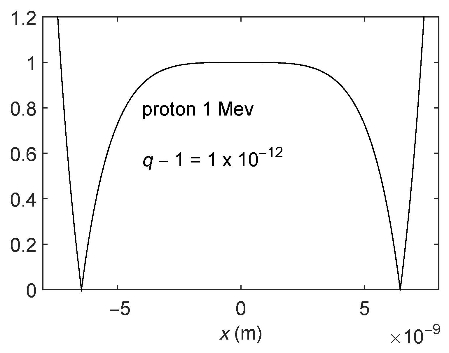
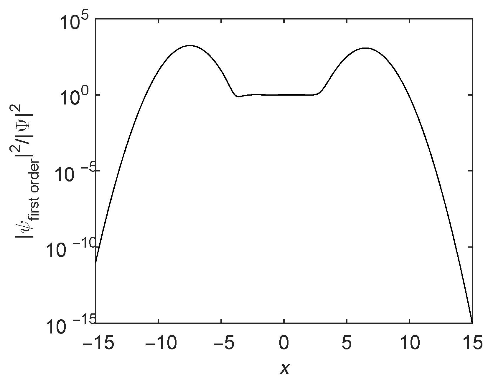
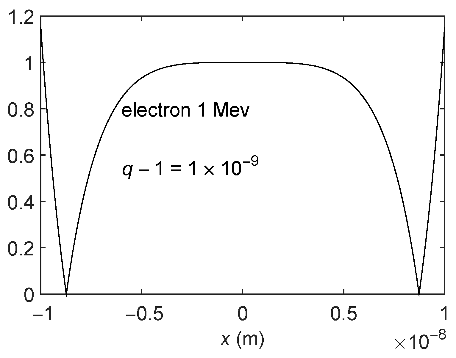
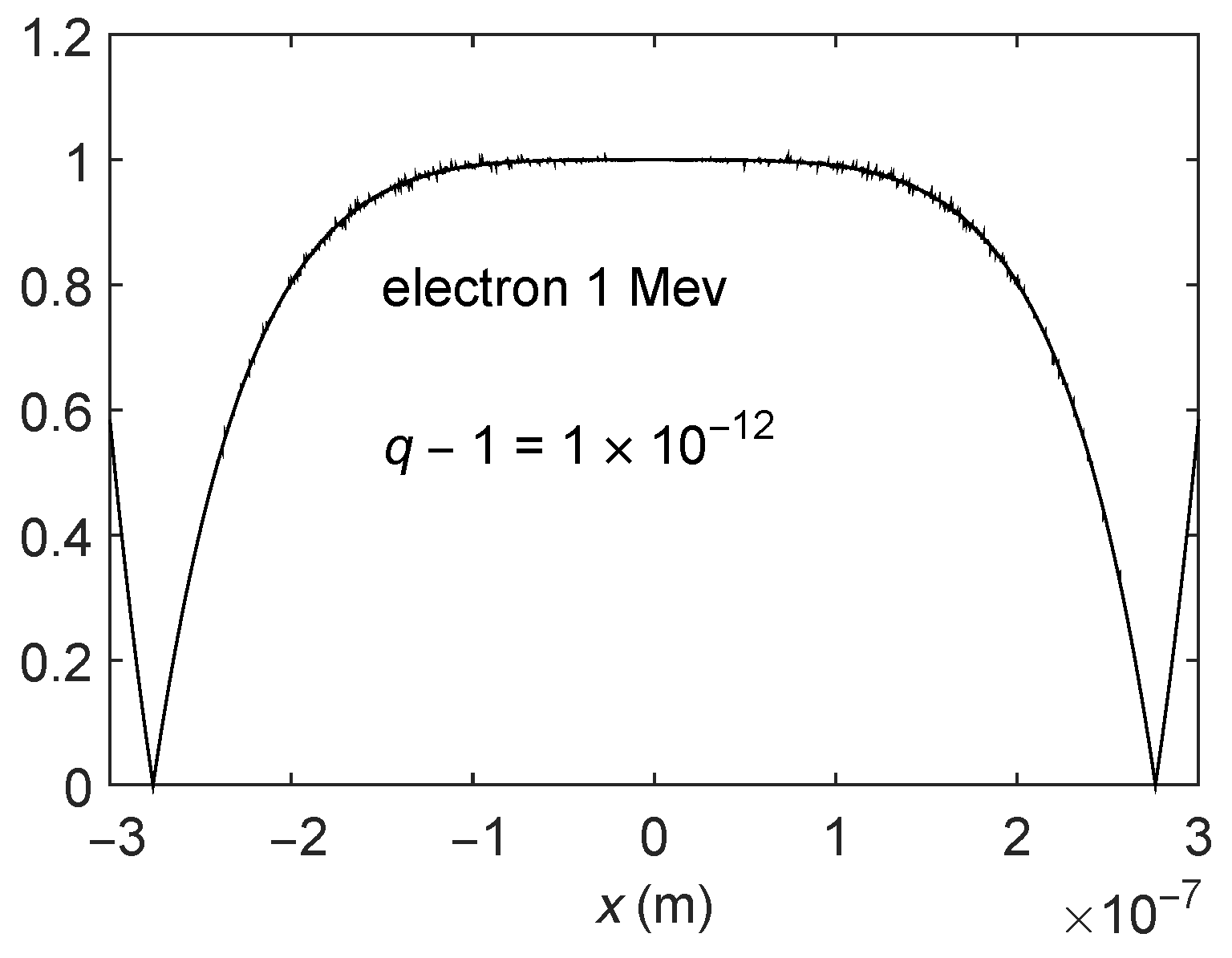
2.3. Comparison between the Exact and Approximate Solutions

In this subsection, we intend to make comparisons between the approximate and exact solutions of q-Schrödinger equation. To this end, we first try to evaluate the modulus of the ratio R of the functions (13) and (18). As an example, we display R in four figures corresponding to an electron and a proton with 1 MeV of energy at $t=0$ (Figure 1, Figure 2, Figure 3 and Figure 4). Note that, for a range of x very large in terms of atomic or nuclear relevant distances, the ratio R is essentially unity. Our approximation can then be deemed very good for the x-ranges shown in the figures, where R is close to one.

3. First Order Treatment of a q-Gaussian

From [11], selecting $mq\alpha =1$ in order to simplify the calculations, we have for the q-Gaussian:

$$\psi (x,t)={\left\{1+(q-1)\left[a(t)x^2+b(t)x+c(t)\right]\right\}}^{\frac{1}{1-q}}$$

(25)

where:

$$a(t)=\frac{mq}{1+i\hslash (q+1)t}$$

(26)

$$b(t)=\frac{1}{\beta [1+i\hslash (q+1)t]}$$

(27)

$$c(t)=\left(\frac{1}{q-1}-\frac{1}{4mq{\beta }^2}\right){\left[1+i\hslash (q+1)t\right]}^{\frac{q-1}{q+1}}+$$

$$\frac{1}{4mq{\beta }^2[1+i\hslash (q+1)t]}+\frac{1}{1-q}$$

(28)

Writing up to first order:

$$a(t)=a_1(t)+(q-1)a_2(t)$$

$$b(t)=b_1(t)+(q-1)b_2(t)$$

$$c(t)=c_1(t)+(q-1)c_2(t)$$

(29)

we obtain from Equations (26)–(28):

$$a_1(t)=\frac{m}{1+2i\hslash t}$$

(30)

$$a_2(t)=\frac{m(1+i\hslash t)}{{(1+2i\hslash t)}^2}$$

(31)

$$b_1(t)=\frac{1}{\beta (1+2i\hslash t)}$$

(32)

$$b_2(t)=-\frac{i\hslash t}{\beta {(1+2i\hslash t)}^2}$$

(33)

$$c_1(t)=\frac{1}{2}ln(1+2i\hslash t)-\frac{i\hslash t}{2m{\beta }^2(1+2i\hslash t)}$$

(34)

$$c_2(t)=\frac{1}{4m{\beta }^2}+\frac{i\hslash t}{2(1+2i\hslash t)}-\frac{(1+3i\hslash t)}{4m{\beta }^2{(1+2i\hslash t)}^2}+$$

$$\frac{1}{8}{ln}^2(1+2i\hslash t)-\frac{1+2m{\beta }^2}{8m{\beta }^2}ln(1+2i\hslash t)$$

(35)

The first order approximation for the q-Gaussian is now:

$$\psi (x,t)=\left\{1-(q-1)\left\{a_2(t)x^2+b_2(t)x+c_2(t)-\frac{1}{2}{\left[a_1(t)x^2+b_1(t)x{c}_1(t)\right]}^2\right\}\right\}\otimes$$

$$e^{-[a_1(t)x^2+b_1(t)x+c_1(t)]}$$

(36)

By construction, $\psi (x,t)$, as given by Equation (35), is a first order solution to Equation (11). Figure 5 displays the ratio between Equation (11) and (35) versus distance x (in absolute units) for $1-q={10}^{-3}$. Note that the ratio is essentially unity for distances very much larger than atomic or nuclear ones. Thus, the approximation can be considered quite good.

Comparison between the Exact and Approximate Solutions

To have an idea about the quality of the comparison between the first order treatment of the q-Gaussian and the exact solution, we evaluate the modulus of the ratio of Equations (25) and (36) in a semi-logarithmic scale. This is given in Figure 5.

4. Non-Linear q-Klein–Gordon Equation

We now wish to verify that the development of $e_q$ is a solution of the following equation:

$$\frac{1}{c^2}\frac{{\partial }^{2}F}{\partial t^2}-\frac{{\partial }^{2}F}{\partial x^2}+\frac{q{m}^2{c}^2}{{\hslash }^2}{F}^{2q-1}=0$$

(37)

This equation was advanced in [4] and re-obtained in [9].

In our case, $F=e_q$, which, let us remind the reader, is defined as:

$$e_q={[1+i(1-q)(kx-\omega t)]}^{\frac{1}{1-q}}$$

(38)

By analogy with Equations (18) and (19), we write the expansions of $e_q$ and its derivative with respect to x, respectively, as follows:

$$F\simeq e^{i(kx-\omega t)}\left[1+(1-q)\frac{{(kx-\omega t)}^2}{2}\right],$$

(39)

$$\frac{{\partial }^{2}F}{\partial x^2}=-k^2{e}^{i(kx-\omega t)}\left[q+2i(q-1)(kx-\omega t)-\frac{(q-1)}{2}{(kx-\omega t)}^2\right].$$

(40)

We should now calculate the second derivative with respect to t and the first order expansion of $q{F}^{2q-1}$, and so on. This is done in Appendix B.

Solution to the Klein–Gordon Equation

Replacing Equations (B2), (B8) and (40) in Equation (37), we find that the first order Taylor’s expansion of the q-exponential is a solution of this last equation.

5. Conclusions

We have exhaustively analyzed a first order perturbation-treatment (in q) of both the non-linear q-Schrödinger and q-Klein Gordon partial differential equations. We have shown that, for small values of $q-1$, the approximation is quite good. This is of physical significance because, as discussed in [8,9], these q values seem to be the relevant ones in the range of energies of interest for intermediate and high energy physics.

References

1. Boccara, N. Modeling Complex Systems; Springer: Berlin, Germany, 2004. [Google Scholar]
2. Vignat, C.; Plastino, A. Why is the detection of q-Gaussian behavior such a common occurrence? Physica A 2009, 388, 601–608. [Google Scholar] [CrossRef]
3. Plastino, A.; Rocca, M.C. From the hypergeometric differential equation to a non-linear Schroedinger one. Phys. Lett. A 2015, 379, 2690. [Google Scholar] [CrossRef]
4. Nobre, F.D.; Rego-Monteiro, M.A.; Tsallis, C. Nonlinear generalizations of relativistic and quantum equations with a common type of solution. Phys. Rev. Lett. 2011, 106, 140601. [Google Scholar] [CrossRef] [PubMed]
5. Plastino, A.R.; Souza, A.M.C.; Nobre, F.D.; Tsallis, C. Stationary and uniformly accelerated states in non-linear quantum mechanics. Phys. Rev. A 2014, 90, 062134. [Google Scholar] [CrossRef]
6. Plastino, A.R.; Tsallis, C. Nonlinear Schroedinger equation in the presence of uniform acceleration. J. Math. Phys. 2013, 54, 041505. [Google Scholar] [CrossRef]
7. Bountis, T.; Nobre, F.D. Travelling-wave and separated variable solutions of a nonlinear Schroedinger equation. J. Math. Phys. 2016, 57, 082106. [Google Scholar] [CrossRef]
8. Plastino, A.; Rocca, M.C. q-Gamow States as continuous linear functionals on analytical test functions. Nucl. Phys. A 2016, 948, 19–27. [Google Scholar] [CrossRef]
9. Plastino, A.; Rocca, M.C.; Ferri, G.L.; Zamora, D.J. q-Gamow States for intermediate energies. Nuc. Phys. A 2016, 955, 16–26. [Google Scholar] [CrossRef]
10. Tsallis, C. Introduction to Nonextensive Statistical Mechanics; Springer: Berlin, Germany, 2009. [Google Scholar]
11. Plastino, A.; Rocca, M.C. Hypergeometric connotations of quantum equations. Physica A 2016, 450, 435–443. [Google Scholar] [CrossRef]
Figure 1. Ratio R vs. x (in meters) for 1-MeV electrons and q 1 = 10 9 .
Entropy 19 00021 g001
Figure 2. Ratio R vs. x (in meters) for 1-MeV electrons and q 1 = 10 12 .
Entropy 19 00021 g002
Figure 3. Ratio R vs. x (in meters) for 1-MeV protons and q 1 = 10 9 .
Entropy 19 00021 g003
Figure 4. Ratio R vs. x (in meters) for 1-MeV protons and q 1 = 10 12 .
Entropy 19 00021 g004
Figure 5. q-Gaussian ratio of Equation (36) over Equation (37) vs. x (in absolute units) for q 1 = 10 3 .
Entropy 19 00021 g005