Active and Purely Dissipative Nambu Systems in General Thermostatistical Settings Described by Nonlinear Partial Differential Equations Involving Generalized Entropy Measures

Abstract

In physics, several attempts have been made to apply the concepts and tools of physics to the life sciences. In this context, a thermostatistic framework for active Nambu systems is proposed. The so-called free energy Fokker–Planck equation approach is used to describe stochastic aspects of active Nambu systems. Different thermostatistic settings are considered that are characterized by appropriately-defined entropy measures, such as the Boltzmann–Gibbs–Shannon entropy and the Tsallis entropy. In general, the free energy Fokker–Planck equations associated with these generalized entropy measures correspond to nonlinear partial differential equations. Irrespective of the entropy-related nonlinearities occurring in these nonlinear partial differential equations, it is shown that semi-analytical solutions for the stationary probability densities of the active Nambu systems can be obtained provided that the pumping mechanisms of the active systems assume the so-called canonical-dissipative form and depend explicitly only on Nambu invariants. Applications are presented both for purely-dissipative and for active systems illustrating that the proposed framework includes as a special case stochastic equilibrium systems.

1. Introduction

In a seminal work, Nambu generalized classical Hamiltonian mechanics to what is nowadays known as Nambu mechanics [1]. Nambu mechanics describes n-dimensional dynamical systems that exhibit $n-1$ invariants (i.e., integrals of motion). Applications of Nambu mechanics can be found in various fields of physics (classical mechanics, astrophysics, electrodynamics, solid state physics, hydrodynamics, nonlinear physics) and even in disciplines beyond physics.

As far as classical mechanics is concerned, a rigid body (e.g., a spinning top) rotating round and round can be considered as a system satisfying Nambu mechanics [1,2,3,4,5,6,7]. A variety of oscillatory systems [8,9,10,11,12,13,14] have been studied within the framework of Nambu mechanics. Particles moving on curved surfaces correspond under appropriate conditions to system that live in n-dimensional spaces and satisfy $n-1$ invariants, such that Nambu mechanics applies [15,16,17,18,19]. Interestingly, in astrophysics, the Kepler problem can be addressed as a special case of Nambu mechanics due to the existence of the so-called Lenz–Pauli vector, which represents a vector-valued invariant [13].

In electrodynamics, Nambu mechanics has found several applications [5,11,12,20,21]. In particular, the motion of a charged particle in a constant magnetic field can be studied from the perspective of Nambu mechanics [22]. In solid state physics, the Calogero–Moser system has been studied from the perspective of Nambu mechanics [23,24]. Moreover, Nambu mechanics has been used to calculate energy levels by means of a particular perturbation theoretical method [5]. Nambu mechanics has been used to address certain hydrodynamic problems [25,26]. In nonlinear physics, the Lorenz system has turned out to be an interesting model for applications of Nambu mechanics. Typically, a modified version of the Lorenz system that is known to be integrable is studied rather than the original chaotic system [11,27,28,29]. Furthermore, it has been shown that Nambu mechanics provides a theoretical framework to examine the dynamics of chiral models [16].

Beyond physics, it has been suggested that Nambu mechanics may be used to describe biochemical reaction equations [30,31].

Only recently, Nambu mechanics has been used to address active systems, such as limit cycle oscillators [19,28,29,32,33,34]. The notion of an active system is closely related to pumping and negative friction [35,36]. Pumping and negative friction are dissipative components. Systems exhibiting such dissipative components are likely to be affected by fluctuating forces [37]. Therefore, at issue is to discuss active Nambu systems in the context of stochastic processes. A first step in this direction has been conducted within the framework of Boltzmann–Gibbs–Shannon thermostatistics and Fokker–Planck equations that are linear with respect to their probability densities [7].

In the following sections, a more comprehensive picture of stochastic, active Nambu systems will be developed. First, general entropy measures will be considered rather than the special case of the Boltzmann–Gibbs–Shannon entropy. This will lead to Fokker–Planck equations that are nonlinear with respect to their probability densities. From a mathematical perspective, these nonlinear Fokker–Planck equations correspond to nonlinear partial differential equations. Second, non-equilibrium thermodynamic state variables will be defined that are consistent with the aforementioned generalized entropy measures. The thermodynamic state variables can be used to characterize the stochastic, active Nambu systems. Furthermore, it is pointed out that the proposed framework includes purely dissipative equilibrium systems as special cases. In Section 2, the general theoretical framework will be developed. In Section 3, examples of purely dissipative and active Nambu systems will be presented.

2. Stochastic Nambu Systems in General Thermostatistic Settings

2.1. Nambu Dynamics: Deterministic Case

We consider an n-dimensional state space described by the state vector $\mathbf{r}=(x_1,\cdots ,x_n)$ involving n components $x_k$. The state vector is assumed to evolve in time t. Our focus is on Nambu systems [1]. Therefore, our departure point is the deterministic evolution of $\mathbf{r}$ as defined in Nambu mechanics. Accordingly, in the deterministic case, there are $n-1$ functions $H_1,\cdots ,H_{n-1}$ of $\mathbf{r}$, and $\mathbf{r}\left(t\right)$ satisfies

$$\frac{\mathrm{d}}{\mathrm{d}t}\mathbf{r}=\mathbf{I},$$

(1)

where $\mathbf{I}=(I_1,\cdots ,I_n)$ denotes a so-called conservative force vector given by:

$$I_k=\sum _{i_2,\cdots ,i_n}{ϵ}_{k,i_2,\cdots ,i_n}\frac{\partial H_1}{\partial x_{i_2}}\cdots \frac{\partial H_{n-1}}{\partial x_{i_n}}.$$

(2)

In Equation (2), the symbol ${ϵ}_{j_1,\cdots ,j_n}$ denotes the n-dimensional Levi–Civita tensor, which equals one for ${ϵ}_{1,2,3,4,\cdots ,n}$ and changes the sign when two indices are switched. For any other cases (i.e., if two or more than two indices assume the same integer values), the tensor equals zero. Note that $\nabla I$ holds, where $\nabla =(\partial /\partial x_1,\cdots ,\partial /\partial x_n)$ is the nabla operator. That is, $\mathbf{I}$ is divergence free. Importantly, we have ${\sum }_k{I}_k\partial H_j/\partial r_k=0$ for any j, which implies that $\mathrm{d}{H}_j/\mathrm{d}t=0$ holds for all $j=1,\cdots ,n-1$. That is, the functions $H_j$ are invariants of the Nambu dynamics defined by Equation (1). In the context of active, stochastic Nambu systems, we will refer to the functions $H_j$ as pseudo-invariants because in the active, stochastic case, they can vary as functions of time.

2.2. Nambu Dynamics: Stochastic Case

In earlier work, a stochastic version of Nambu mechanics has been proposed that is suitable to address both active and purely dissipative systems [7,19,32,33]. These studies focused on the Boltzmann–Gibbs–Shannon thermostatistics. In order to address this stochastic approach in general thermostatistic settings, in what follows, the free energy Fokker–Planck equation approach is used that has been proposed in the literature [38].

Accordingly, the time-dependent probability density $P\left(\mathbf{r},\mathbf{t}\right)=〈\delta (\mathbf{r}-\mathbf{r}(t\left)\right)〉$ of the state $\mathbf{r}$ is considered. Here and in what follows, $〈·〉$ denotes ensemble averaging, and $\delta (·)$ is the Dirac delta function. Following the free energy Fokker–Planck equation approach, three thermodynamic state variables are defined: the thermostatistic entropy S, the non-equilibrium internal energy $U_{\mathrm{NL}}$ and the non-equilibrium free energy $F_{\mathrm{NL}}$. The free energy Fokker–Planck equation approach applies to a non-equilibrium active system that operates close to thermal equilibrium, where linear non-equilibrium thermodynamics holds. The approach also includes purely dissipative equilibrium systems as a special case. In this special case, the thermodynamic functions $U_{\mathrm{NL}}$ and $F_{\mathrm{NL}}$ become equilibrium functions. In order to derive explicit solutions, it is useful to define S by means of the outer function $B\left(y\right)$ and the entropy kernel $s\left(P\right)$ like [38]:

$$S\left[P\right]=B\left(\int s\left(P\right)d^{n}x\right)$$

(3)

with ${\mathrm{d}}^{n}x={\prod }_{k=1}^n\mathrm{d}{x}_k$, $y=\int s\left(P\right){\mathrm{d}}^{n}x$ and concave entropy kernels:

$$\frac{{\mathrm{d}}^{2}s}{\mathrm{d}{P}^2}<0.$$

(4)

In the special case $B\left(y\right)=y$ and $s\left(P\right)=-P\ln P$, we have the Boltzmann–Gibbs–Shannon entropy:

$$S_{\mathrm{BGS}}=-\int P\ln P{d}^{n}x.$$

(5)

Let us put $B\left(y\right)=y$ again. For $s\left(P\right)=(P^q-P)/(1-q)$ with $q\ne 1$, $q>0$ and $s\left(P\right)=-P\ln P$ with $q=1$, we have the Tsallis entropy of non-extensive thermostatistics [39,40,41] that reads explicitly:

$$S_{\mathrm{T}}=\frac{1}{1-q}\int (P^q-P)d^{n}x$$

(6)

for $q\ne 1$ and $S_{\mathrm{T}}=S_{\mathrm{BGS}}$ for $q=1$. Obviously, the Tsallis entropy involves a parameter q and includes the Boltzmann–Gibbs–Shannon entropy as a special case for $q=1$. Other entropy measures, such as the Renyi entropy or the Sharma–Mittal entropy, can be obtained as special cases of Equation (3) for appropriate choices of B and s [38].

As such, the internal energy functional $U_{\mathrm{NL}}$ can depend in various ways on $\mathbf{r}$ and P. In order to arrive at analytical solutions, it has been suggested to follow the so-called canonical-dissipative approach [36,42,43,44]. Accordingly, $U_{\mathrm{NL}}$ satisfies two features: it is linear in P, and it depends explicitly only on the functions $H_j$. That is, there is only an implicit dependency on the state $\mathbf{r}$. In summary, we have:

$$U_{\mathrm{NL}}\left[P\right]=\int g(H_1,\cdots ,H_{n-1})P{d}^{n}x.$$

(7)

For example, in the special case of a Brownian particle evolving in a potential (purely dissipative case) with $n=2$, $H_1=H$ and $g\left(H\right)=H$, we find that $U_{\mathrm{NL}}$ reduces to the equilibrium internal energy given by $U=〈H〉=\int HP{\mathrm{d}}^{2}x$, where H is the ordinary Hamiltonian function of the particle (for more details, see below).

Finally, the non-equilibrium free energy $F_{\mathrm{NL}}$ is defined in analogy to the equilibrium free energy like:

$$F_{\mathrm{NL}}\left[P\right]=U_{\mathrm{NL}}\left[P\right]-\theta S\left[P\right],$$

(8)

where $\theta \ge 0$ is a weight parameter that is considered as the counterpart to the temperature T in equilibrium systems.

With the definitions made above, we can propose a model for stochastic Nambu systems in general thermostatistic settings. As we will show below, the model applies both to active and purely-dissipative systems. The model is defined by the free energy Fokker–Planck equation [38]:

$$\frac{\partial }{\partial t}P=-\nabla \mathbf{I}P+{\nabla }_{D}MP{\nabla }_D\frac{\delta F_{\mathrm{NL}}}{\delta P}.$$

(9)

In Equation (9), we have introduced the incomplete nabla operator ${\nabla }_D=(a_1\partial /\partial x_1,\cdots ,a_n\partial /\partial x_n)$ with $a_j=0$ or $a_j=1$. If $a_j=1$ for all j, then ${\nabla }_D=\nabla$. The incomplete nabla operator plays a crucial role for the dissipative part of the dynamics. For this reason, it is denoted by a subindex “D”.

In Equation (9), the symbol M stands for a semi-positive definite $n\times n$ matrix, the so-called mobility matrix [38]. Semi-positive definite means that for any vector $\mathbf{Z}=({\mathrm{Z}}_1,\cdots ,{\mathrm{Z}}_n)$, we have $\mathbf{Z}M\mathbf{Z}\ge 0$. For example, a diagonal matrix with semi-positive diagonal elements is a semi-positive matrix. Finally, in Equation (9), the expression $\delta F_{\mathrm{NL}}/\delta P$ denotes the variational derivative of the functional $F_{\mathrm{NL}}\left[P\right]$ with respect to P.

For the special case of the Boltzmann–Gibbs–Shannon entropy (5), by substituting Equations (5), (7) and (8) into Equation (9), we obtain an ordinary Fokker–Planck equation of the form:

$$\frac{\partial }{\partial t}P=-\nabla \mathbf{I}P+{\nabla }_D\left\{MP{\nabla }_{D}g(H_1,\cdots ,H_{n-1})\right\}+{\nabla }_D\left\{\left(M\theta \right){\nabla }_{D}P\right\},$$

(10)

which is a partial differential equation that is linear with respect to P. However, for entropy measures different from $S_{\mathrm{BGS}}$, Equation (9) yields partial differential equations that are nonlinear with respect to P. For example, for stochastic Nambu systems in a non-extensive thermostatistic setting related to the Tsallis entropy (6), by substituting Equations (6)–(8) into Equation (9), we obtain:

$$\frac{\partial }{\partial t}P=-\nabla \mathbf{I}P+{\nabla }_D\left\{MP{\nabla }_{D}g(H_1,\cdots ,H_{n-1})\right\}+{\nabla }_D\left\{\left(M\theta \right){\nabla }_D{P}^q\right\}$$

(11)

with $q>0$. The diffusion term, i.e., the third expression on the right-hand side of the equal sign in Equation (11), is nonlinear with respect to P. This type of nonlinear diffusion coefficient has been introduced by Plastino and Plastino in the context of Fokker–Planck equations associated with the non-extensive Tsallis entropy [45] and is a benchmark nonlinearity of nonlinear diffusion equations in material physics [46,47,48].

Due to the fact that in general, the model (9) is nonlinear with respect to P (e.g., see Equation (11)) and in view of the fact that the structure of the model (9) is similar to a Fokker–Planck equation, it has been suggested to refer to Equation (9) as the nonlinear Fokker–Planck equation. That is, from a mathematical point of view, the proposed model (9) can be regarded as a nonlinear partial differential equation or a nonlinear Fokker–Planck equation. Taking a thermodynamics point of view with a focus on thermodynamic state variables, S, $U_{\mathrm{NL}}$, $F_{\mathrm{NL}}$ and, in particular, the role of $F_{\mathrm{NL}}$ for the approach to stationarity (see below), Equation (9) is regarded as a free energy Fokker–Planck equation.

2.3. Approach to Stationarity and Stationary Solutions

Solutions of the ordinary Fokker–Planck equation (i.e., the Fokker–Planck equation that is linear with respect to P) are known to approach under certain conditions stationary solutions [49]. Several studies have generalized this result for Fokker–Planck equations that are nonlinear with respect to P and associated with generalized statistical entropy measures different from the Boltzmann–Gibbs–Shannon measure [38,50,51,52,53,54]. In the context of the stochastic Nambu equation model described by the free energy Fokker–Planck Equation (9), the approach to stationarity can be shown conveniently using concepts from the theory of linear non-equilibrium thermodynamics. To this end, following [38], let us introduce the thermodynamic force ${\mathbf{X}}_{\mathrm{th}}$ defined by:

$${\mathbf{X}}_{\mathrm{th}}\left(P\right)=-{\nabla }_D\frac{\delta F_{\mathrm{NL}}}{\delta P}.$$

(12)

Note that for generalized entropy measures S, the force ${\mathbf{X}}_{\mathrm{th}}$ can depend on P as indicted. Having introduced ${\mathbf{X}}_{\mathrm{th}}$, Equation (9) becomes:

$$\frac{\partial }{\partial t}P=-\nabla \mathbf{I}P-{\nabla }_D\left\{M{\mathbf{X}}_{\mathrm{th}}P\right\}.$$

(13)

Differentiating the free energy $F_{\mathrm{NL}}$ with respect to time, from Equations (8) and (13), we obtain:

$$\frac{\mathrm{d}}{\mathrm{d}t}{F}_{\mathrm{NL}}=-\int {\mathbf{X}}_{th}M{\mathbf{X}}_{th}P{\mathrm{d}}^{n}x\le 0.$$

(14)

The proof of Equation (14) can be found in [38] and is reviewed in Appendix A. As indicated in Equation (14), due to the fact that M is semi-positive definite, it follows that the free energy decays as a function of time or is constant. The decay of the free energy is related to the increase of the statistical entropy due to irreversible processes. The latter will be denoted by ${\mathrm{d}}_{i}S$. It can be shown (see [38] and Appendix A) that:

$${\mathrm{d}}_{i}S=-\frac{\mathrm{d}{F}_{\mathrm{NL}}}{\theta }\ge 0.$$

(15)

If $F_{\mathrm{NL}}$ is bounded from below [38,55], then Equation (14) yields a so-called H-theorem that states that any transient solution in terms of $P(\mathbf{r},t)$ of the stochastic Nambu mechanics system eventually converges to a stationary one. More precisely, from $F_{\mathrm{NL}}\left[P\right]>C$ for any P and $\mathrm{d}{F}_{\mathrm{NL}}/\mathrm{d}t\le 0$, we obtain:

$$\underset{t\to \infty }{\lim }\frac{\mathrm{d}}{\mathrm{d}t}{F}_{\mathrm{NL}}=0.$$

(16)

From Equation (14), it then follows that ${\mathbf{X}}_{th}\left(P\right)=0$. From Equation (13), we conclude that:

$$\frac{\partial }{\partial t}P=-\nabla \mathbf{I}P$$

(17)

holds for $t\to \infty$. This implies we have either $\partial P/\partial t=0$ and $\nabla \mathbf{I}P=0$ or there is a time-dependent probability density $P(\mathbf{r},t)$ that satisfies Equation (17). However, Equation (17) only allows for the so-called weak solution of the form:

$$P(\mathbf{r},t)=〈\delta (\mathbf{r}-\mathbf{u}(t\left)\right)〉,\frac{\mathrm{d}}{\mathrm{d}t}\mathbf{u}=\mathbf{I}.$$

(18)

These weak solutions are composed of deterministic trajectories. This leads to a contradiction because for $\theta >0$, the model (9) exhibits a diffusion term. That is, trajectories of the model (9) exhibit a random component even in the stationary case. Therefore, we conclude that the transient probabilities $P(\mathbf{r},t)$ become stationary in the long-term limit.

Let us derive analytical expressions for the stationary probability densities P of stochastic Nambu models defined by Equation (9). From our previous discussion, it follows that stationary solutions satisfy the conditions ${\mathbf{X}}_{\mathrm{th}}=0$ and $\nabla \mathbf{I}P=0$. The latter condition implies that:

$$\mathbf{I}\nabla P=0$$

(19)

because the conservative force $\mathbf{I}$ has zero divergence. We will return to Equation (19) below. Let us dwell on the condition ${\mathbf{X}}_{\mathrm{th}}=0$, which reads:

$${\nabla }_D\frac{\delta F_{\mathrm{NL}}}{\delta P}=0\Rightarrow \frac{\delta F_{\mathrm{NL}}}{\delta P}=\mu .$$

(20)

Here, μ is an integration constant. From Equations (8) and (20), it follows that:

$$\mu =\frac{\delta U_{\mathrm{NL}}}{\delta P}-\theta \frac{\delta S}{\delta P}.$$

(21)

Substituting the definitions (3) and (7) into Equation (21) and rearranging terms, we obtain:

$$g(H_1,\cdots ,H_{n-1})-\mu =\theta \frac{\mathrm{d}B}{\mathrm{d}y}f\left(P\right)$$

(22)

where f denotes the slope of the entropy kernel,

$$f\left(P\right)=\frac{\mathrm{d}s}{\mathrm{d}P},$$

(23)

and we have:

$$\frac{\mathrm{d}B}{\mathrm{d}y}={\left.\frac{\mathrm{d}B}{\mathrm{d}y}\right|}_{{\displaystyle y=\int s\left(P\right){\mathrm{d}}^{n}x}}.$$

(24)

Since the entropy kernel is assumed to be concave (see Equation (4)), the function f is monotonically decaying, and the inverse $f^{-1}$ of f exists. To obtain a more concise formulation involving a smaller number of symbols, let us denote this inverse $f^{-1}$ alternatively by ${[\mathrm{d}s/\mathrm{d}P]}^{-1}$. Then, Equation (22) reads:

$$\frac{g-\mu }{{\displaystyle \theta \frac{\mathrm{d}B}{\mathrm{d}y}}}=\frac{\mathrm{d}s}{\mathrm{d}P}$$

(25)

and taking the inverse yields:

$$P\left(\mathbf{r}\right)={\left[\frac{\mathrm{d}s}{\mathrm{d}P}\right]}^{-1}\left(\frac{g(H_1\left(\mathbf{r}\right),\cdots ,H_{n-1}\left(\mathbf{r}\right))-\mu }{{\displaystyle \theta \frac{\mathrm{d}B}{\mathrm{d}y}}}\right).$$

(26)

Equation (26) is an implicit definition for the stationary probability density because in general, the expression $\mathrm{d}B/\mathrm{d}y$ depends on P, as well; see Equation (24). However, if the entropy measure does not exhibit an outer function, that is if $B\left(y\right)=y$ holds, then Equation (26) becomes an explicit definition for the stationary probability density and reads:

$$P\left(\mathbf{r}\right)={\left[\frac{\mathrm{d}s}{\mathrm{d}P}\right]}^{-1}\left(\frac{g(H_1\left(\mathbf{r}\right),\cdots ,H_{n-1}\left(\mathbf{r}\right))-\mu }{\theta }\right).$$

(27)

Let us illustrate applications of Equation (27) for the Boltzmann–Gibbs–Shannon entropy (5) and the Tsallis entropy (6). For $S_{\mathrm{BGS}}$, we have $s\left(P\right)=-P\ln P$, $\mathrm{d}s/\mathrm{d}P=-1-\ln P$ and ${[\mathrm{d}s/\mathrm{d}P]}^{-1}\left(\xi \right)=\exp \{-1-\xi \}$. Consequently, Equation (27) reduces to:

$$P\left(\mathbf{r}\right)=e^{-1}\exp \left\{-\frac{g-\mu }{\theta }\right\}=\frac{1}{Z}\exp \left\{-\frac{g(H_1\left(\mathbf{r}\right),\cdots ,H_{n-1}\left(\mathbf{r}\right))}{\theta }\right\}$$

(28)

with $Z=\exp \{1-(\mu /\theta \left)\right\}$. The stationary probability density has the form of a generalized Boltzmann distribution and includes the ordinary Boltzmann distribution $P(x_1,x_2)=Z^{-1}\exp \{-H(x_1,x_2)/T\}$ for the special case $n=2$, $H_1=H$, $g\left(H\right)=H$ and $\theta =T$. For $S_{\mathrm{T}}$, we have $s\left(P\right)=(P^q-P)/(1-q)$, $\mathrm{d}s/\mathrm{d}P=(q{P}^{(q-1)}-1)/(1-q)$ and ${[\mathrm{d}s/\mathrm{d}P]}^{-1}\left(\xi \right)={\{q/[(1-q)\xi +1]\}}^{1/(1-q)}$ for $q\in (0,1)$ and ${[\mathrm{d}s/\mathrm{d}P]}^{-1}\left(\xi \right)={\left\{q^{-1}{[-\xi (q-1)+1]}_{+}\right\}}^{1/(q-1)}$ for $q>1$. Consequently, Equation (27) becomes:

$$P\left(\mathbf{r}\right)={\left(\frac{q}{(1-q){\theta }^{-1}(g(H_1\left(\mathbf{r}\right),\cdots ,H_{n-1}\left(\mathbf{r}\right))-\mu )+1}\right)}^{1/(1-q)}$$

(29)

for $q\in (0,1)$ and:

$$P\left(\mathbf{r}\right)={\left(\frac{{[(q-1){\theta }^{-1}(\mu -g(H_1\left(\mathbf{r}\right),\cdots ,H_{n-1}\left(\mathbf{r}\right)))+1]}_{+}}{q}\right)}^{1/(q-1)}$$

(30)

for $q>1$. In the expressions above, we have used the operator ${[·]}_{+}$, which is defined by ${\left[z\right]}_{+}=\max (z,0)$, where z is a real number. The operator makes sure that probability densities are semi-positive definite. For $q>1$, stationary probability densities of non-extensive systems described by Tsallis entropy frequently correspond to cutoff distributions, that is they decay to zero at certain boundaries and equal zero outside these boundaries.

Finally, let us return to the condition (19). By definition of the canonical-dissipative approach, Equation (19) is satisfied for any canonical-dissipative distribution. That is, the canonical-dissipative approach involves kernels g of internal energy functionals that do not depend explicitly on the state vector $\mathbf{r}$, but only implicitly via the invariants $H_j$, see Equation (7). As a consequence of this choice, the stationary distributions only depend on the invariants $H_j$ (see Equation (26)) and do not explicitly depend on the state vector $\mathbf{r}$. Therefore, the product $\mathbf{I}\nabla P$ vanishes as required by Equation (19), which might be shown as follows:

$$\mathbf{I}\nabla P=\sum _{k=1}\frac{\partial P}{\partial H_k}\underset{{\displaystyle =0}}{\underbrace{\mathbf{I}\nabla H_k}}=0.$$

(31)

2.4. Active Nambu Systems Exhibit Attractors Defined by Classical Nambu Systems

In the “zero temperature” case $\theta =0$, Equation (9) with $U_{\mathrm{NL}}$ given by Equation (7) reads:

$$\frac{\partial }{\partial t}P=-\nabla \mathbf{I}P+{\nabla }_D\left\{MP{\nabla }_{D}g(H_1,\cdots ,H_{n-1})\right\}$$

(32)

and exhibits a “weak solution” $P(u,t)=〈\delta (\mathbf{u}-\mathbf{r}(t\left)\right)〉$, where $\mathbf{r}\left(t\right)$ are trajectories satisfying a canonical-dissipative Nambu dynamics without noise [19]:

$$\frac{\mathrm{d}}{\mathrm{d}t}\mathbf{r}=\mathbf{I}-M{\nabla }_{D}g(H_1,\cdots ,H_{n-1}).$$

(33)

Let us show next that the kernel function g of the internal energy $U_{\mathrm{NL}}$ can act as a Lyapunov function. Differentiating g with respect to time, we obtain:

$$\frac{\mathrm{d}}{\mathrm{d}t}g=\nabla g\frac{\mathrm{d}}{\mathrm{d}t}\mathbf{r}=\nabla g\mathbf{I}-\nabla gM{\nabla }_{D}g.$$

(34)

The first term on the right-hand side of the equal sign vanishes because we have:

$$\nabla g\mathbf{I}=\sum _{k=1}^{n-1}\frac{\partial g}{\partial H_k}(\nabla H_k\mathbf{I})$$

(35)

and $\nabla H_k\mathbf{I}=0$ for any k as mentioned in Section 2.1. Consequently, Equation (34) becomes:

$$\frac{\mathrm{d}}{\mathrm{d}t}g=-\nabla gM{\nabla }_{D}g.$$

(36)

Let us focus on semi-positive definite mobility matrices that assume a diagonal form: $M_{ij}=m_j{\delta }_{ij}$ with $m_j\ge 0$, where ${\delta }_{ij}$ is the Kronecker symbol. Then, $\nabla gM{\nabla }_{D}g={\nabla }_{D}gM{\nabla }_{D}g$ holds, which implies that the expression $\nabla gM{\nabla }_{D}g$ is of the form $\mathbf{Z}M\mathbf{Z}$ with $\mathbf{Z}={\nabla }_{D}g$, and therefore, we have $\nabla gM{\nabla }_{D}g=\mathbf{Z}M\mathbf{Z}\ge 0$. In summary, Equation (36) leads to the inequality:

$$\frac{\mathrm{d}}{\mathrm{d}t}g\le 0.$$

(37)

Next, we assume that g is bounded from below. For example, the quadratic function:

$$g=\frac{1}{2}\sum _{k=1}^{n-1}{A}_k{(H_k-B_k)}^2$$

(38)

with parameters $A_k\ge 0$ and $B_k$ is bounded from below with $\forall \mathbf{r}:g\ge C\ge 0$, where C is a constant. From $\mathrm{d}g/\mathrm{d}t\le 0$ and $g\ge C$, it follows that g becomes stationary in the long time limit:

$$\underset{t\to \infty }{\lim }\frac{\mathrm{d}}{\mathrm{d}t}g=0.$$

(39)

Assuming again that $M_{ij}=m_j{\delta }_{ij}$ and that ${\nabla }_D$ “matches” the mobility matrix (as in all examples of Section 3), such that $m_j=0\iff a_j=0$ and $m_j>0\iff a_j=1$, then Equation (39) implies that ${\nabla }_{D}g=0$; see Equation (36). Substituting this result into Equation (33), we see that $\mathbf{r}$ satisfies the original Nambu dynamics (1). That is, any active Nambu system converges to a trajectory that is described by a classical Nambu system (1). This trajectory acts as an attractor.

The question arises whether or not the values of the pseudo-invariants $H_j$ are fixed by the impact of the function g. If g assumes the quadratic form (38) for a single pseudo-invariant j,

$$g=\frac{1}{2}{A}_j{(H_j-B_j)}^2$$

(40)

with $A_j>0$, then this question can be answered affirmatively under particular circumstances. Following the argument in a recent study [34], we see that from Equation (40) and ${\nabla }_{D}g=0$, it follows that:

$$t\to \infty :{\nabla }_{D}g=A_j{\nabla }_D{H}_j(H_j-B_j)=0\Rightarrow {\nabla }_D{H}_j=(0,\cdots ,0)\vee H_j=B_j.$$

(41)

Typically, classical Nambu systems (1) feature the following two properties: (i) if $\mathrm{d}\mathbf{r}/\mathrm{d}t=\mathbf{I}\ne (0,\cdots ,0)$, then ${\nabla }_D{H}_j=(0,\cdots ,0)$ only for a countable set of time points $t_1,t_2,\cdots$; (ii) if $\mathrm{d}\mathbf{r}/\mathrm{d}t=\mathbf{I}=(0,\cdots ,0)$ at $t_0$, then ${\nabla }_D{H}_j=(0,\cdots ,0)$ holds for any time $t\ge t_0$.

For example, for the special case of the harmonic oscillator (as a Nambu system) with mass $m=1$, we have $H=(v^2+{\omega }^2{x}^2)/2$, where $\omega >0$ is the angular oscillator frequency, and $x\left(t\right)=K\cos (\omega t+\phi )$, $v\left(t\right)=K\omega \sin (\omega t+\phi )$. Here, φ is an arbitrary angle, and $K\ge 0$ is the oscillator amplitude. The canonical-dissipative limit cycle oscillator based on the harmonic oscillator involves the incomplete nabla operator ${\nabla }_D=(0,\partial /\partial v)$; see [56,57,58]. Consequently, we have ${\nabla }_{D}H=(0,v)$ for $t\ge t_0$. Moreover, for $\mathrm{d}\mathbf{r}/\mathrm{d}t=\mathbf{I}\ne (0,0)\Rightarrow K>0$, we have ${\nabla }_{D}H=(0,0)$ only for time points $t_k=k{T}_{\mathrm{period}}+t_{\mathrm{offset}}$ with $k=1,2,\cdots$, where $t_{\mathrm{offset}}$ is related to φ, and $T_{\mathrm{period}}=2\pi /\omega$ is the oscillator period. In contrast, if $\mathrm{d}\mathbf{r}/\mathrm{d}t=\mathbf{I}=(0,0)\Rightarrow K=0$ at $t\ge t_0$, then ${\nabla }_{D}H=(0,0)$ for $t\ge t_0$.

Let us assume that $H_j$ is bounded from below and exhibits a minimum value C for a point $\mathbf{r}$ or a trajectory $\mathbf{r}\left(t\right)$, such that $H_j\ge C\wedge \exists \mathbf{r}:H_j\left(\mathbf{r}\right)=C$. Let us assume that Properties (i) and (ii) hold. Then, from Equation (41), it follows that if $B_j\ge C$, then:

$$t\to \infty \Rightarrow \frac{\mathrm{d}}{\mathrm{d}t}\mathbf{r}=\mathbf{I}\ne (0,\cdots ,0)\wedge H_j=B_j.$$

(42)

That is, if at an initial time point $t_0$ we have $H_j\ne B_j$, then $H_j$ converges to $B_j$ in the long time limit. In contrast, if $B_j<C$, then by definition, $H_j$ cannot converge to $B_j$. However, in the long time limit, g becomes stationary, and we have ${\nabla }_{D}g=0$. Therefore, from Equation (41), it follows that if $B_j<C$, then:

$$t\to \infty \Rightarrow \frac{\mathrm{d}}{\mathrm{d}t}\mathbf{r}=\mathbf{I}=(0,\cdots ,0)\wedge H_j=H_j(\mathbf{r}=(0,\cdots ,0)).$$

(43)

Typically, $B_j=C$ denotes a bifurcation point that separates two qualitatively different dynamical domains. If so, from a physics point of view, the parameter $B_j$ would be considered as a pumping parameter, whereas from a dynamical systems perspective, $B_j$ would be regarded as a bifurcation parameter.

3. Examples of Active and Purely-Dissipative Systems

In what follows, we will illustrate the general theoretical framework by means of three examples. The first two examples are about purely dissipate systems satisfying Boltzmann–Gibbs–Shannon thermostatistics. The third example describes an active stochastic Nambu system. The system is discussed from the perspectives of classical Boltzmann–Gibbs–Shannon thermostatistics and non-extensive thermostatistics.

3.1. Brownian Motion in a Potential Field

Nambu mechanics reduces to Hamiltonian mechanics for $n=2$. Therefore, the Brownian motion of a particle of mass m moving in one direction x with velocity v and momentum $p=mv$ is a special case of Nambu mechanics. We put:

$$H=\frac{p^2}{2m}+V\left(x\right),$$

(44)

where $V\left(x\right)$ is a globally-attractive potential with $\min \left\{V\right\}=C^{\prime }$ and $V\to \infty$ for $x\to \pm \infty$. In terms of Nambu mechanical systems, we have $n=2$, $\mathbf{r}=(x,p)$, $\nabla =(\partial /\partial x,\partial /\partial p)$ and $H_1=H$. The particle not affected by friction and fluctuating forces satisfies Equation (1) with the conservative force:

$$I_x=\frac{\partial H}{\partial p}=\frac{p}{m},I_p=-\frac{\partial H}{\partial x}=-\frac{\mathrm{d}V}{\mathrm{d}x}.$$

(45)

From Equations (1) and (45), we obtain the Hamiltonian equations:

$$\frac{\mathrm{d}}{\mathrm{d}t}x=\frac{p}{m},\frac{\mathrm{d}}{\mathrm{d}t}p=-\frac{\mathrm{d}V}{\mathrm{d}x}$$

(46)

of a classical particle moving in a potential $V\left(x\right)$. The classical particle is assumed to move through a medium. Due to the interaction with the medium, the particle is subjected to friction, on the one hand, and a fluctuating force, on the other hand [49]. To account for these two effects, we add dissipative forces in the evolution equation for the moment. Accordingly, the model (9) is used with:

$$M=\left(\begin{array}{cc}0& 0\\ 0& \gamma \end{array}\right),$$

(47)

where $\gamma \ge 0$ denotes the friction coefficient. Likewise, we use ${\nabla }_D=(0,\partial /\partial p)$. As far as the thermodynamic state variables are concerned, we put:

$$\begin{array}{ccc}\hfill S& =& S_{\mathrm{BGS}},\hfill \\ \hfill g\left(H\right)=H\Rightarrow U_{\mathrm{NE}}& =& \int HP\mathrm{d}p\mathrm{d}x=〈H〉,\hfill \\ \hfill F_{\mathrm{NE}}& =& U_{\mathrm{NE}}-\theta S_{\mathrm{BGS}}.\hfill \end{array}$$

(48)

Since we use $S_{\mathrm{BGS}}$, Equation (10) applies. Substituting Equations (47) and (48) into Equation (10) yields:

$$\frac{\partial }{\partial t}P=-\nabla \mathbf{I}P+\frac{\partial }{\partial p}\gamma \frac{p}{m}P+\frac{{\partial }^2}{\partial p^2}DP,$$

(49)

where D denotes the diffusion coefficient defined by $D=\gamma \theta$. The Fokker–Planck Equation (49) is also known as Kramers equation. Trajectories of the Brownian particle can be computed from the Langevin equation associated with the Fokker–Planck Equation (49). The Langevin equation reads [49]:

$$\frac{\mathrm{d}}{\mathrm{d}t}x=\frac{p}{m},\frac{\mathrm{d}}{\mathrm{d}t}p=-\frac{\mathrm{d}V}{\mathrm{d}x}-\gamma \frac{p}{m}+\sqrt{D}\mathsf{\Gamma }\left(t\right),$$

(50)

where $\mathsf{\Gamma }\left(t\right)$ is a fluctuating force defined in terms of a Langevin force normalized with respect to the Dirac delta function like $〈\mathsf{\Gamma }\left(t\right)\mathsf{\Gamma }\left(t^{\prime }\right)〉=2\delta (t-t^{\prime })$ [49]. The Langevin equation for the Brownian particle (50) includes Equation (46) as special case for $\gamma =0$ ($\Rightarrow D=0$). Substituting Equation (48) into Equation (28), we obtain the stationary probability density in form of the Boltzmann distribution:

$$P(p,x)=\frac{1}{Z}\exp \left\{-\frac{H}{T}\right\}=\frac{1}{Z}\exp \left\{-\frac{{\displaystyle \left(\frac{p^2}{2m}+V\left(x\right)\right)}}{T}\right\}$$

(51)

for $\theta =T$ and $Z=\int \exp \{-H(x,p)/T\}\mathrm{d}x\mathrm{d}p$.

3.2. Charged Particle in a Magnetic Field

As pointed out by Pletnev [22] (p. 291/292), a charged particle in a magnetic field is an example of a Nambu system. To this end, the particle is described only in the velocity state space with $n=3$. For the sake of simplicity, let us put the particle mass equal to unity. The state vector is given by the three-dimensional velocity vector: $\mathbf{r}=\mathbf{v}=(v_1,v_2,v_3)$. Accordingly, we have $\nabla =(\partial /\partial v_1,\partial /\partial v_2,\partial /\partial v_3)$. The invariants are:

$$H_1=\frac{{\mathbf{v}}^2}{2},H_2=q\mathbf{v}\mathbf{B}.$$

(52)

Here, $H_1$ is the kinetic energy. The parameter q denotes the charge of the particle and should not be confused with the parameter q introduced above in the context of the Tsallis entropy. The vector $\mathbf{B}$ denotes the magnetic field vector in three dimensions and is assumed to be constant. The second invariant is the scalar product (dot product) of the particle velocity and the magnetic field vector. This invariant is a consequence of the Lorentz force (produced by the magnetic field), which only acts perpendicular to the particle velocity. Therefore, the Lorentz force cannot change the scalar product $\mathbf{v}\mathbf{B}$. In three dimensions, for arbitrary invariants $H_1$ and $H_2$, the conservative force (2) can be expressed in terms of the following cross product [1]:

$$\mathbf{I}=\nabla H_1\times \nabla H_2.$$

(53)

Substituting Equations (52) and (53) into Equation (1), we obtain:

$$\frac{\mathrm{d}}{\mathrm{d}t}\mathbf{r}=\mathbf{I}=\nabla H_1\times \nabla H_2=q\left(\mathbf{v}\times \mathbf{B}\right).$$

(54)

Since $\mathbf{r}=\mathbf{v}$, we re-obtain the classical result from electromagnetodynamics:

$$\frac{\mathrm{d}}{\mathrm{d}t}\mathbf{v}={\mathbf{F}}_{\mathrm{L}}=q\left(\mathbf{v}\times \mathbf{B}\right),$$

(55)

where ${\mathbf{F}}_{\mathrm{L}}$ is the aforementioned Lorentz force.

Following our previous example (see Section 3.1), we consider next the motion of a charged particle subject to a magnetic field in a medium (that does not affect the magnetic field). That is, we add two dissipative components to the model (55): friction and a fluctuating force. We consider again classical Boltzmann–Gibbs–Shannon statistics. Accordingly, we put ${\nabla }_D=\nabla$ and:

$$M=\gamma E,$$

(56)

where E is the diagonal matrix and $\gamma \ge 0$ is the friction coefficient. Furthermore, we put:

$$\begin{array}{ccc}\hfill S& =& S_{\mathrm{BGS}},\hfill \\ \hfill g(H_1,H_2)=H_1\Rightarrow U_{\mathrm{NE}}& =& \int H_{1}P{\mathrm{d}}^{3}v=〈H_1〉,\hfill \\ \hfill F_{\mathrm{NE}}& =& U_{\mathrm{NE}}-\theta S_{\mathrm{BGS}}.\hfill \end{array}$$

(57)

Substituting Equations (56) and (57) into Equation (10) yields:

$$\frac{\partial }{\partial t}P=-\nabla \left\{q\mathbf{v}\times \mathbf{B}P\right\}+\nabla \gamma \mathbf{v}P+\Delta DP,$$

(58)

where $\Delta ={\nabla }^2$ denotes the three-dimensional Laplace operator and $D=\gamma \theta$ again. The Fokker–Planck Equation (58) defines the evolution of the probability density $P(\mathbf{v},t)$. Stochastic trajectories $\mathbf{v}\left(t\right)$ can be computed from the corresponding Langevin equation [49] that reads:

$$\frac{\mathrm{d}}{\mathrm{d}t}\mathbf{v}=q\left(\mathbf{v}\times \mathbf{B}\right)-\gamma \mathbf{v}+\sqrt{D}\mathsf{\Gamma }\left(t\right),$$

(59)

where $\mathsf{\Gamma }\left(t\right)=({\mathsf{\Gamma }}_1\left(t\right),{\mathsf{\Gamma }}_2\left(t\right),{\mathsf{\Gamma }}_3\left(t\right))$ denotes a three-dimensional Langevin force with $〈{\mathsf{\Gamma }}_j\left(t\right),{\mathsf{\Gamma }}_k\left(t^{\prime }\right)〉=2{\delta }_{jk}\delta (t-t^{\prime })$. Here, ${\delta }_{jk}$ denotes the Kronecker symbol. Finally, the stationary probability density can be obtained by substituting Equation (57) into Equation (28) and corresponds to a Maxwell distribution:

$$P\left(\mathbf{v}\right)=\frac{1}{Z}\exp \left\{-\frac{H_1}{T}\right\}=\frac{1}{{\left(2T^2\right)}^{3/2}}\exp \left\{-\frac{{\mathbf{v}}^2}{2T}\right\}$$

(60)

for $\theta =T$.

3.3. Active Spinning Top Featuring Non-Extensive Statistics: An Approach Involving Thermodynamic State Variables

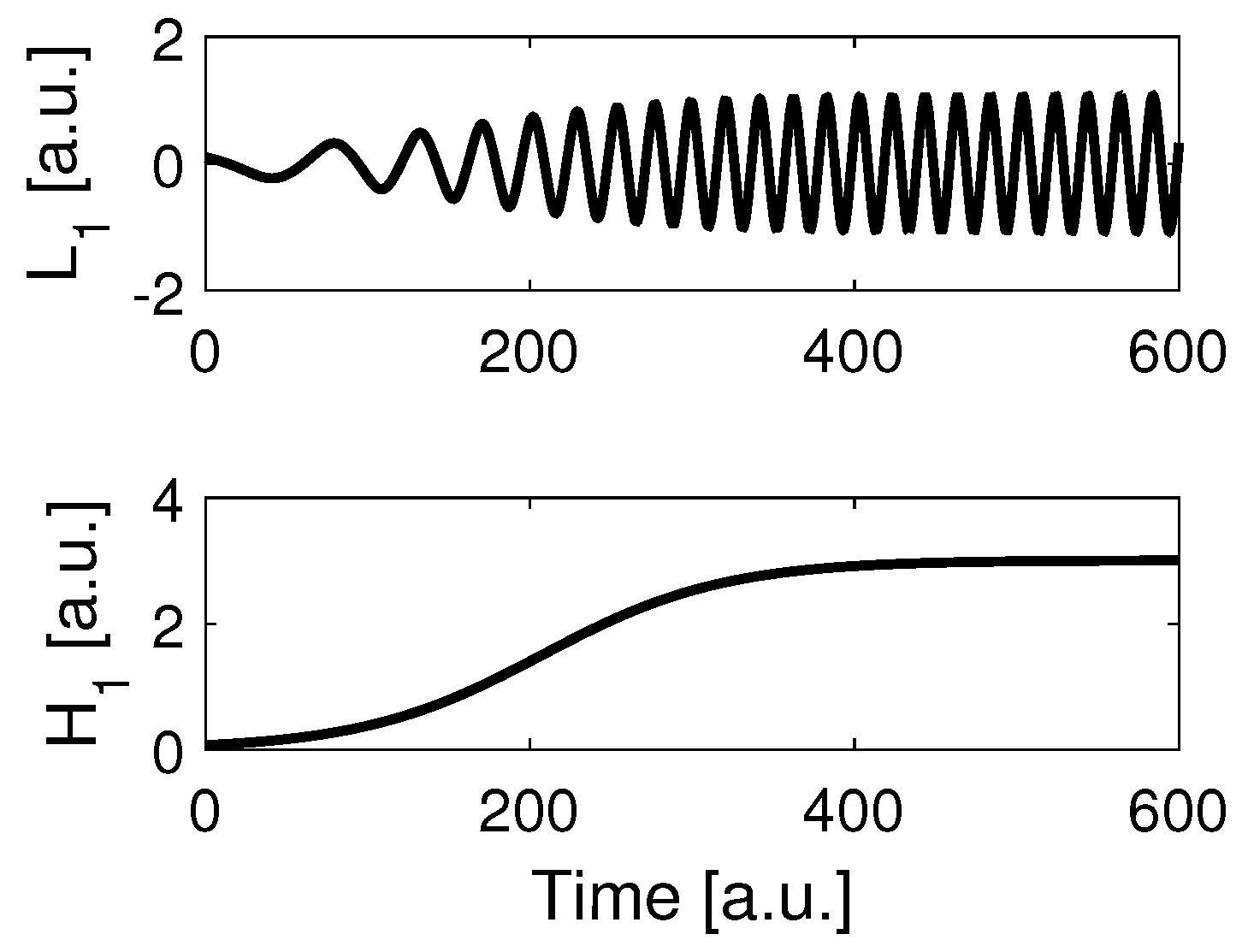
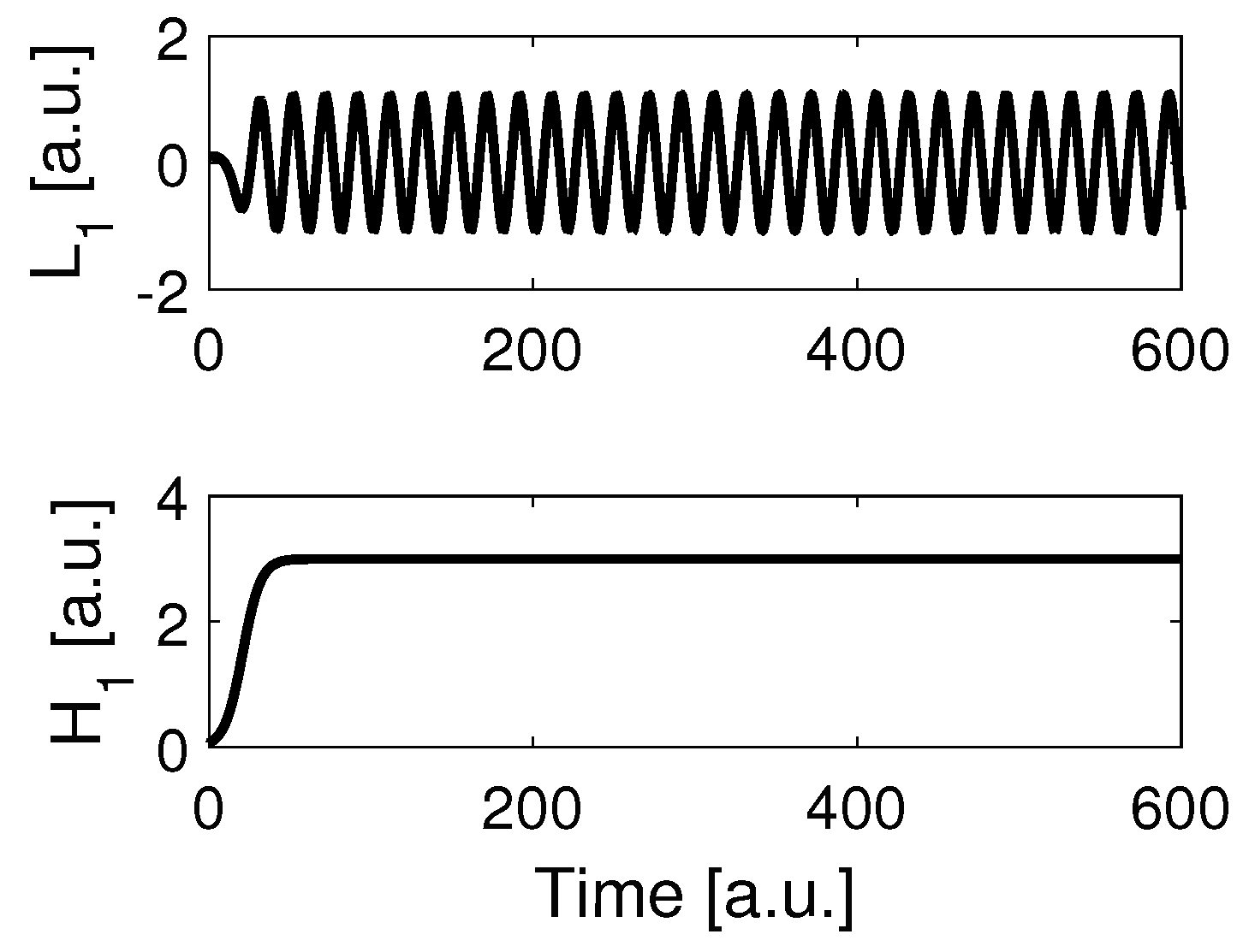
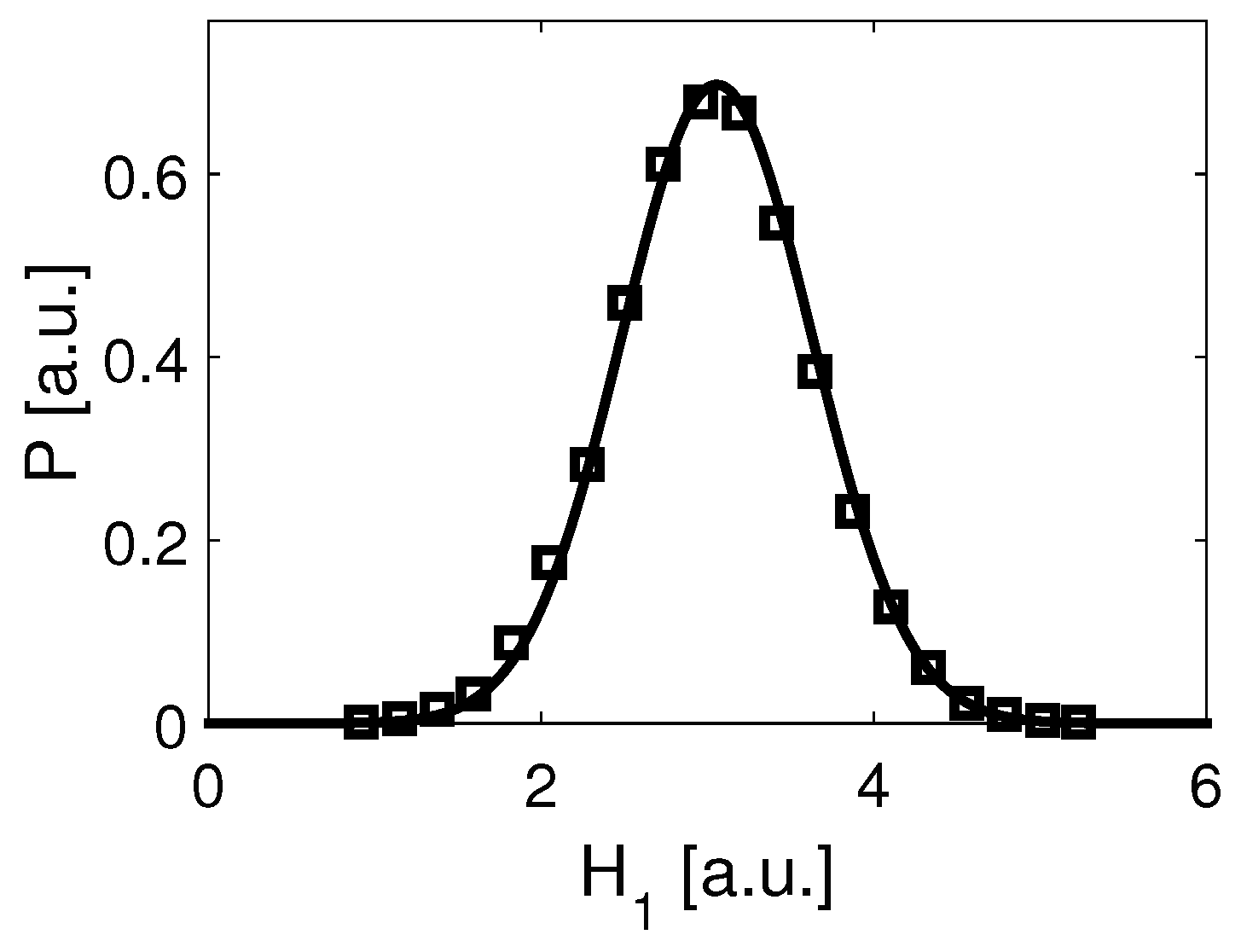
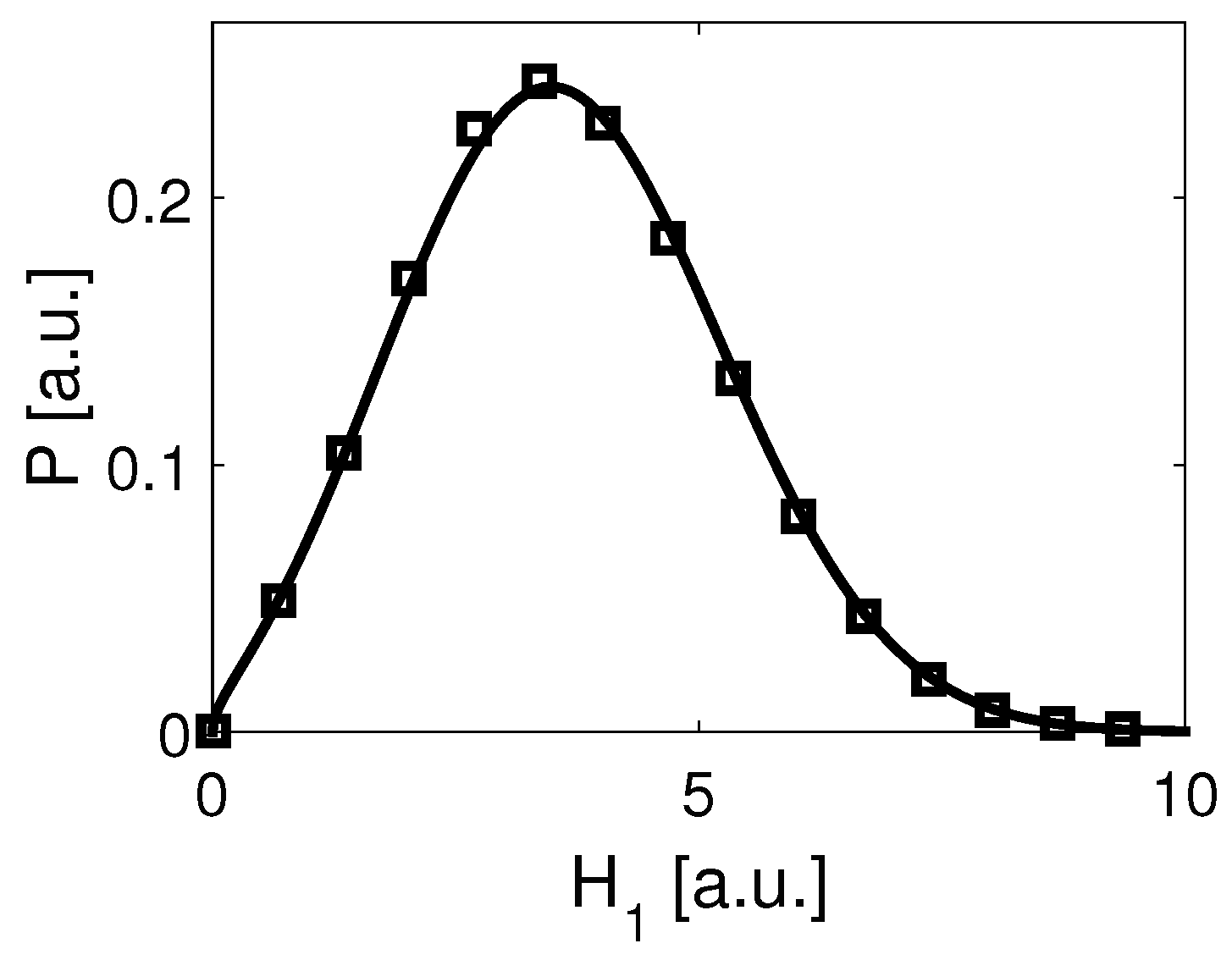
So far, we have discussed purely-dissipative systems and stochastic systems within the framework of the classical Boltzmann–Gibbs–Shannon thermostatistics. Let us turn next to an example of an active stochastic Nambu system. Nambu mentioned in his seminal study on Nambu mechanics that the Euler equations of the spinning top can be cast into the form of Equation (1). The freely rotating spinning top can be considered as a Nambu system. In two previous studies, a stochastic, active version of a spinning top has been introduced exploiting the Nambu mechanics approach [7,19]. This proposed stochastic active spinning top has been discussed from the perspective of classical Boltzmann–Gibbs–Shannon thermostatistics. In what follows, we will introduce a non-extensive variant based on the Tsallis entropy of the stochastic active spinning top proposed in the aforementioned earlier studies [7,19]. Moreover, in this context, the thermodynamic state variables $F_{\mathrm{NL}}$, $U_{\mathrm{NL}}$ and S will be introduced, and the corresponding thermodynamic perspective will be taken as a departure point.

The dynamics of a spinning top can conveniently be described by means of the three-dimensional angular momentum vector $\mathbf{L}=(L_1,L_2,L_3)$. Let $I_1$, $I_2$ and $I_3$ denote the principle inertia moments of the top. Then, the evolution equation for $\mathbf{L}$ is given by the Euler equation:

$$\frac{\mathrm{d}}{\mathrm{d}t}\mathbf{L}=\mathbf{L}\times \left(\begin{array}{c}{L}_1/I_1\\ L_2/I_2\\ L_3/I_3\end{array}\right)=\mathbf{L}\times R\mathbf{L},$$

(61)

where we have introduced the diagonal matrix:

$$R=\left(\begin{array}{ccc}1/I_1& 0& 0\\ 0& 1/I_2& 0\\ 0& 0& 1/I_3\end{array}\right)$$

(62)

of “inverse” inertia coefficients. Let us put $n=3$ and $\mathbf{r}=\mathbf{L}$. Moreover, we introduce $H_1$ defined by half of the squared amount of the angular momentum and $H_2$ given by the kinetic energy as invariants:

$$H_1=\frac{{\mathbf{L}}^2}{2},H_2=\frac{1}{2}\left(\frac{L_1^2}{I_1}+\frac{L_2^2}{I_2}+\frac{L_3^2}{I_3}\right)=\frac{1}{2}\mathbf{L}R\mathbf{L}.$$

(63)

Then, substituting Equation (63) together with Equation (53) into the Nambu Equation (1), we re-obtain the Euler Equation (61). In doing so, it can be shown that the spinning top is a Nambu system.

We consider next an active stochastic variant of the spinning tops dynamics (61) featuring non-extensive thermostatistics. To this end, we put ${\nabla }_D=\nabla =(\partial /\partial L_1,\partial /\partial L_2,\partial /\partial L_3)$ and $M=\gamma E$ as in Equation (56). Furthermore, we put:

$$\begin{array}{ccc}\hfill S& =& S_{\mathrm{T}},\hfill \\ \hfill g(H_1,H_2)=\frac{A_1}{2}{(H_1-B_1)}^2+\frac{A_2}{2}{(H_2-B_2)}^2\Rightarrow U_{\mathrm{NE}}& =& \int gP{\mathrm{d}}^{3}L,\hfill \\ \hfill F_{\mathrm{NE}}& =& U_{\mathrm{NE}}-\theta S_{\mathrm{T}}\hfill \end{array}$$

(64)

with $A_1,A_2\ge 0$. Substituting Equation (64) together with ${\nabla }_D=\nabla$ and $M=\gamma E$ into Equation (11) yields:

$$\frac{\partial }{\partial t}P=-\nabla \left\{[\mathbf{L}\times R\mathbf{L}-{\gamma }_1\mathbf{L}(H_1-B_1)-{\gamma }_{2}R\mathbf{L}(H_2-B_2)]P\right\}+\Delta D{P}^q$$

(65)

with $\Delta ={\nabla }^2$ and $D=\gamma \theta$ again. Moreover, we have defined ${\gamma }_1=\gamma A_1$ and ${\gamma }_2=\gamma A_2$. The Fokker–Planck Equation (65) defines the evolution of the probability density $P(\mathbf{L},t)$. For $q=1$, the model reduces to the stochastic version proposed earlier in the literature [7] describing a linear partial differential equation, that is, an ordinary Fokker–Planck equation. In contrast, for $q\ne 1$, the model is described by a nonlinear partial differential equation.

In order to highlight the active nature of the model (65), we would like to point out that in the “zero temperature limit” given by $\theta =0$, we have an H-theorem for g; see Section 2.4. In particular, for $A_2=0$, this implies that in the limiting case $t\to \infty$, the angular momentum $\mathbf{L}$ approaches in the amount the value $\sqrt{2B_1}$, such that $H_1=B_1$. Likewise, for $A_1=0$, it follows that the kinetic energy approaches in the long time limit the parameter value $B_2$. In this sense, the model features a pumping mechanisms (i.e., negative damping) that leads to an increase of angular momentum ($A_1>0$, $A_2=0$) or kinetic energy ($A_1=0$, $A_2>0$).

Stochastic trajectories $\mathbf{L}\left(t\right)$ can be computed by means of [38]:

$$\frac{\mathrm{d}}{\mathrm{d}t}\mathbf{L}=\mathbf{L}\times R\mathbf{L}-{\gamma }_1\mathbf{L}(H_1-B_1)-{\gamma }_{2}R\mathbf{L}(H_2-B_2)+\sqrt{D}{\left.P^{(q-1)/2}(\mathbf{u},t)\right|}_{\mathbf{u}=\mathbf{L}\left(t\right)}\mathsf{\Gamma }\left(t\right),$$

(66)

where $\mathsf{\Gamma }\left(t\right)$ denotes the three-dimensional Langevin force mentioned in the previous example of Section 3.2. The stochastic evolution Equation (66) can be interpreted in two alternative ways. First, we may consider Equation (66) as part of a two-tiered (or two-layered [38]) description of the stochastic trajectories $\mathbf{L}\left(t\right)$. Accordingly, first, the Fokker–Planck Equation (65) is solved in the time-interval $[t_1,t_2]$ of interest (tier one). In doing so, $P(\mathbf{L},t)$ is obtained. Subsequently, the solution $P(\mathbf{L},t)$ is substituted into Equation (66). In this case, Equation (66) corresponds to a non-autonomous, multiplicative noise Langevin equation (tier two) interpreted according to Ito calculus. Alternative to this two-tiered interpretation, Equation (66) can be regarded as a self-consistent Langevin equation [38]. In line with this alternative interpretation, the probability density $P(\mathbf{L},t)$ is computed from trajectories $\mathbf{L}\left(t\right)$ like $P(\mathbf{u},t)=〈\delta (\mathbf{u}-\mathbf{L}(t\left)\right)〉$. However, the evolution of the trajectories $\mathbf{L}\left(t\right)$ in turn depends on $P(\mathbf{L},t)$.

Depending on the parameter q, the stationary probability density assumes one of the forms defined by Equations (28), (29) and (30) with g given by Equation (64). For $q\in (0,1)$, we obtain:

$$P\left(\mathbf{L}\right)={\left(\frac{q}{(1-q){\left(2\theta \right)}^{-1}(A_1{(H_1\left(\mathbf{L}\right)-B_1)}^2+A_2{(H_2\left(\mathbf{L}\right)-B_2)}^2-2\mu )+1}\right)}^{1/(1-q)}.$$

(67)

For $q=1$, we get:

$$P\left(\mathbf{L}\right)=\frac{1}{Z}\exp \left\{-\frac{A_1{(H_1\left(\mathbf{L}\right)-B_1)}^2+A_2{(H_2\left(\mathbf{L}\right)-B_2)}^2}{2\theta }\right\}$$

(68)

with $Z=\exp \{1-(\mu /\theta \left)\right\}$ as in Equation (28).

For $q>1$, we obtain:

$$P\left(\mathbf{L}\right)={\left(\frac{{[(q-1){\left(2\theta \right)}^{-1}(2\mu -A_1{(H_1\left(\mathbf{L}\right)-B_1)}^2+A_2{(H_2\left(\mathbf{L}\right)-B_2)}^2)+1]}_{+}}{q}\right)}^{1/(q-1)}.$$

(69)

In order to arrive at a more precise interpretation of the stationary distributions, we may discuss the stationary distribution in appropriately-defined one-dimensional spaces related to the invariants $H_1$ and $H_2$, rather than in the original state space [57,58,59]. That is, we define the distributions:

$$P_j\left(\xi \right)=〈\delta (\xi -H_j\left(\mathbf{L}\right))〉=\int \delta (\xi -H_j\left(\mathbf{L}\right))P\left(\mathbf{L}\right){\mathrm{d}}^{3}L$$

(70)

for $j=1,2$. In order to reduce the number of symbols, we may consider $H_j$ both as a coordinate and a random variable, depending on its context. Accordingly, we replace ξ by $H_j$ in Equation (70) and define the distributions of the invariants like:

$$P_j\left(H_j\right)=〈\delta (H_j-H_j\left(\mathbf{L}\right))〉=\int \delta (H_j-H_j\left(\mathbf{L}\right))P\left(\mathbf{L}\right){\mathrm{d}}^{3}L.$$

(71)

For illustration purposes, let us focus on an active system that features a pumping mechanism that makes the angular moment become asymptotically stable at the amount $\sqrt{2B_1}$ (in the deterministic case $\theta =0$). That is, we put $A_2=0$. From Equation (71) and Equations (67)–(69), we obtain the distributions:

$$P_1\left(H_1\right)=\frac{\sqrt{H_1}}{Z^{\prime }}{\left(\frac{q}{(1-q){\left(2\theta \right)}^{-1}(A_1{(H_1-B_1)}^2-2\mu )+1}\right)}^{1/(1-q)}$$

(72)

for $q\in (0,1)$,

$$P_1\left(H_1\right)=\frac{\sqrt{H_1}}{Z^{\prime }Z}\exp \left\{-\frac{A_1{(H_1-B_1)}^2}{2\theta }\right\}=\frac{\sqrt{H_1}}{Z^{\prime }Z}\exp \left\{-\frac{{\gamma }_1{(H_1-B_1)}^2}{2D}\right\}$$

(73)

for $q=1$ with $Z=\int \exp \{-A_1{(H_1-B_1)}^2/\left(2\theta \right)\}{\mathrm{d}}^{3}L$ and:

$$P_1\left(H_1\right)=\frac{\sqrt{H_1}}{Z^{\prime }}{\left(\frac{{[(q-1){\left(2\theta \right)}^{-1}(2\mu -A_1{(H_1-B_1)}^2)+1]}_{+}}{q}\right)}^{1/(q-1)}$$

(74)

for $q>1$. In Equations (72)–(74), the pre-factor $\sqrt{H_1}/Z^{\prime }$ is a re-normalization factor that occurs due to the fact that we transform distributions from a three-dimensional state space to a one-dimensional one. Roughly speaking, we put $P_1\left(H_1\right)\mathrm{d}{H}_1=P\left(\mathbf{L}\right){\mathrm{d}}^{3}L$ and express the three-dimensional state space element ${\mathrm{d}}^{3}L$ like ${\mathrm{d}}^{3}L=2{\left(\sqrt{2}\right)}^{-1}{\left|\mathbf{L}\right|}^2\mathrm{d}\left|\mathbf{L}\right|/Z^{\prime }={\left(\sqrt{2}\right)}^{-1}\left|\mathbf{L}\right|\mathrm{d}{H}_1/Z^{\prime }=\sqrt{H_1}\mathrm{d}{H}_1/Z^{\prime }$.

The distributions (72)–(74) can be characterized as follows. For $q\in (0,1)$, the energy distribution is a power law distribution. The probability density of the pseudo-invariant $H_1$ decays like $\sqrt{H_1}{H}_1^{2/(1-q)}=H_1^{1/(1-q)}$ for sufficiently large values. Since we have ${\left|\mathbf{L}\right|}^2=2H_1$, the probability density of the squared angular moment $\left|\mathbf{L}\right|$ behaves qualitatively in the same way. For $q=1$, the distribution would be a truncated normal distribution (truncated at $H_1=0$) with a maximum at $H_1=B_1$ if we ignore the pre-factor $\sqrt{H_1}/Z^{\prime }$. This truncated normal distribution has been studied in detail (both in theoretical and experimental works) in the context of the standard canonical-dissipative limit-cycle oscillator [36,44,57,58,60,61]. Taking the pre-factor $\sqrt{H_1}/Z^{\prime }$ into account, the truncated normal distribution becomes distorted. For $q>1$, the distribution is a cutoff distribution. It is useful to introduce the parameter ${\mu }_{\mathrm{eff}}=\mu +\theta /(q-1)$, such that Equation (74) reduces to:

$$P_1\left(H_1\right)=\frac{\sqrt{H_1}}{Z^{\prime }}{\left(\frac{(q-1){\left(2\theta \right)}^{-1}{[2{\mu }_{\mathrm{eff}}-A_1{(H_1-B_1)}^2]}_{+}}{q}\right)}^{1/(q-1)}.$$

(75)

From Equation (75), it is clear that the shape of the distribution follows an inverted U with a maximum at $H_1=B_1$. The distribution exhibits two cutoff points at $H_{1\pm }=B_1\pm \sqrt{2{\mu }_{\mathrm{eff}}/A_2}$ provided that $B_1-\sqrt{2{\mu }_{\mathrm{eff}}/A_1}\ge 0$ holds. If $B_1-\sqrt{2{\mu }_{\mathrm{eff}}/A_1}<0$ holds, then the cutoff points are located at $H_{1+}=B_1+\sqrt{2{\mu }_{\mathrm{eff}}/A_1}$ and $H_{1-}=0$. The distribution assumes finite values in the interval $(H_{1-},H_{1+})$ (which is the so-called “support” of the distribution) and is zero otherwise.

3.4. Numerics

In order to illustrate the active nature of the canonical-dissipative spinning top model (65), we solved numerically the corresponding Langevin Equation (66). We focused on the Boltzmann-Gibbs-Shannon case $q=1$ and a pumping mechanism that stabilized the amount of angular moment ($A_1>0$, $A_2=0$). Figure 1 and Figure 2 show one component of $\mathbf{L}$, as well as the pseudo-invariant $H_1$ as functions of time for two different parameters ${\gamma }_1$ in the deterministic case (zero temperature limit $\theta =0\Rightarrow D=0$). As expected from our general considerations in Section 2.4, the pseudo-invariant $H_1$ converged to the stationary value $B_1$. The relaxation time towards stationarity became shorter when ${\gamma }_1$ was increased. That is, ${\gamma }_1$ determined the characteristic time scale of the transient period. This interpretation of ${\gamma }_1$ can also be seen from Equation (36). Substituting $g=A_1\delta H_1^2/2$ with $\delta H_1=H_1-B_1$ into Equation (36) (together with ${\nabla }_D=\nabla$), we obtain:

$$\frac{\mathrm{d}}{\mathrm{d}t}\delta H_1=-\gamma A_1{(\nabla H_1)}^2{\left(\delta H_1\right)}^2=-{\gamma }_1{(\nabla H_1)}^2{\left(\delta H_1\right)}^2.$$

(76)

Accordingly, the difference $\delta H_1$ between $H_1$ and its fixed point value $B_1$ decays faster when ${\gamma }_1$ is larger, which is what we found in the numerical simulations.

The stationary probability density (73) is shown in Figure 3 and Figure 4 for two different diffusion constants. For a relatively small diffusion constant, the pre-factor $\sqrt{H_1}$ has relatively little impact, and the distribution resembles a normal distribution; see Figure 3. In contrast, if the diffusion constant is sufficiently larger, the distorting impact of the pre-factor $\sqrt{H_1}$ becomes dominant, and the shape of the distribution qualitatively differs from a normal distribution; see Figure 4. Irrespective of D, the distribution of the pseudo-invariant $H_1$ corresponding to the squared angular moment is unimodal and exhibits its maximum at a value $H_1>0$. This peak at a value different from the “ground state value” $H_1=0$ indicates that the system is an active system rather than a purely dissipative one [62].

4. Discussion

4.1. Invariants of Nambu Dynamics as Pseudo-Invariants

We proposed a stochastic framework to discuss active Nambu systems that allows one to address thermodynamic state variables, on the one hand, and generalized entropic measures, on the other hand. The approach is based on classical Nambu mechanics. Consequently, for an n-dimensional system, there are $n-1$ functions $H_1,\cdots ,H_{n-1}$ that act as invariants in the classical Nambu system. However, in the stochastic, active variant of that system, the functions $H_1,\cdots ,H_{n-1}$ vary over time. There are two reasons.

First, in line with the so-called canonical-dissipative modeling effort for active systems, the systems feature a pumping mechanism that makes sure that at least one of the functions $H_1,\cdots ,H_{n-1}$ approaches a fixed point value. That is, while in classical Nambu mechanics, the function values $H_1,\cdots ,H_{n-1}$ are determined by the initial conditions (i.e., initial values of the state vector $(r_1,\cdots ,r_n)$); for active Nambu systems, at least one function $H_j$ converges to a fixed point value $B_j$ and in doing so assumes in the long time limit a value that does not depend on the initial conditions. Figure 1 and Figure 2 illustrate this transient dynamics. After the transient period, we have $|H_j-B_j|<C$, where $C>0$ can be made arbitrarily small. In this case, variation in time of $H_j$ may be considered as being negligibly small, and we may refer to this domain as the stationary domain. We may say that in the stationary domain, the system has approached an attractor defined by the original Nambu system that does not feature the pumping mechanism. In this context, note that the phrase “pumping mechanisms” actually refers to a pumping and damping mechanism. For example, if the initial conditions are such that $H_j>B_j$, then $H_j$ decays towards $B_j$.

Second, taking fluctuating forces into account associated with the entropic form S, due to the impact of these fluctuating forces, the functions $H_1,\cdots ,H_{n-1}$ vary over time in an erratic fashion. This holds both in the transient and stationary domain. In the stationary domain, the fluctuations can be illustrated by means of the stationary probability density $P_j\left(H_j\right)$. We demonstrated the erratic variations of the functions $H_1,\cdots ,H_{n-1}$ for a stochastic, active spinning top model involving the functions $H_1$ and $H_2$, where $H_1$ corresponds to half of the squared amount of the angular momentum. The probability density $P_1\left(H_1\right)$ is shown in Figure 3 and Figure 4 for two systems that differ with respect to the “strength” of the impact of the fluctuating force (as quantified by the diffusion coefficient).

In view of these consideration, it might be useful to refer to the functions $H_1,\cdots ,H_{n-1}$ occurring in stochastic, active Nambu systems described by Equation (9) as pseudo-invariants rather than invariants. The functions $H_1,\cdots ,H_{n-1}$ of Equation (9) are pseudo-invariants in the sense that in the limit $t\to \infty$ and in the “zero temperature limit” $\theta \to 0$, the variants over time of these functions become negligibly small.

4.2. Active, Stochastic Systems and Generalized, Non-Extensive Entropic Measures

Let us motivate the utilization of generalized entropy measures of the form (3) and in particular the Tsallis entropy (6) for active systems. To this end, we would like to focus on active systems that describe human and animal behavior and in particular the motor control system of humans and animals.

The Boltzmann–Gibbs–Shannon entropy is an extensive measure. That is, when applied to many body systems, it does not account for long-range interactions between individual subsystems of many body systems. While for many applications (for example in the statistical mechanics description of ideal gases), such long-range interaction can be neglected, human and animal behavior may results from a plenitude of interacting components that feature long-range interactions. For example, on the neuronal level, neurons in the motor cortex may need to synchronize their activity in order to produce a descending signal that controls limb movement. The axonal connections between these neurons may be considered as representing long-range connections rather than local connections. The Tsallis entropy (6) has been proposed with this goal in mind to account for non-extensivity effect as a result of long-range interactions between components [39].

Second, the control of human and animal motor behavior involves several subsystems, such as the neural systems, the muscular system and the human and animal body as such (i.e., the system of the limbs). These subsystem feature again subsystems. For example, within the neural system, we may distinguish between processes at the synapses, the membrane and in the axons. The point that we would like to make here is that the human and animal motor control system from a mechanistic (microscopic, bottom-up) perspective involves various components that are likely to evolve on different characteristic time scales. To model explicitly all of these components is a challenging task. Alternatively, one may think of using stochastic models that are able to capture processes that take place at different levels of consideration at the same time. Scale independent models as described for example by the Levy distribution are models that exhibit this feature. This kind of model is known to exhibit power law distributions rather than normal distributions or Boltzmann distributions. As we have shown in Section 3, when taking general entropic forms into account, the shape of the stationary distributions is determined by the entropic form. In particular, using a non-extensive thermostatistic approach based on the Tsallis entropy (6), for non-extensivity parameters $q<1$, the power law distribution can be modeled; see Section 3.2. In other words, using a generalized thermostatistic approach that leads to a stationary power law distribution allows us to capture in a crude way that active biological systems and in particular human and animal motor control systems involve various subcomponents that are likely to act on different characteristic time scales.

Let us reiterate that in view of the considerations made above, the proposed stochastic Nambu mechanics models are promising models to capture on appropriately-defined descriptive, macroscopic levels characteristic properties of biological systems (e.g., that their observables satisfy power law distributions). In fact, for the migration (cell motion) of certain bacteria, experimental evidence has been found that the bacteria velocity scores are distributed in a certain range according to a power law [63]. It has further been suggested that the absolute velocity scores satisfy a Tsallis distribution similar to the power law distribution (29). In short, while a stochastic model of the form (9) may not be able to provide a mechanistic account of the many interacting components of a biological system under consideration, the model might be used as a phenomenological model to address certain macroscopic aspects of the system. If so, the benefit of the approach outlined above is that thermodynamic variables can be introduced in a well-defined manner such that the performance of the system under consideration can be studied from a thermodynamical perspective.

Having argued that the case $q<1$ in non-extensive thermostatistics can help us to build more realistic models of active systems, one can also argue that the alternative case $q>1$ has relevance for our understanding of active systems [64]. Active systems as frequently been found in biology are in general limited in their performance measures. For example, humans and animals can run just so fast, and translational and rotational limb movement can be performed only up to certain maximal values of speed and angular velocity. Cutoff distributions can take these limitations into account. Modeling human and animal behavior by means of cutoff distributions implies that we acknowledge that human behavior is subjected to limits. Accordingly, the observable related to the behavior of interest will not assume values beyond certain limits. The probability to find observable values beyond these limits equals zero.

The cases $q<1$ and $q>1$ are conflicting alternatives. When modeling a certain phenomenon of interest, one may give priority to either one of the two aforementioned aspects motivating the utilization of non-extensive thermostatistics with $q<1$ or $q>1$. Future efforts may be directed to combine both aspects in a single model.

5. Conclusions

Stochastic Nambu mechanics models provide a relatively novel theoretical framework to address systems in the life sciences from a physics perspective. This perspective includes both dynamic and thermodynamic aspects. Interestingly, the approach does not aim to establish a new physics of the animate world that is separated from the physics concerned with the inanimate world. Rather, as has been demonstrated above, the stochastic Nambu mechanics perspective is sufficiently broad to address both active systems as typically observed in the life sciences and equilibrium or close to equilibrium systems as frequently studied in classical physics. From a mathematical point of view, the stochastic models under consideration can be described by nonlinear partial differential equations for probability densities. Although in general, it is difficult to determine the properties of equations of this kind, the underlying thermodynamic aspects of the theory turns out to provide tools to analyze solutions. For example, we were able to determine certain properties of transient and stationary probability densities of the stochastic Nambu mechanics models. Importantly, we illustrated that the type of the nonlinearity of a partial differential equation under consideration corresponds to a certain type of an entropy measure. It is this link between the type of the entropy measure and the type of the nonlinearity that endows the proposed theoretical framework with powerful tools that can be used in applications to experimental data and theory-building.

References

1. Nambu, Y. Generalized Hamiltonian dynamics. Phys. Rev. D 1973, 7, 2405–2412. [Google Scholar] [CrossRef]
2. Pandit, S.A.; Gangal, A.D. On generalized Nambu mechanics. J. Phys. A 1998, 31, 2899–2912. [Google Scholar] [CrossRef]
3. Plastino, A.R.; Plastino, A.; da Silva, L.R.; Casas, M. Dynamic thermostatting, divergenceless phase-space flows, and KBB systems. Physica A 1999, 271, 343–356. [Google Scholar] [CrossRef]
4. Roston, G.B.; Plastino, A.R.; Casas, M.; Plastino, A.; da Silva, L.R. Dynamic thermostatting and statistical ensemble. Eur. Phys. J. B 2005, 48, 87–93. [Google Scholar] [CrossRef]
5. Steeb, W.H.; Euler, N. A note on Nambu mechanics. Il Nuovo Cim. B 1991, 106, 263–272. [Google Scholar] [CrossRef]
6. Tegmen, A. Momentum map and action-angle variables for Nambu mechanics. Czechoslov. J. Phys. 2004, 54, 749–757. [Google Scholar] [CrossRef]
7. Frank, T.D. A Fokker-Planck approach to canonical-dissipative Nambu systems: With an application to human motor control during dynamic haptic perception. Phys. Lett. A 2010, 374, 3136–3142. [Google Scholar] [CrossRef]
8. Yamaleev, R.M. Generalized Newtonian equations of motion. Ann. Phys. 1999, 277, 1–18. [Google Scholar] [CrossRef]
9. Yamaleev, R.M. Relativistic equations of motion within Nambu’s formalism of dynamics. Ann. Phys. 2000, 285, 141–160. [Google Scholar] [CrossRef]
10. Molgado, A.; Rodriguez, A. Mapping between the dynamic and mechanical properties of the relativistic oscillator and Euler free rigid body. J. Nonlinear Math. Phys. 2007, 14, 534–547. [Google Scholar] [CrossRef]
11. Codriansky, S.; Bernardo, C.A.G.; Aglaee, A.; Carrillo, F.; Castellanos, J.; Pereira, G.; Perez, J. Developments in Nambu mechanics. J. Phys. A 1994, 27, 2565–2578. [Google Scholar] [CrossRef]
12. Plastino, A.R.; Plastino, A. Statistical treatment of autonomous systems with divergenceless flow. Physica A 1996, 232, 458–476. [Google Scholar] [CrossRef]
13. Chatterjee, R. Dynamical symmetries and Nambu mechanics. Lett. Math. Phys. 1996, 36, 117–126. [Google Scholar] [CrossRef] [Green Version]
14. Nutku, Y. Quantization with maximally degenerate Poisson brackets: The harmonic oscillator. J. Phys. A 2003, 36, 7559–7567. [Google Scholar] [CrossRef]
15. Baleanu, D. Angular momentum and Killing-Yano tensors. Proc. Inst. Math. NSA Ukraine 2004, 50, 611–616. [Google Scholar] [CrossRef]
16. Curtright, T.L.; Zachos, C. Deformation quantization of superintegrable systems and Nambu mechanics. New J. Phys. 2002, 4. [Google Scholar] [CrossRef]
17. Curtright, T.L.; Zachos, C. Classic and quantum Nambu mechanics. Phys. Rev. D 2002, 68, 085001. [Google Scholar] [CrossRef]
18. Zachos, C. Membranes and consistent quantization of Nambu dynamics. Phys. Lett. B 2003, 570, 82–88. [Google Scholar] [CrossRef]
19. Frank, T.D. Active systems with Nambu dynamics: With applications to rod wielding for haptic length perception and self-propagating systems on two-spheres. Eur. Phys. J. B 2010, 74, 195–203. [Google Scholar] [CrossRef]
20. Hirayama, M. Realization of Nambu mechanics: A particle interacting with an SU(2) monopole. Phys. Rev. D 1977, 16, 530. [Google Scholar] [CrossRef]
21. Yamaleev, R.M. Generalized Lorentz-force equations. Ann. Phys. 2001, 292, 157–178. [Google Scholar] [CrossRef]
22. Pletnev, N.G. Fillipov-Nambu n-algebras relevant to physics. Sib. Electron. Math. Rep. 2009, 6, 272–311. [Google Scholar]
23. Gonera, C.; Nuktu, Y. Super-integrable Calogero-type systems admit maximal number of Poisson structures. Phys. Lett. A 2001, 285, 301–306. [Google Scholar] [CrossRef]
24. Tegmen, A.; Vercin, A. Superintegrable systems, multi-Hamiltonian structures and Nambu mechanics in an arbitrary dimension. Int. J. Mod. Phys. B 2004, 19, 393–409. [Google Scholar] [CrossRef]
25. Guha, P. Application of Nambu mechanics to systems of hydrodynamical type II. J. Nonlinear Math. Phys. 2004, 11, 223–232. [Google Scholar] [CrossRef]
26. Müller, R.; Nevir, P. A geometric application of Nambu mechanics: The motion of three point vortices in the plane. J. Phys. A 2014, 47, 105201. [Google Scholar] [CrossRef]
27. Roupas, Z. Phase space geometry and chaotic attractors in dissipative Nambu mechanics. J. Phys. A 2012, 45, 195101. [Google Scholar] [CrossRef]
28. Mathis, W.; Stahl, D.; Mathis, R. Oscillator synthesis based on Nambu mechanics and canonical dissipative damping. In Proceedings of the 21st European Conference on Circuit Theory and Design (ECCTD 2013), Dresden, Germany, 8–12 September 2013.
29. Mathis, W.; Mathis, R. Dissipative Nambu systems and oscillator circuit design. Nonlinear Theory Appl. IEICE 2014, 5, 259–271. [Google Scholar] [CrossRef]
30. Frank, T.D. Unifying mass-action kinetics and Newtonian mechanics by means of Nambu brackts. J. Biol. Phys. 2011, 37, 375–385. [Google Scholar] [CrossRef] [PubMed]
31. Frank, T.D. Nambu brackt formulation of nonlinear biochemical reactions beyond elementary mass action kinetics. J. Nonlinear Math. Phys. 2012, 19, 81–97. [Google Scholar] [CrossRef]
32. Mongkolsakulvong, S.; Chaikhan, P.; Frank, T.D. Oscillatory nonequilibrium Nambu systems: The canonical-dissipative Yamaleev oscillator. Eur. Phys. J. B 2012, 85. [Google Scholar] [CrossRef]
33. Chaikhan, P.; Frank, T.D.; Mongkolsakulvong, S. In-phase and anti-phase synchronization in an active Nambu mechanics system. Acta Mech. 2016, 10, 2703–2717. [Google Scholar] [CrossRef]
34. Gordon, J.M.; Kim, S.; Frank, T.D. Linear non-equilibrium thermodynamics of human voluntary behavior: A canonical-dissipative Fokker-Planck equation approach involving potentials beyond the harmonic case. Condens. Matter Phys. 2016, 19, 1–6. [Google Scholar] [CrossRef]
35. Schweitzer, F. Brownian Agents and Active Particles; Springer: Berlin/Heidelberg, Germany, 2003. [Google Scholar]
36. Romanczuk, P.; Bär, M.; Ebeling, W.; Lindner, B.; Schimansky-Geier, L. Active Brownian particles: From individual to collective stochastic dynamics. Eur. Phys. J. Spec. Top. 2012, 202, 1–162. [Google Scholar] [CrossRef]
37. Haken, H. Synergetics: An Introduction; Springer: Berlin/Heidelberg, Germany, 1977. [Google Scholar]
38. Frank, T.D. Nonlinear Fokker-Planck Equations: Fundamentals and Applications; Springer: Berlin/Heidelberg, Germany, 2005. [Google Scholar]
39. Tsallis, C. Possible generalization of Boltzmann-Gibbs statistics. J. Stat. Phys. 1988, 52, 479–487. [Google Scholar] [CrossRef]
40. Tsallis, C. Non-extensive thermostatistics: Brief review and comment. Physica A 1995, 221, 227–290. [Google Scholar] [CrossRef]
41. Abe, S.; Okamoto, Y. Nonextensive Statistical Mechanics and Its Applications; Springer: Berlin/Heidelberg, Germany, 2001. [Google Scholar]
42. Haken, H. Distribution function for classical and quantum systems far from thermal equilibrium. Z. Phys. 1973, 263, 267–282. [Google Scholar] [CrossRef]
43. Graham, R. Statistical Theory of Instabilities in Stationary Nonequilibrium Systems with Applications to Lasers and Nonlinear Optics. In Springer Tracts in Modern Physics; Höhler, G., Ed.; Springer: Berlin/Heidelberg, Germany, 1973; Volume 66, pp. 1–97. [Google Scholar]
44. Ebeling, W.; Sokolov, I.M. Statistical Thermodynamics and Stochastic Theory of Nonequilibrium Systems; World Scientific: Singapore, 2004. [Google Scholar]
45. Plastino, A.R.; Plastino, A. Non-extensive statistical mechanics and generalized Fokker-Planck equation. Physica A 1995, 222, 347–354. [Google Scholar] [CrossRef]
46. Crank, J. The Mathematics of Diffusion; Clarendon Press: Oxford, UK, 1975. [Google Scholar]
47. Peletier, L.A. The Porous Media Equation; Applications of Nonlinear Analysis in the Physical Science; Amann, H., Bazley, N., Kirchgässner, K., Eds.; Pitman Advanced Publishing Program: Boston, MA, USA, 1981; pp. 229–241. [Google Scholar]
48. Barenblatt, G.I.; Entov, V.M.; Ryzhik, V.M. Theory of Fluid Flows through Natural Rocks; Kluwer Academic Publisher: Dordrecht, The Netherlands, 1990. [Google Scholar]
49. Risken, H. The Fokker-Planck Equation. Methods of Solution and Applications; Springer: Berlin/Heidelberg, Germany, 1989. [Google Scholar]
50. Kaniadakis, G. H-theorem and generalized entropies within the framework of nonlinear kinetics. Phys. Lett. A 2001, 288, 283–291. [Google Scholar] [CrossRef]
51. Shiino, M. Free energies based on generalized entropies and H-theorems for nonlinear Fokker-Planck equations. J. Math. Phys. 2001, 42, 2540–2553. [Google Scholar] [CrossRef]
52. Frank, T.D.; Daffertshofer, A. H-theorem for nonlinear Fokker-Planck equations related to generalized thermostatistics. Physica A 2001, 295, 455–474. [Google Scholar] [CrossRef]
53. Chavanis, P.H. Generalized Fokker-Planck equations and effective thermodynamics. Physica A 2004, 340, 57–65. [Google Scholar] [CrossRef]
54. Schwämmle, V.; Nobre, F.D.; Curado, E. Consequences of the H-theorem for nonlinear Fokker-Planck equations. Phys. Rev. E 2007, 76, 041123. [Google Scholar] [CrossRef] [PubMed]
55. Frank, T.D. On the boundedness of free energy functionals. Nonlinear Phenom. Complex Syst. 2003, 6, 696–704. [Google Scholar]
56. Dotov, D.G.; Frank, T.D. From the W-method to the canonical-dissipative method for studying uni-manual rhythmic behavior. Motor Control 2011, 15, 550–567. [Google Scholar] [CrossRef] [PubMed]
57. Dotov, D.G.; Kim, S.; Frank, T.D. Non-equilibrium thermodynamical description of rhythmic motion patterns of active systems: A canonical-dissipative approach. BioSystems 2015, 128, 26–36. [Google Scholar] [CrossRef] [PubMed]
58. Kim, S.; Gordon, J.M.; Frank, T.D. Nonequilibrium thermodynamic state variables of human self-paced rhythmic motions: Canonical-dissipative approach, augmented Langevin equation, and entropy maximization. Open Syst. Inf. Dyn. 2015, 22. [Google Scholar] [CrossRef]
59. Mongkolsakulvong, S.; Frank, T.D. Canonical-dissipative limit cycle oscillators with a short-range interaction in phase space. Condens. Matter Phys. 2010, 13, 13001. [Google Scholar] [CrossRef]
60. Frank, T.D. On a moment-based data analysis method for canonical-dissipative oscillator systems. Fluct. Noise Lett. 2010, 9, 69–87. [Google Scholar] [CrossRef]
61. Frank, T.D.; Kim, S.; Dotov, D.G. Canonical-dissipative nonequilibrium energy distributions: Parameter estimation via implicit moment method, implementation and application. Int. J. Mod. Phys. B 2013, 27. [Google Scholar] [CrossRef]
62. Frank, T.D. Virial theorem and non-equilibrium canonical-dissipative distributions characterizing Parkinson tremor. Int. J. Mod. Phys. B 2011, 25, 1465–1469. [Google Scholar] [CrossRef]
63. Bödeker, H.U.; Beta, C.; Frank, T.D.; Bodenschatz, E. Quantitative analysis of random ameboid motion. Europhys. Lett. 2010, 90, 28005. [Google Scholar] [CrossRef]
64. Frank, T.D. Nonextensive cutoff distributions of postural sway for the old and the young. Physica A 2009, 388, 2503–2510. [Google Scholar] [CrossRef]
Figure 1. Trajectories of L 1 (top) and H 1 (bottom) of the active spinning top model without noise. Equation (66) for D = 0 was solved numerically using a Euler forward scheme with a single time step of 0.01 time units. Model parameters: I 1 = 1 . 1 , I 2 = 1 . 3 , I 3 = 1 . 5 , γ 1 = 3 / 1000 , γ 2 = 0 , B 1 = 3 . Initial values: L 1 ( 0 ) = 0 . 1 , L 2 ( 0 ) = 0 . 2 , L 3 ( 0 ) = 0 . 3 .
Entropy 19 00008 g001
Figure 2. As in Figure 1, but for a larger parameter γ 1 : γ 1 = 3 / 100 . Other parameters as in Figure 1: I 1 = 1 . 1 , I 2 = 1 . 3 , I 3 = 1 . 5 , γ 2 = 0 , B 1 = 3 .
Entropy 19 00008 g002
Figure 3. Stationary probability density of the stochastic active spinning top model. Analytical (solid line) and numerical results (symbols) are shown. The diffusion constant D was relatively small. The full stochastic model defined by Equation (66) was solved numerically using a stochastic Euler forward scheme with a single time step of 0.005 time units in the time interval [ 0 , 1000 ] . From L ( t ) thus obtained, the invariant H 1 ( t ) was calculated. The numerical results show the probability density estimated from H 1 ( t ) in [ 500 , 1000 ] (neglecting the transient period) using kernel density estimation with positive support. The analytical results were drawn from Equation (73). The effective integration factor Z Z was determined numerically. Model parameters: γ 1 = 0 . 3 , D = 0 . 1 . Other parameters as in Figure 2: I 1 = 1 . 1 , I 2 = 1 . 3 , I 3 = 1 . 5 , γ 2 = 0 , B 1 = 3 .
Entropy 19 00008 g003
Figure 4. As in Figure 3, but for a relatively large diffusion constant D: D = 1 . 0 . Other parameters as in Figure 3: I 1 = 1 . 1 , I 2 = 1 . 3 , I 3 = 1 . 5 , γ 1 = 0 . 3 , γ 2 = 0 , B 1 = 3 .
Entropy 19 00008 g004