Feynman’s Ratchet and Pawl with Ecological Criterion: Optimal Performance versus Estimation with Prior Information

Department of Physical Sciences, Indian Institute of Science Education and Research, Mohali 140306, India
*
Author to whom correspondence should be addressed.
†
These authors contributed equally to this work.
Entropy 2017, 19(11), 576; https://doi.org/10.3390/e19110576
Submission received: 22 September 2017
/
Revised: 18 October 2017
/
Accepted: 23 October 2017
/
Published: 26 October 2017
(This article belongs to the Special Issue Selected Papers from 14th Joint European Thermodynamics Conference)
Abstract
:We study the optimal performance of Feynman’s ratchet and pawl, a paradigmatic model in nonequilibrium physics, using ecological criterion as the objective function. The analysis is performed by two different methods: (i) a two-parameter optimization over internal energy scales; and (ii) a one-parameter optimization of the estimate for the objective function, after averaging over the prior probability distribution (Jeffreys’ prior) for one of the uncertain internal energy scales. We study the model for both engine and refrigerator modes. We derive expressions for the efficiency/coefficient of performance (COP) at maximum ecological function. These expressions from the two methods are found to agree closely with equilibrium situations. Furthermore, the expressions obtained by the second method (with estimation) agree with the expressions obtained in finite-time thermodynamic models.
1. Introduction
The subject of optimization in finite-time thermodynamics has received a lot of attention recently [1,2,3,4,5,6,7,8,9,10,11,12,13,14,15,16,17,18,19,20,21,22,23]. Here, the interest is to optimize the performance of heat devices operating with non-zero rates of, say, heat transfer, or energy conversion. The most commonly used optimization criteria are power output [1], criterion [24] and ecological criterion [25]. Some authors also use minimum entropy production criterion to optimize the performance of heat devices [26,27].
A standard method of optimization assumes a complete knowledge of the model, in the sense that the variables over which optimization is performed, such as intrinsic energy scales [28,29], or the intermediate temperatures of the working medium [30], or the times spent on the thermal contacts with the reservoirs [9], take on definite values; one just has to tune them to specific value(s) in order to optimize the objective function. Recently, one of the authors and coworkers [31,32,33,34,35] introduced a novel method of optimization, by which some variables can be assigned values, only in a probabilistic sense. This approach is based on interpreting the limited prior information about the system in the sense of subjective probability [36,37], and a prior distribution quantifies the uncertainty in these parameters. Then, an averaging procedure is performed on the target function using this distribution so as to eliminate these parameters. Following this approach, Curzon-Ahlborn efficiency for engine as well as coefficient of performance (COP) for the refrigerator [38,39] have been reproduced. In particular, for the problem of maximum work extraction from finite source and sink, the behavior of efficiency at maximum estimate of work shows universal features near equilibrium [34], e.g., , where is Carnot efficiency. Similarly, other expressions for efficiency at maximum power, such as in irreversible models of stochastic engines [40,41,42], which obey a different universality near equilibrium, can also be reproduced from the inference based approach [32,43]. Thus, the latter approach provides an effective way of analyzing the performance of energy conversion systems. Here, the limited information can be interpreted in the sense of a limited control of the observer over the system [43]. Thus, this approach also points towards an entirely different origin of the figures of merit at optimal performance, which are usually obtained by an exact tuning of the variable parameters.
In this paper, we apply and compare the two approaches mentioned above for optimization, the standard two-parameter optimization, and the alternate, one-parameter optimization that also involves estimation based on prior information. We use Feynman’s ratchet model [44,45,46] as the paradigmatic example for our investigation. The previous study [38] analyzed the power output in engine mode and corresponding criterion for refrigerator mode for this model. In this paper, we analyze the ecological criterion proposed by Angulo-Brown [25,47] for an endoreversible Carnot heat engine, where P is the power output, is the temperature of the cold reservoir and is total rate of entropy production. The optimization of the ecological function represents the best compromise between the power output P and the loss of power , due to the entropy production. Furthermore, Yan and Chen [48] optimized an endoreversible Carnot refrigerator under the ecological criterion , where is rate of refrigeration, is Carnot COP and is environment temperature.
The paper is organized as follows. In Section 2, we describe the model of Feynman’s ratchet as heat engine and discuss its optimal performance with ecological criterion [49,50,51,52]. In Section 2.1, two-parameter optimization of the ratchet is carried out. In Section 2.2, the approach based on prior information is applied to the case when the efficiency of the engine is fixed, but one of the internal energy scales is uncertain. The analysis is extended to the refrigerator mode, in Section 3 where we discuss performance based on two-parameter optimization of the ecological criterion as well as the estimation based on prior information. The final Section 4 is devoted to results and conclusions.
2. Optimal Performance of the Heat Engine
The model of Feynman’s ratchet [44] consists of a vane, immersed in a hot reservoir at temperature , and connected through an axle with a ratchet in contact with a cold reservoir at . The ratchet is restricted to rotate in one direction due to a pawl, which, in turn, is connected to a spring. Let be the amount of energy to overcome the elastic energy of the spring. Let the wheel rotate an angle in each step and the torque induced by the weight be Z. Then, the system requires a minimum of energy to lift the weight hanging from the axle. Hence, the rate of forward jumps of the ratchet is given as , where is a rate constant and we have set Boltzmann’s constant . In other words, temperature has the dimensions of energy. Similarly, the rate of the backward jumps is . One may regard and as the work done by and on the system, respectively. Then, the rates of heat absorbed from the hot and the cold reservoirs are given as
The power output is defined as: . Then, the efficiency of the engine is given by
The rate of total entropy production in this energy conversion is:
Then, the ecological criterion has been defined as [25]:
2.1. Two-Parameter Ecological Optimization of Heat Engine
Here, we scale the parameters and Z for simplification. Let and . In terms of and z, we can write:
Then, the ecological function E can be written as:
On optimizing E with respect to and z, i.e., setting and , we get the following two equations respectively:
Substituting from Equation (15) into Equation (6), we obtain the efficiency at the maximum ecological function
Close to equilibrium (small values of ), behaves as follows:
2.2. Prior Information and Estimation for Heat Engine
Now, we consider a situation where the efficiency of the engine has some pre-specified value , but the energy scales () are not given to us in a priori information. Since is known, the problem is reduced to a single uncertain parameter, due to Equation (3). One can cast the problem either in terms of or . In terms of the latter, we can write ecological function as
Based on the notion of prior information in Bayesian statistics, we assign a prior probability distribution for in some arbitrary, but finite range of positive values: . Later, we consider an asymptotic range in which the analysis becomes simplified and we observe universal features.
Now, consider two observers A and B who respectively assign a prior for and . Taking the simplifying assumption that each observer is in an equivalent state of knowledge, we can write [34,37,38]
where is the prior distribution function, taken to be of the same form for each observer. At a fixed known value of efficiency, it implies that . This is also well known as Jeffreys prior for a one-dimensional scale parameter [36,37,53].
Now, we define the expected value of function E, over this prior, as
where
Upon performing the integration, we get
We are interested in the value of the efficiency at maximum of . Hence, on optimizing with respect to , we get
Now, we consider the asymptotic limit [31,38], in which the maximal allowed range for is considered. In particular, we require and . In this limit, Equation (24) reduces to:
Putting and solving Equation (25) for , we get
The above expression is identical to the one obtained by Angulo-Brown [25].
Although the above expression for is different from the one obtained via the two-parameter optimization [Equation (16)], we note that, near equilibrium, i.e., close to zero,
which shows the same universality up to the second order in [54], as Equation (17). The interpretation of this result viz-à-viz the result from exact optimization is the following. If the experimentalist is unable to tune an internal parameter, or has a limited control over it, then it makes sense to consider an expected value of E, suitably averaged over the uncertain parameter. Then, it has been observed in the above that this average value, , takes its maximum value at a certain efficiency , which is also the one obtained in purely thermodynamic models. We observe that the behavior of is very similar to , as a function of close to equilibrium.
3. Optimal Performance as a Refrigerator
In this section, we consider the function of Feynman’s ratchet as a refrigerator [38,55,56,57,58]. We will optimize the corresponding ecological criterion [48]: . The rate of refrigeration and rate of heat added to the hot reservoir are given respectively as:
Furthermore, for refrigerator, we have:
The COP for given values of and is: , and Carnot COP is .
3.1. Two-Parameter Ecological Optimization for the Refrigerator
In terms of and z, the scaled parameters introduced in Section 2.1, the ecological function for refrigerator is given by
On optimizing with respect to and z, that is, setting and , we get the two following equations, respectively,
Now, COP of the refrigerator can be written as
We can write series expansion of with respect to as follows
3.2. Prior Information and Estimation for Refrigerator
Similar to the case of the heat engine, we now obtain, using the prior based approach, the COP at optimal performance of Feynman’s ratchet as refrigerator. Again, we suppose that the figure of merit is fixed at some value and is uncertain, within the range . Then, Jeffreys prior for can be argued, similar to Equation (20). In terms of and one of the scales say, , the ecological-criterion is given by
Then, we define the expected value of as
where C is given by Equation (22). Upon integrating the above equation, we get
Then, the maximum of with respect to , is evaluated as
In the asymptotic limit mentioned earlier, the above equation reduces to
Putting and solving for , we get
This is the same equation as obtained by Yan [48] when we take the environment temperature equal to the temperature of the hot reservoir. In a near-equilibrium regime, the Carnot COP in addition to become large in magnitude. One can then write the series expansion for relative to as follows:
which is similar to the Equation (38) up to the first two terms. In Figure 2, we compare the expressions from Equations (37) and (46). Before closing, we point out that, upon performing the same analysis in terms of as the uncertain scale, we obtain a similar behavior in the asymptotic range of values, and the same figures of merit as and are obtained with the choice of Jeffreys’ prior.
4. Conclusions
We studied optimization of performance in Feynman’s ratchet model using the ecological criterion. Earlier studies focused on optimization of power output (for engine mode) and the so-called -criterion (for refrigerator mode). Our choice of the objective function is motivated by the fact that it represents the best compromise between, say, the power output and power loss in the engine mode. We performed our analysis by recourse to two methods: (i) the standard approach of two-parameter optimization over the two internal energy scales. We derived explicit expressions for the efficiency and coefficient of performance at the maximum of ecological criterion; (ii) we also performed an estimation over one uncertain energy scale followed by a single-parameter optimization. The latter approach is based on the quantification of (limited) prior information as in the Bayesian probability theory. Here, we are also able to find exact expressions for efficiency in some well-defined asymptotic limit. Remarkably, we obtain the well-known expressions of finite-time thermodynamic models where ecological function is optimized. Furthermore, we observe that the behavior of efficiency as predicted in the two methods is quite similar. In fact, close to equilibrium, the corresponding expressions match up to the second term. These observations are analogous to the ones made on the same model using optimization of a different objective function, such as power output. Since the presence of limited information may also be interpreted in the sense of limited control over the system, the agreement of figures of merit by the two methods suggests that an exact knowledge of the variable parameters is not essential to infer the optimal behavior. Thus, the present results provide further evidence that the estimation based approach can provide a robust and effective method to indicate the figures of merit at optimal performance of heat devices.
Acknowledgments
Varinder Singh acknowledges financial support in the form of the Senior Research Fellowship from the Indian Institute of Science Education and Research, Mohali, India.
Author Contributions
Ramandeep S. Johal conceived the problem; Varinder Singh performed the calculations; Ramandeep S. Johal and Varinder Singh jointly wrote the paper.
Conflicts of Interest
The authors declare no conflict of interest.
References
- Curzon, F.L.; Ahlborn, B. Efficiency of a Carnot engine at maximum power output. Am. J. Phys. 1975, 43, 22–24. [Google Scholar] [CrossRef]
- De Vos, A. Endoreversible Thermodynamics of Solar Energy Conversion; Oxford Science Publications, Oxford University Press: Oxford, UK, 1992. [Google Scholar]
- Salamon, P.; Nulton, J.; Siragusa, G.; Andersen, T.; Limon, A. Principles of control thermodynamics. Energy 2001, 26, 307–319. [Google Scholar] [CrossRef]
- Berry, R.S.; Kazakov, V.A.; Sieniutycz, S.; Szwast, Z.; Tsirlin, A.M. Thermodynamic Optimization of Finite Time Processes; Wiley: Chichester, UK, 1999. [Google Scholar]
- Chen, L.G.; Wu, C.; Sun, F.R. Finite time thermodynamic optimization or entropy generation minimization of energy systems. J. Non-Equilib. Thermodyn. 1999, 24, 327–359. [Google Scholar] [CrossRef]
- Feidt, M. Optimal thermodynamics— New upperbounds. Entropy 2009, 11, 529–547. [Google Scholar] [CrossRef]
- Andresen, B. Current trends in finite-time thermodynamics. Angew. Chem. Int. Ed. 2011, 50, 2690–2704. [Google Scholar] [CrossRef] [PubMed]
- Ge, Y.L.; Chen, L.G.; Sun, F.R. Progress in finite time thermodynamic studies for internal combustion engine cycles. Entropy 2016, 18, 139. [Google Scholar] [CrossRef]
- Esposito, M.; Kawai, R.; Lindenberg, K.; Broeck, C. Efficiency at maximum power of low-dissipation Carnot engines. Phys. Rev. Lett. 2010, 105, 150603. [Google Scholar] [CrossRef] [PubMed]
- Broeck, C. Thermodynamic efficiency at maximum power. Phys. Rev. Lett. 2005, 95, 190602. [Google Scholar] [CrossRef] [PubMed]
- Esposito, M.; Lindenberg, K.; Broeck, C. Universality of efficiency at maximum power. Phys. Rev. Lett. 2005, 102, 130602. [Google Scholar] [CrossRef] [PubMed]
- Yan, Z.; Chen, J. A class of irreversible Carnot refrigeration cycles with a general heat transfer law. J. Phys. D Appl. Phys. 1990, 23, 136–141. [Google Scholar] [CrossRef]
- Apertet, Y.; Ouerdane, H.; Michot, A.; Goupil, C.; Lecoeur, P. On the efficiency at maximum cooling power. EPL 2013, 103, 40001. [Google Scholar] [CrossRef]
- Allahverdyan, A.E.; Hovhannisyan, K.; Mahler, G. Optimal refrigerator. Phys. Rev. E 2010, 81, 051129. [Google Scholar] [CrossRef] [PubMed]
- De Tomás, C.; Hernández, A.C.; Roco, J.M.M. Optimal low symmetric dissipation Carnot engines and refrigerators. Phys. Rev. E 2012, 85, 010104. [Google Scholar] [CrossRef] [PubMed]
- Sheng, S.; Tu, Z.C. Universality of energy conversion efficiency for optimal tight-coupling heat engines and refrigerators. J. Phys. A Math. Theor. 2013, 46, 402001. [Google Scholar] [CrossRef]
- Wang, Y.; Li, M.; Tu, Z.C.; Hernández, A.C.; Roco, J.M.M. Coefficient of performance at maximum figure of merit and its bounds for low-dissipation Carnot-like refrigerators. Phys. Rev. E 2012, 86, 011127. [Google Scholar] [CrossRef] [PubMed]
- Hu, Y.; Wu, F.; Ma, Y.; He, J.; Wang, J.; Hernández, A.C.; Roco, J.M.M. Coefficient of performance for a low-dissipation Carnot-like refrigerator with nonadiabatic dissipation. Phys. Rev. E 2013, 88, 062115. [Google Scholar] [CrossRef] [PubMed]
- Gonzalez-Ayala, J.; Arias-Hernandez, L.A.; Angulo-Brown, F. Connection between maximum-work and maximum-power thermal cycles. Phys. Rev. E 2013, 88, 052142. [Google Scholar] [CrossRef] [PubMed]
- Sánchez-Salas, N.; Hernández, A.C. Harmonic quantum heat devices: Optimum-performance regimes. Phys. Rev. E 2004, 70, 046134. [Google Scholar] [CrossRef] [PubMed]
- Vinjanampathy, S.; Anders, J. Quantum thermodynamics. Contemp. Phys. 2016, 57, 545–579. [Google Scholar] [CrossRef] [Green Version]
- Kosloff, R. Quantum thermodynamics: A dynamical viewpoint. Entropy 2013, 15, 2100–2128. [Google Scholar] [CrossRef]
- Mahler, G. Quantum Thermodynamic Processes: Energy and Information Flow at the Nanoscale; Pan Stanford: Boca Raton, FL, USA, 2014. [Google Scholar]
- Hernández, A.C.; Medina, A.; Roco, J.M.M.; White, J.A.; Velasco, S. Unified optimization criterion for energy converters. Phys. Rev. E 2001, 63, 037102. [Google Scholar] [CrossRef] [PubMed]
- Angulo-Brown, F. An ecological optimization criterion for finite-time heat engines. J. Appl. Phys. 1991, 69, 7465–7469. [Google Scholar] [CrossRef]
- Bejan, A. Entropy generation minimization: The new thermodynamics of finite-size devices and finite-time processes. J. Appl. Phys. 1996, 79, 1191–1218. [Google Scholar] [CrossRef]
- Salamon, P.; Nitzan, A.; Andresen, B.; Berry, R. Minimum entropy production and the optimization of heat engines. Phys. Rev. A 1980, 21, 2115–2129. [Google Scholar] [CrossRef]
- Velasco, S.; Roco, J.M.M.; Medina, A.; Hernández, A.C. Feynman’s ratchet optimization: Maximum power and maximum efficiency regimes. J. Phys. D Appl. Phys. 2001, 34, 1000–1006. [Google Scholar] [CrossRef]
- Tu, Z.C. Efficiency at maximum power of Feynman’s ratchet as a heat engine. J. Phys. A Math. Theor. 2008, 41, 312003. [Google Scholar] [CrossRef]
- Lebon, G.; Jou, D.; Casas-Vázquez, J. Understanding Non-Equilibrium Thermodynamics: Foundations, Applications, Frontiers; Springer: Berlin, Germany, 2008. [Google Scholar]
- Johal, R.S. Universal efficiency at optimal work with Bayesian statistics. Phys. Rev. E 2010, 82, 061113. [Google Scholar] [CrossRef] [PubMed]
- Thomas, G.; Johal, R.S. Expected behavior of quantum thermodynamic machines with prior information. Phys. Rev. E 2012, 85, 041146. [Google Scholar] [CrossRef] [PubMed]
- Thomas, G.; Aneja, P.; Johal, R.S. Informative priors and the analogy between quantum and classical heat engines. Phys. Scr. 2012, T151, 014031. [Google Scholar] [CrossRef]
- Aneja, P.; Johal, R.S. Prior information and inference of optimality in thermodynamic processes. J. Phys. A Math. Theor. 2013, 46, 365002. [Google Scholar] [CrossRef]
- Johal, R.S. Efficiency at optimal work from finite source and sink: A probabilistic perspective. J. Non-Equilib. Thermodyn. 2015, 40, 1–12. [Google Scholar] [CrossRef]
- Jeffreys, H. Theory of Probability, 3rd ed.; Clarendon Press: Oxford, UK, 1998. [Google Scholar]
- Jaynes, E.T. Prior probabilities. IEEE Trans. Syst. Sci. Cybern. 1968, 4, 227–241. [Google Scholar] [CrossRef]
- Thomas, G.; Johal, R.S. Estimating performance of Feynman’s ratchet with limited information. J. Phys. A Math. Theor. 2015, 48, 335002. [Google Scholar] [CrossRef]
- Long, R.; Liu, W. Performance of micro two-level heat devices with prior information. Phys. Lett. A 2015, 379, 1979–1982. [Google Scholar] [CrossRef]
- Schmiedl, T.; Seifert, U. Efficiency at maximum power: An analytically solvable model for stochastic heat engines. EPL 2008, 81, 20003. [Google Scholar] [CrossRef]
- Zhang, Y.; Lin, B.H.; Chen, J.C. Performance characteristics of an irreversible thermally driven Brownian microscopic heat engine. Eur. Phys. J. B 2006, 53, 481–485. [Google Scholar] [CrossRef]
- Barato, A.C.; Seifert, U. An autonomous and reversible Maxwell’s demon. EPL 2013, 101, 60001. [Google Scholar] [CrossRef]
- Johal, R.S.; Rai, R.; Mahler, G. Bounds on estimated efficiency from inference. Found. Phys. 2014, 85. [Google Scholar] [CrossRef]
- Feynman, R.P.; Leighton, R.B.; Sands, M. The Feynman Lectures on Physics; Narosa Publishing House: New Delhi, India, 2008. [Google Scholar]
- Parrondo, J.M.R.; Español, P. Criticism of Feynman’s analysis of the ratchet as an engine. Am. J. Phys. 1996, 64, 1125–1130. [Google Scholar] [CrossRef]
- Chen, L.G.; Ding, Z.M.; Sun, F.R. Optimum performance analysis of Feynman’s engine as cold and hot ratchets. J. Non-Equilib. Thermodyn. 2011, 36, 155–177. [Google Scholar] [CrossRef]
- Yan, Z. Comment on “An ecological optimization criterion for finite-time heat engines”. J. Appl. Phys. 1993, 73, 3583. [Google Scholar] [CrossRef]
- Yan, Z.; Chen, L. Optimization of the rate of exergy output for an endoreversible Carnot refrigerator. J. Phys. D Appl. Phys. 1996, 29, 3017–3021. [Google Scholar] [CrossRef]
- Zhou, J.L.; Chen, L.G.; Ding, Z.M.; Sun, F.R. Analysis and optimization with ecological objective function of irreversible single resonance energy selective electron heat engines. Energy 2016, 111, 306–312. [Google Scholar] [CrossRef]
- Long, R.; Liu, W. Ecological optimization and coefficient of performance bounds of general refrigerators. Physica A 2016, 443, 14–21. [Google Scholar] [CrossRef]
- Ge, Y.L.; Chen, L.G.; Qin, X.Y.; Xie, Z.H. Exergy-based ecological performance of an irreversible Otto cycle with temperature-linear-relation variable specific heats of working fluid. Eur. Phys. J. Plus 2017, 132, 209. [Google Scholar] [CrossRef]
- Qin, X.Y.; Chen, L.G.; Xia, S.J. Ecological performance of four-temperature-level absorption heat transformer with heat resistance, heat leakage and internal irreversibility. Int. J. Heat Mass Transf. 2017, 114, 252–257. [Google Scholar] [CrossRef]
- Abe, S. Conditional maximum-entropy method for selecting prior distributions in Bayesian statistics. EPL 2014, 108, 40008. [Google Scholar] [CrossRef]
- Sánchez-Salas, L.; López-Palacios, L.; Velasco, S.; Hernández, A.C. Optimization criteria, bounds and, efficiencies of heat engines. Phys. Rev. E. 2010, 82, 051101. [Google Scholar] [CrossRef] [PubMed]
- Luo, X.G.; Liu, N.; He, J.Z. Optimum analysis of a Brownian refrigerator. Phys. Rev. E 2013, 87, 022139. [Google Scholar] [CrossRef] [PubMed]
- Sheng, S.; Yang, P.; Tu, Z.C. Coefficient of performance at maximum χ-criterion for Feynman ratchet as a refrigerator. Commun. Theor. Phys. 2014, 62, 589–595. [Google Scholar] [CrossRef]
- Ai, B.Q.; Wang, L.; Liu, L.G. Brownian micro-engines and refrigerators in a spatially periodic temperature field: Heat flow and performances. Phys. Lett. A 2006, 352, 286–290. [Google Scholar] [CrossRef]
- Lin, B.; Chen, J. Performance characteristics and parametric optimum criteria of a brownian micro-refrigerator in a spatially periodic temperature field. J. Phys. A Math. Theor. 2009, 42, 075006. [Google Scholar] [CrossRef]
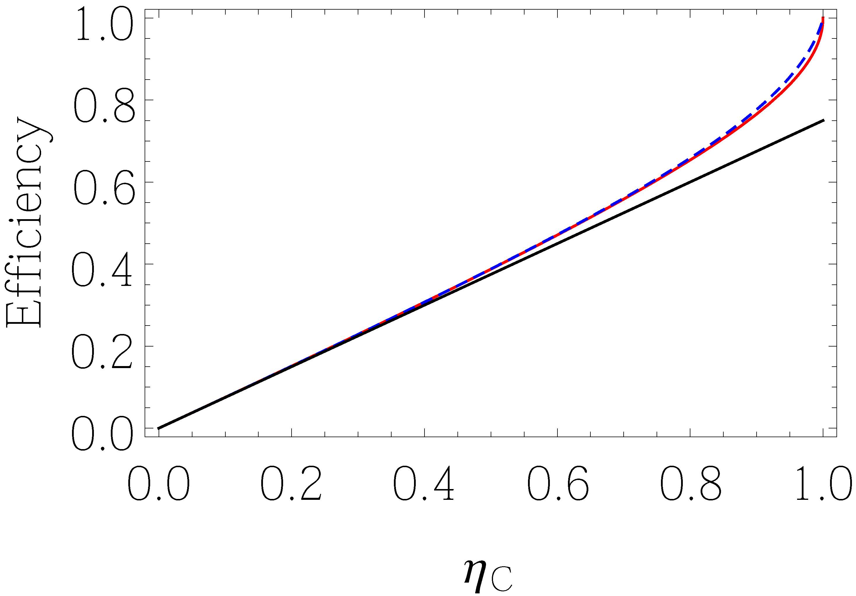
Figure 1.
The efficiency at maximum ecological function, obtained from two different methods, is plotted versus . The dashed curve represents the efficiency obtained from two-parameter optimization (Equation (16)). The solid curve is the corresponding efficiency when prior information approach is used (Equation (26)). The bottom straight line is . See also Equation (27).

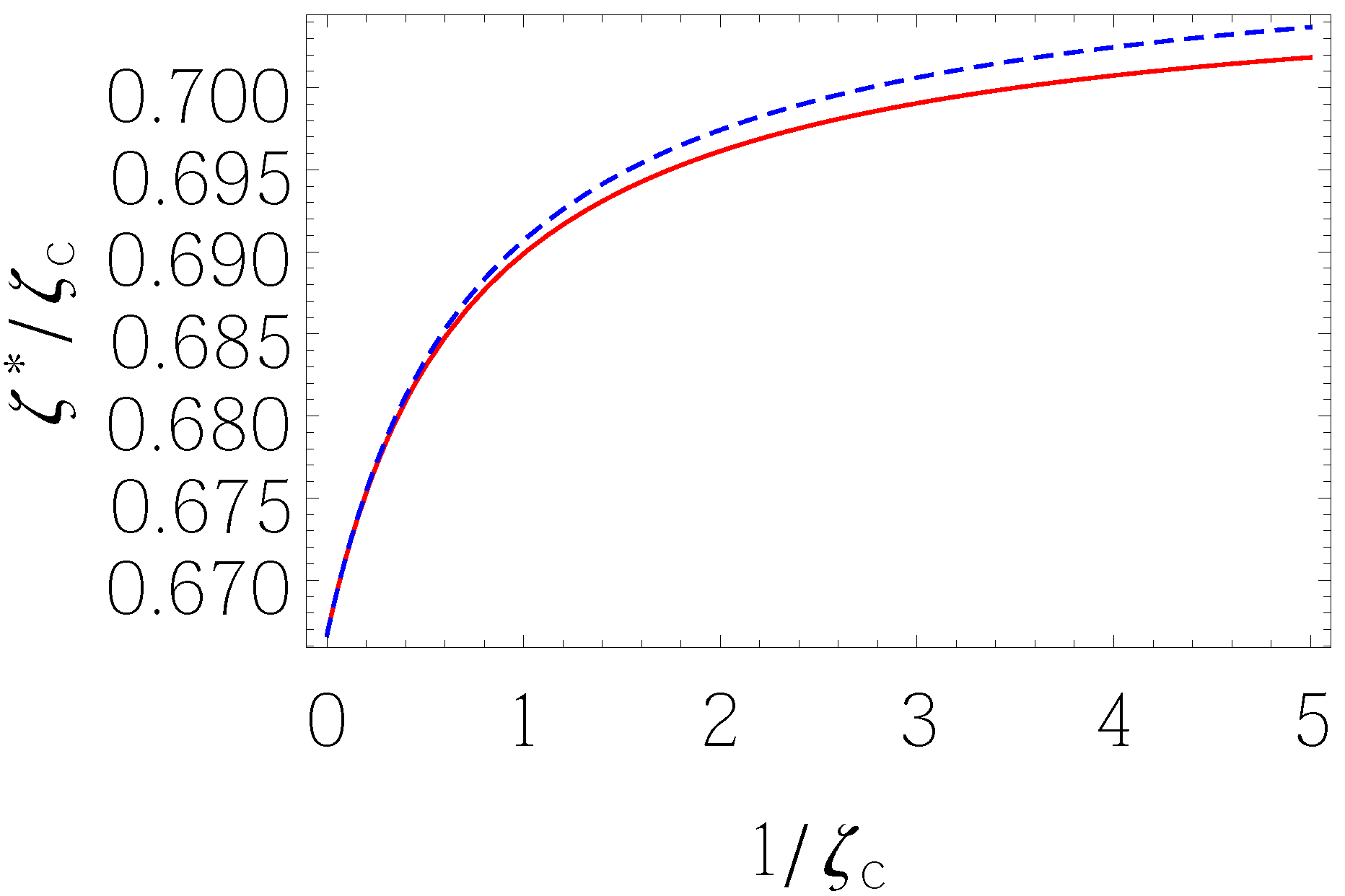
Figure 2.
The COP (relative to ) at maximum ecological function, obtained from two different methods, is plotted versus . The dashed curve represents the COP obtained from two-parameter optimization (Equation (37)). The solid curve is the corresponding COP when prior information approach is used (Equation (46)).

© 2017 by the authors. Licensee MDPI, Basel, Switzerland. This article is an open access article distributed under the terms and conditions of the Creative Commons Attribution (CC BY) license (http://creativecommons.org/licenses/by/4.0/).
Share and Cite
MDPI and ACS Style
Singh, V.; Johal, R.S. Feynman’s Ratchet and Pawl with Ecological Criterion: Optimal Performance versus Estimation with Prior Information. Entropy 2017, 19, 576. https://doi.org/10.3390/e19110576
AMA Style
Singh V, Johal RS. Feynman’s Ratchet and Pawl with Ecological Criterion: Optimal Performance versus Estimation with Prior Information. Entropy. 2017; 19(11):576. https://doi.org/10.3390/e19110576
Chicago/Turabian StyleSingh, Varinder, and Ramandeep S. Johal. 2017. "Feynman’s Ratchet and Pawl with Ecological Criterion: Optimal Performance versus Estimation with Prior Information" Entropy 19, no. 11: 576. https://doi.org/10.3390/e19110576
Note that from the first issue of 2016, this journal uses article numbers instead of page numbers. See further details here.