The Mean Field Theories of Magnetism and Turbulence

Abstract

In the last few decades a series of experiments have revealed that turbulence is a cooperative and critical phenomenon showing a continuous phase change with the critical Reynolds number at its onset. However, the applications of phase transition models, such as the Mean Field Theory (MFT), the Heisenberg model, the XY model, etc. to turbulence, have not been realized so far. Now, in this article, a successful analogy to magnetism is reported, and it is shown that a Mean Field Theory of Turbulence (MFTT) can be built that reveals new results. In analogy to compressibility in fluids and susceptibility in magnetic materials, the vorticibility (the authors of this article propose this new name in analogy to response functions, derived and given names in other fields) of a turbulent flowing fluid is revealed, which is identical to the relative turbulence intensity. By analogy to magnetism, in a natural manner, the Curie Law of Turbulence was discovered. It is clear that the MFTT is a theory describing equilibrium flow systems, whereas for a long time it is known that turbulence is a highly non-equilibrium phenomenon. Nonetheless, as a starting point for the development of thermodynamic models of turbulence, the presented MFTT is very useful to gain physical insight, just as Kraichnan’s turbulent energy spectra of 2-D and 3-D turbulence are, which were developed with equilibrium Boltzmann-Gibbs thermodynamics and only recently have been generalized and adapted to non-equilibrium and intermittent turbulent flow fields.

1. Introduction

Turbulence is an order-disorder phenomenon belonging to the field of statistical physics [1]. Ordinary people intuitively associate chaos and turbulence to be inherently linked with disorder. However, the scientific terminology is exactly the opposite. In this article, the smooth laminar flow defines the phase in a fluid being in disorder, but the more it is externally excited and becomes turbulent, by symmetry breaking, the more order appears. It will be shown that order in turbulent flows is defined by the fluctuation intensity or its turbulent kinetic energy. Therefore, the constant velocity of laminar flow (stress parameter) is not a result of symmetry breaking like the occurrence of a well-defined magnetization (order parameter) in a magnetic system is. As a result, we can say that a laminar flow, with the turbulence intensity as order parameter, shows full translational and rotational symmetries. Usually for large Reynolds number it is believed that a flow approaches homogeneous and isotropic turbulence, which is statistically without structure and therefore, would show the highest symmetry. However, microscopically this is not the case. If in a model consideration small vortices are assumed to occur in the infinite Reynolds number limit their number tends to infinity and their diameter to zero. Thus, to conclude that they disappear is a wrong inference. Finally, the result is that usually the creation of an ensemble of different structure scales, especially small ones, leads to much lower symmetries. On the other hand, in macroscopic models of turbulence (with a cut-off of e.g., high-wavenumber eddies) such assumptions are allowed to be made and, thereby, a virtual higher symmetry may be assumed that leads to simpler results in this limiting case. As a result of all these considerations, a corresponding generalized entropy (see e.g., [2]) for increasing Reynolds number decreases. An increasing stress of a fluid dynamic system is described by an increasing characteristic velocity of the physical system, or in a dimensionless number presentation, by an increasing overall Reynolds number, $R{e}_0$ [3]. Therefore, flows with the highest turbulence intensity are occurring when its Reynolds number is infinite. Order in such systems has to do with cooperative behavior, and it usually occurs when a critical value of the external stress is exceeded; in our case this is the critical overall Reynolds number $R{e}_{0_c}$.

Other physical systems showing cooperative or critical behavior are magnetic systems, where magnetic moments or spins align (you may think of the aligned hairs in a crew cut of a soldier), defining order in a very obvious manner. Disorder occurs here above a critical temperature, called the Curie temperature, T_c, and the order of the system increases if the temperature T is decreased below T_c, reaching its maximum at T = 0 K.

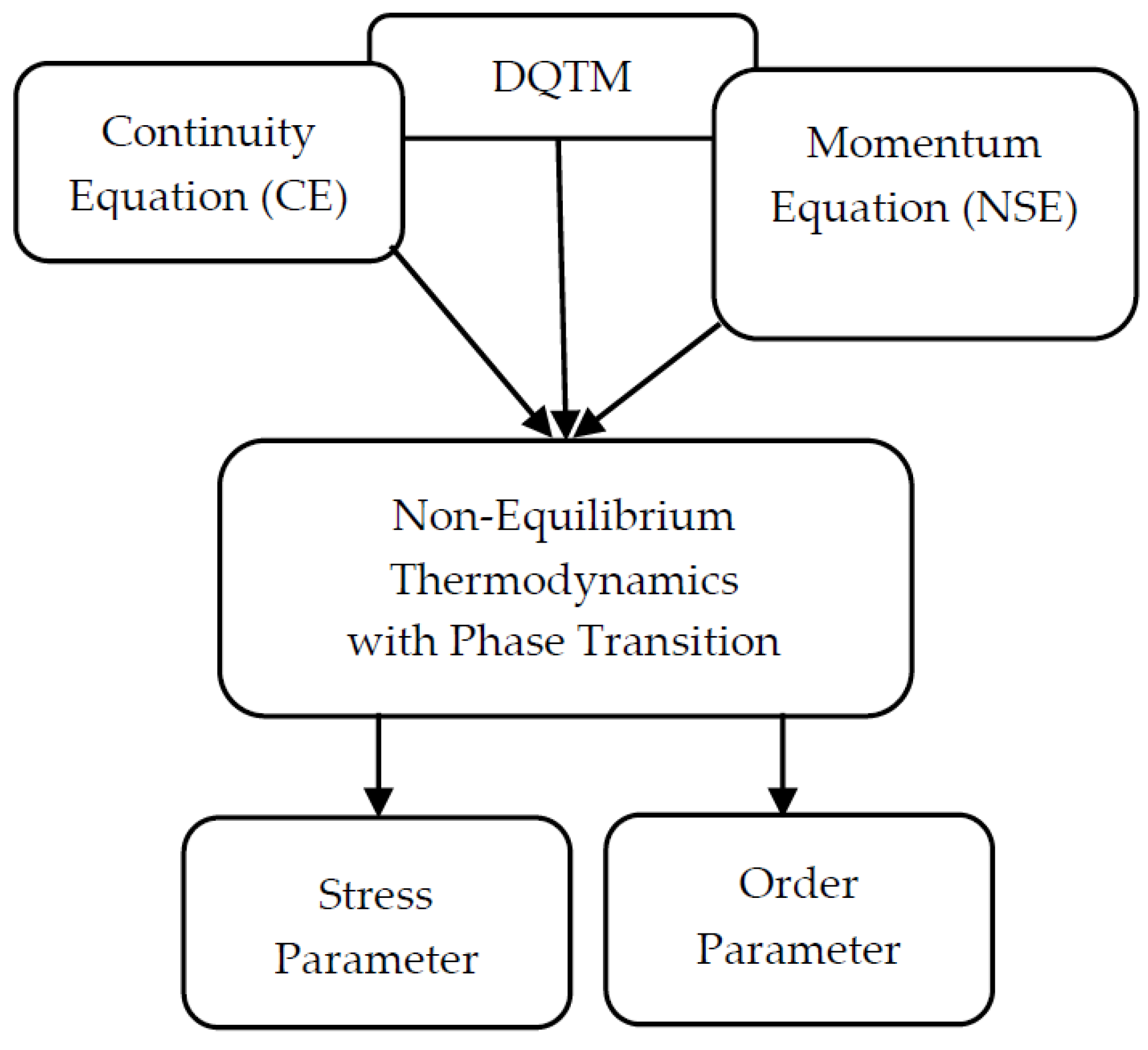
Egolf et al. solved analytically plane turbulent Couette [4], Poiseuille [5] and “wall” flows [6] by applying a nonlocal and fractional turbulence model [7,8], the Difference-Quotient Turbulence Model (DQTM) (see [9,10]). If the continuity and the Navier-Stokes equation (see [11]) are in a self-similar manner combined with the DQTM, in all these cases a critical phenomenon with a continuous phase transition is revealed (see Figure 1). Confirming statements of order-disorder in the work of Egolf et al. (see Refs. [4,5,6,10]), the stress parameter (for a definition see below) occurs inversely, namely as 1/$R{e}_0$. Thus, one may state that, in analogy to magnetism, the Reynolds number should have been defined inversely or that thermodynamics should be consequently performed by using as its stress parameter the coldness 1/T, instead of the temperature T.

It is beyond the scope of this article to review all the articles on turbulence, where the authors have discovered critical phenomena and the phase change character of turbulence. However, such a review of the authors of this article is found in [12]. Briefly, we may state that most of these articles are experimentally motivated (see e.g., [13,14]). The related fluid dynamic experiments show a criticality and the authors are aware that there is a turbulence quantity that serves as an order parameter. Cortet et al. [15] used time series of stroboscopic particle image velocimetry data to study the response of a von Kármán swirling flow between Re = 100 and 1,000,000. The flow can be characterized by a scalar, the modulus of the global angular momentum. Its response is linear with a slope depending on Re and shows a divergence at a critical Reynolds number. This divergence coincides with spontaneous symmetry breaking, whereas the statistics transforms from a Gaussian to a Non-Gaussian distribution with metastable and nonsymmetrical states. Time intermittencies between metastable states are observed. The authors write in their final sentence of their abstract: “We show that these observations can be interpreted in terms of divergence of the susceptibility to symmetry breaking, revealing the existence of a phase transition. An analogy with the ferromagnetic-paramagnetic transition in solid-state physics is presented.” More than thirty years ago, Pomeau [16] described the laminar-turbulent transition of a fluid by coupled oscillators. This was a kind of preliminary stage for a statistical description of this transition and paved the way for applications of percolation ideas performed by Alhoff and Eckhardt [17], Kreilos et al. [18], Lemoult et al. [19] and Wester et al. [14]. We further discuss results of the research division of the last listed authors. These scientists apply knowledge from percolation analysis in order to temporally and spatially resolve a boundary layer transition in a channel flow. The percolation theory allows them to describe a complex phase transition with only three critical exponents. Particle Image Velocimetry (PIV) experiments yield the basis for these investigations. In percolation theory, the data need to be binarized with the help of a threshold value, which in their case is the magnitude of the fluid velocity. In the percolation theory a cell is either laminar or turbulent. It is evident that this concept is in excellent agreement with the phase change concept of turbulent flows, where the fluid field is separated also into two states or phases, respectively, namely into laminar streaks and turbulent patches. Wester et al. validate critical exponents (see below) of the directed percolation theory by experimental means with good accuracy. Also other authors realized that there could exist an analogy to magnetic systems (e.g., [20,21]), and generalized temperatures were introduced as stress parameters of turbulent systems (e.g., [22,23]). Furthermore, many authors claimed about a lack of existence of clear theories and models, describing turbulent phase transitions [21,24]. This article presents a first attempt to improve this incompleteness in the field of turbulence. It hopefully leads to a standardization in the sense that stress and order parameters are not arbitrarily chosen, with definitions that vary from paper to paper.

This article has two main objectives. The first is to introduce the right analogy between magnetism and turbulence in the context of critical phenomena exhibiting continuous phase transitions. Having knowledge of magnetism, this analogy helps to better understand turbulence and vice versa. Secondly, with this analogy, it is possible to transform thermodynamic theories for magnetic systems to systems describing turbulent flows. In a first attempt this has now been performed for the simplest model, the Mean Field Theory (MFT). This procedure already reveals two main results. First, in analogy to the Curie law in magnetism, a new law-called Curie law of turbulence-was discovered. Second, strict mathematical derivations based on this law lead to the right response function and energy of turbulence. The authors take these results as a first validation of this new discovered law. A collection of other new laws, where some of them show a divergence at the critical Reynolds number (compare with experimental observations in Ref. [15]), are outlined, and this occurs again in analogy to corresponding formulas in magnetism.

It is likely that future and more sophisticated approaches will describe non-equilibrium systems of turbulence: They will be based on extended thermodynamics [2], involving Non-Gaussian statistics [25], anomalous diffusion [26], fractional calculus [27], etc. However, one has to be aware that Kraichnan [28] worked out e.g., valuable approximate 2-D and 3-D spectra of turbulence by applying equilibrium Gibbs-Boltzmann statistics. In the same sense, starting humbly, we will test, whether one of the oldest and simplest models of phase transitions, namely the MFT, which was very successfully applied, e.g., to paramagnetic-ferromagnetic phase transitions (see e.g., [29,30]), also applies to describe turbulence. By doing so, we were strongly guided by recently discovered perfect analogies between magnetic and turbulent systems, see [12].

2. Cooperative Phenomena

In this section we introduce the basic concepts of phase transitions in an ad hoc manner. A verification of these results and a presentation of a firmer basis, at least on the level of a macroscopic model, will follow in Section 3 and Section 4. One should be aware that models like the MFT are generally called ad hoc solution models (see e.g., [31]).

2.1. What Is a Critical or a Cooperative Phenomenon?

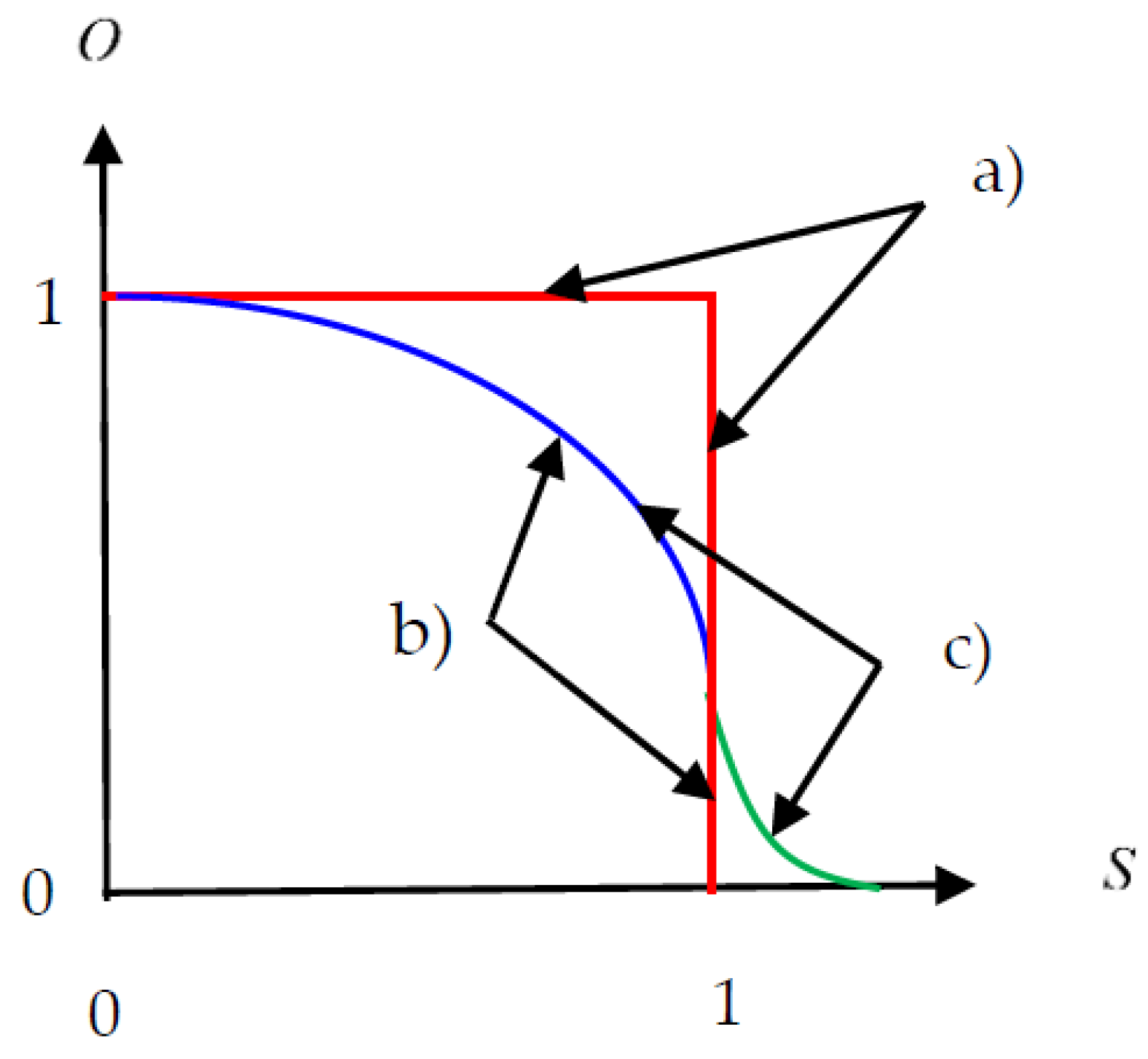
For readers, not so familiar with critical phenomena, we start our explanations with a solid-liquid phase transition. Lowering at constant pressure $p_0$ the temperature T of a sample of liquid, e.g., water, from above its critical temperature, T_c = T_W = 0 °C at normal pressure (1 atm = 101,325 Pa), below this critical value, leads to a sudden change from its liquid to its solid state. Each of the two phases is characterized by its own specific volume v, specific energy e, entropy s, etc. At criticality some of these quantities jump, or, as we say in a more mathematical manner, they are discontinuous. Therefore, such changes in the material state are called discontinuous phase transitions. These phase transitions are alternatively also called first-order phase transitions (see Figure 2a).

If we now add a certain percentage of a freezing suppressing additive, e.g., alcohol or glycol, to the water, then, by decreasing the temperature, the solid phase is continuously produced. The reason is that the freezing process is practically reduced to the water/ice transition. Therefore, in the shrinking water content the additive concentration rises and, thus, shifts the transition temperature of transforming water to ice continuously to lower temperatures. So, this process is a continuous phase transition (Figure 2b). The substance then transforms from the liquid to the solid region through a mushy two-phase region. Such melting-freezing processes are successfully modeled, e.g., by the Continuous-Properties Model (CPM) of Egolf and Manz [33]. In this approach melting and freezing are calculated by nonlinear diffusion. These authors showed that, like in solutions of the Burgers equation, the temperature profiles show a steepening effect. Egolf and Manz observed theoretically steepening of the profiles to the front or to the back and both. For water, the mushy substance is called ice slurry, a binary fluid that is applied in refrigeration technologies to transport efficiently the cold. Ice slurry may, for instance, be modeled as a Bingham fluid, which has higher flow resistance than pure water, but, because of the very high latent heat, is still energetically favorable for the transport of cold energy (see e.g., [34,35,36,37]).

Intriguing is that a variety of systems in different areas of scientific domains exhibit analogous critical phenomena. They are observed in fields where statistical physics applies, just as it is also the case in turbulence. Such systems are, as we have just discussed, liquid/solid transitions, but they also exist as gas/liquid transitions, magnetic systems with spontaneous magnetization in solid state probes with small internal magnetic field changes (see e.g., [29,30,38]), systems with spin-ordering in Ising ferromagnets or Ising antiferromagnets and spin glasses [32], ⁴He at the critical lambda-point [30], etc.

Another feature occurring in phase transitions is symmetry breaking. In liquid/solid transitions this phenomenon occurs, because a regular crystal microscopically has a higher symmetry than the irregularly located atoms or molecules in the liquid phase. On the other hand, a gas/liquid transition has no such change of symmetry and, therefore, also no symmetry breaking. An example of a magnetic system with symmetry breaking will also be given below.

2.2. Stress and Order Parameters

In a description of materials showing a phase change it is essential to identify the main external stress parameter of a system, which by division with its critical value, $s_c$, at which eventually symmetry breaking occurs, becomes dimensionless:

$$S=\frac{s}{s_c}\begin{array}{cc}& \end{array}\Rightarrow \begin{array}{cc}& \end{array}S\in (0,\infty ).$$

(1)

This parameter characterizes the external forcing of a system, and therefore, is also called control parameter. A non-equilibrium thermodynamic system is externally forced away from equilibrium. This led scientists of nonlinear dynamics to prefer the designation stress parameter, as its monotonic numerical amplification increases the stress on the system.

In a liquid/solid transition system the stress parameter is the temperature T or, alternatively, its coldness 1/T. Related to the imposed impact on a system, it reacts in its specific manner. Non-equilibrium systems can even spontaneously organize their internal structure and raise the order, which is a process that is today well known in many scientific areas and called self-organization process (see e.g., Haken [39,40]). It is initiated by instabilities and bifurcations, which are related to the critical stress parameters. The occurrence of a von Kármán eddy distribution behind a cylinder is an impressive example of such a process (see below). The internal organization and, simultaneously, the order of the system is described by an order parameter O. This parameter is generally set to zero above criticality; below this, for lower temperatures it is (monotonically) increasing toward “1”, indicating the route to highest order, and lowest entropy, respectively (see Figure 2b). It appears evident that such an order parameter curve O(S) essentially characterizes a physical system.

Let us now define the order parameter. With knowledge that can be acquired by studying Refs. [4,5,6,10], we set it in a very general manner as:

$$O=\frac{o-o_c}{o_p-o_c},\begin{array}{cc}& \end{array}\Rightarrow \begin{array}{cc}& \end{array}O\in \left[0,1\right],$$

(2)

where o denotes an appropriate changing property, which may be constant above criticality (Figure 2b), but not as displayed in Figure 2c, and increases monotonically below it toward smaller values of S. Furthermore, the quantity O is its dimensionless counterpart. The index c denotes here the critical and p a pole value, which indicate the properties of the lowest and the highest order phase, respectively. Often, the critical parameter o is so defined that its value at criticality is $o_c=0$ and Equation (2) simplifies to:

$$O=\frac{o}{o_p}.$$

(3)

Note that order parameters may be numerous mathematical objects as scalars, pseudo-scalars, vectors, tensors, elements of symmetry groups, etc. (see [30,32]).

Returning to the static fluid system, its density has the properties which an order parameter must possess, namely e.g., a monotonic increase of its value toward lower temperatures. Therefore, in agreement with Equation (2), we may write:

$$O=\frac{\rho -{\rho }_{\mathrm{liquid}}}{{\rho }_{\mathrm{solid}}-{\rho }_{\mathrm{liquid}}}\begin{array}{c}\\ \end{array}\Rightarrow \begin{array}{c}\\ \end{array}O\in \left[0,1\right].$$

(4)

In a model, it is often assumed that the pure liquid and solid phases show temperature-independent physical properties. Then, we have at and above criticality a pure liquid phase $\rho ={\rho }_{\mathrm{liquid}}$ and the order is at its lowest value (O = 0). On the other hand, at T = 0 K there exists only the pure solid phase $\rho ={\rho }_{\mathrm{solid}}$, and here the order is at its maximum (O = 1) (see Figure 2a).

Not all systems show homogenously dispersed mushy regions. However, it could be that ice blocks are floating in equilibrium with water, as it can be observed in the arctic sea. In such cases the property o (in the present case the density ρ) would have to be an integral measure, respectively a spatial average of the material containing domain.

The relation of the order parameter to the inherent order of the system can be easily explored in a paramagnetic-ferromagnetic phase transition (see Figure 3). In a paramagnetic sample, above a critical temperature, T_c, the approximately equal number of up and down spins of the system are randomly distributed. The order defined by the spins is characterized by their magnetization m. A spin up counts $s^{\uparrow }=+1$ (or + 1/2 in the case of an electronic spin) and a spin down $s^{\downarrow }=-1$ (or − 1/2), respectively. Therefore, above T_c, statistically the magnetization M is zero. It is defined by Equation (3):

$$M=\frac{m}{m_p}\cong \frac{\sum s^{\uparrow }+\sum s^{\downarrow }}{\sum s},\begin{array}{cc}& \end{array}\sum s=\sum s^{\uparrow }+\sum \left|s^{\downarrow }\right|$$

(5)

In the first Equation (5), we have assumed that the spins are very small and numerous, so that the magnetization M can be regarded as a continuous variable. Because we only consider spins in a predefined and its opposite direction, we have written the otherwise vectorial quantity “magnetization” as a scalar. When lowering the temperature T below the critical stress parameter $S_c=T_c,$ the spins begin to order and by this the magnetization increases. 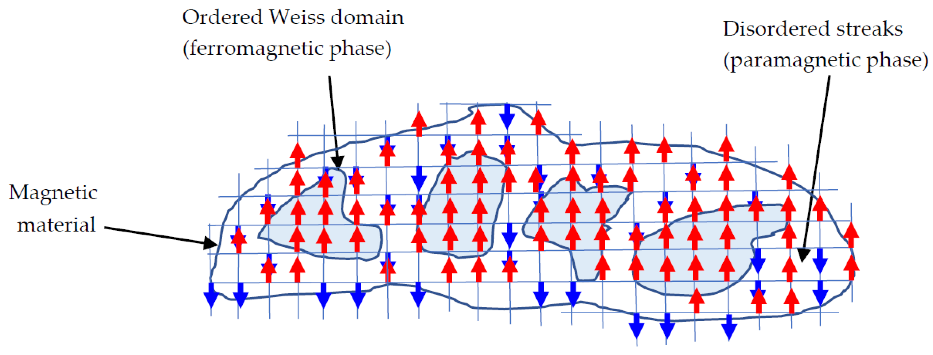If all spins are directed upward, their number is equal to the total sum of all absolute spin values, $\sum s$, and then the normalized magnetization M is equal to “1”. Therefore, the magnetization can serve as an ideal order parameter of this magnetic system. In magnetism, such orderings may occur in patches (islands of aligned magnetic moments), where complete order occurs, whereas in the remaining local areas the elementary magnets are still in a fully disordered state. In terms of phase transitions the disordered patches are one phase and the ordered ones define the second phase, called Weiss domains (Figure 3).

At criticality the spins are disordered. Decreasing the temperature birth is given to small Weiss domains, which, with lower temperature, occur more numerous and start to grow, till at T = 0 K the entire area is a single fully ordered Weiss-domain. This picture is analogous to the ice blocks in the arctic sea, and, also here one requires the introduction of an integral quantity as a suitable order parameter:

(6)

a global quantity, that is an effective magnetization, known as magnetic moment.

2.3. Symmetry Breaking

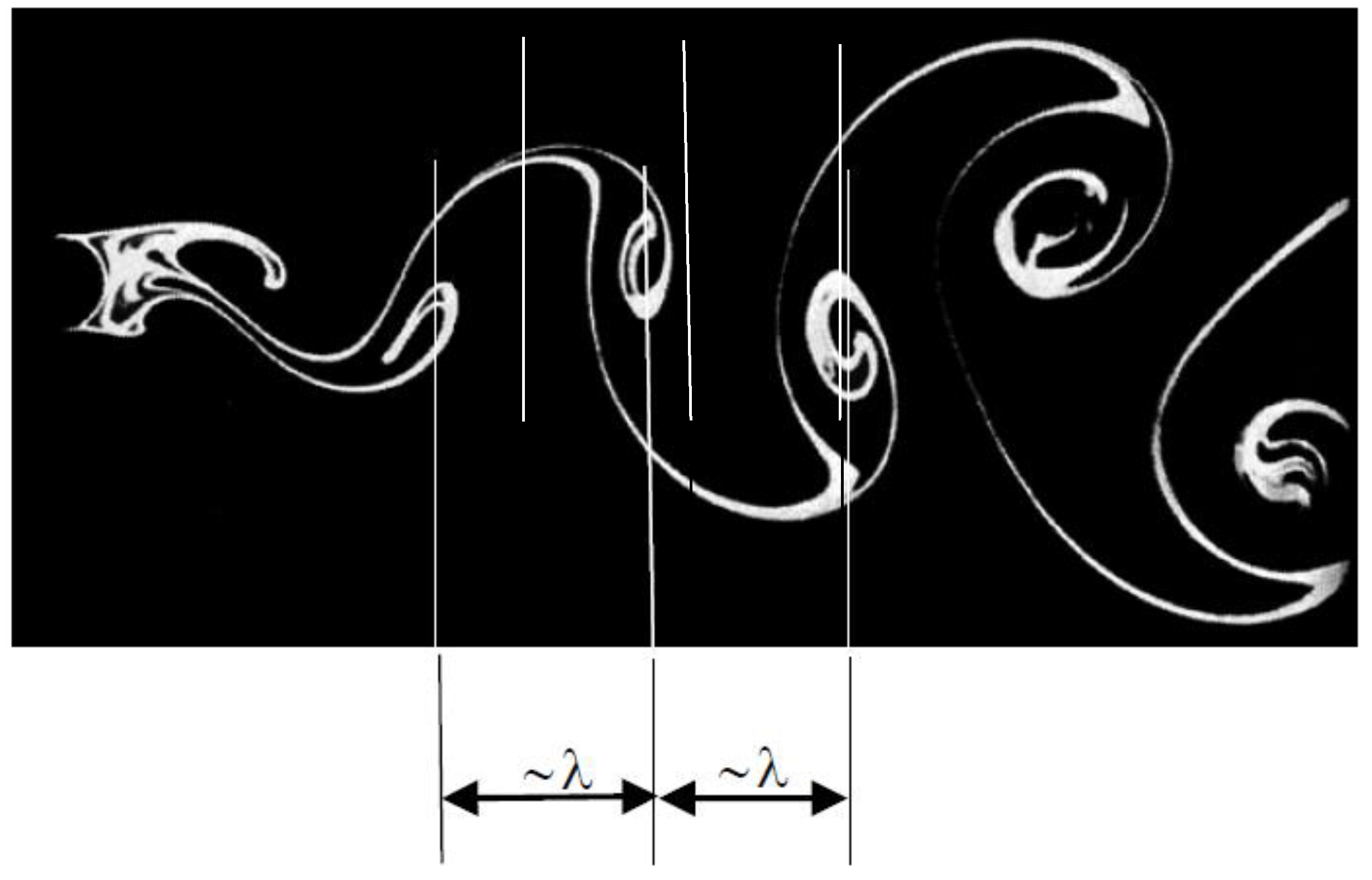
We already encountered two examples of physical systems showing symmetry breaking. The first is the von Kármán vortex street. Laminar flow in the downstream direction behind a cylinder has the highest symmetry; it is insensitive to all kinds of translations and rotations. On the other hand, by an increase of the stress parameter of the fluid dynamic system (this parameter being the overall Reynolds number $R{e}_0$) above its threshold value $R{e}_{0_c}$, it creates spatially periodic structures (see Figure 4). These limit the translational variance to distances of periodic length λ. Such a restriction is called symmetry breaking and is related to a decrease of the (generalized) entropy (see e.g., Refs. [2,41]). At this point a subtlety must be explained. In the simple thermodynamic modeling of this article the first instability defines the critical point and that’s it! This is the bifurcation point where steady behaviour transforms to temporal behaviour. In the MFT of a von Kármán flow behind a cylinder, it is also the critical Reynolds number where periodic von Kármán eddies appear. These structures are not turbulent; only after a further increase of the overall Reynolds number a transition to quasi-periodic structures, chaos, soft and strong turbulence occurs. Different fluid dynamic systems show different scenarios of transitions to turbulence (see e.g., Refs. [39,40]). It is beyond scope of this article to discuss these different types of transitions. This lack is also justified, because the MFT, presented in this article, does not describe the transitions in all its details. An important subtlety is that our model describes the transition from laminar to pulsating or fluctuating behaviour, including at slightly higher Reynolds number also the turbulent states; more precisely it is not a direct transition from laminar to turbulent flow.

The second example is the magnetic physical system just discussed above. The stress parameter is the temperature, which by a decrease below its critical value, the Curie temperature Τ_c , initiates an ordering of spins. By this the homogeneity is lost and the system, in a natural manner, creates a preferential direction. Rotational symmetry is then only preserved around the axis pointing in this direction. By alignments of elementary magnetic moments, respectively spins, the energy of the system decreases to become a minimum at zero absolute temperature. The disordered phase, occurring in the interval $T_c$ ≤ T ≤ ∞, is called paramagnetic phase and the phase with some order, observed between 0 ≤ T < $T_c$, is denoted ferromagnetic phase. In a magnetic system, the alignment of magnetic moments is also remarkably influenced by a second stress parameter, namely the internal magnetic field H.

2.4. Response Functions and Crtical Exponents

Now let us assume that there are two stress parameters $s_1$ and $s_2$ of a system and a single order parameter O(s₁,s₂). Following Equation (2), we study the dependence of O on $s_1$ by setting $s_2=0$:

$$O\left(s_1,0\right)=f\left(\frac{s_1-s_{1c}}{s_{1p}-s_{1c}}\right),\begin{array}{cc}& \end{array}{s}_1\le s_{1c},$$

(7)

where the exact form of the function f is sought. For criticality, we request (see Figure 2b):

$$f\left(s_{1c}\right)=f(0)=0,$$

(8)

and for the pole value:

$$f\left(s_{1p}\right)=f(1)=1.$$

(9)

A power law with a positive (possibly fractional) exponent β′ fulfills these two requirements (references with tables and quantitative values are given below)

$$O\left(s_1,0\right)={\left(\frac{s_1-s_{1c}}{s_{1p}-s_{1c}}\right)}^{\beta \prime }.$$

(10)

If $O\left(s_{1c},0\right)\ne 0$ then we redefine the order parameter as the difference $\Delta O=O\left(s_1,0\right)-O\left(s_{1c},0\right)$. This is the case for the liquid-solid transition, but not for the magnetic transition, discussed, as we will see.

Such a power law description may/may not be approximate when applied to the entire domain [0, 1] of O, however close to criticality, it yields a fairly accurate formula. Therefore, from now on we mainly will apply this equation only in the limit as criticality is approached and define:

$$\beta \prime =\underset{\epsilon \to 0}{\lim }\frac{{\log }_{e}O\left(\epsilon \right)}{{\log }_e\epsilon },\begin{array}{cc}& \end{array}\epsilon =\frac{s_1-s_{1c}}{s_{1p}-s_{1c}},\begin{array}{cc}& \end{array}{s}_1\le s_{1c}.$$

(11)

The exponent β′ is called critical exponent. Finally, the order parameter is recalled to be:

$$O\left(s_1,0\right)={\left(\frac{s_1-s_{1c}}{s_{1p}-s_{1c}}\right)}^{\beta \prime }, s_1\le s_{1c}, \beta \prime >0.$$

(12)

For consistency reasons, we denote this exponent by β′ just as the denotation in the main literature (see e.g., [29,30,31,32]). In Figure 2 it is seen that we can choose $s_{1p}=0$, transforming Equation (12) to the following formula:

$$O\left(s_1,0\right)\propto {\left(1-\frac{s_1}{s_{1c}}\right)}^{\beta \prime },\begin{array}{c}\\ \end{array}{s}_1\le s_{1c},\begin{array}{c}\\ \end{array}\beta \prime >0.$$

(13)

Next, the order parameter O will be studied as a function of the second stress parameter $s_2$ at criticality $s_{2c}$ at fixed $s_1=s_{1c}$, which is along an isoline:

$$O\left(s_{1c},s_2\right)\propto {\left(\frac{s_2-s_{2c}}{s_{2c}}\right)}^{1/\delta },\begin{array}{cc}& \end{array}\delta >0,$$

(14)

and in which the critical exponent is written for reasons of tradition as the constant 1/δ. The reaction of the property of the bulk material and of the order parameter o to a change of the stress parameter $s_2$ at constant $s_1$ can be estimated by the quantity:

$${\psi :=\frac{\partial O}{\partial s_2}|}_{s_1}.$$

(15)

Assume that $O\left(s_1,0\right)$ describes the order parameter with a form as shown in Figure 2c. Then, scaling, given by a power law, is present on both sides of the critical point $s_{1c}$. Now, one may write, e.g., for the exponent γ′ if $s_1<s_{1c}$ and γ if $s_1>s_{1c}$. The quantity Ψ is discontinuous at criticality, as is clearly seen from

$$\psi \propto \{\begin{array}{c}{\left(1-\frac{s_1}{s_{1c}}\right)}^{-\gamma \prime },\begin{array}{c}\\ \end{array}{s}_1<s_{1c},\begin{array}{c}\\ \end{array}\gamma \prime >0,\\ {\left(\frac{s_1}{s_{1c}}-1\right)}^{-\gamma },\begin{array}{c}\\ \end{array}{s}_1>s_{1c},\begin{array}{c}\\ \end{array}\gamma >0.\end{array}$$

(16)

The related critical exponents are usually identical; i.e., γ′ = γ (see e.g., [29]). These two-fold values occur for most critical exponents as discussed below. However, because of brevity, in the following sections we always merely formulate a single version (16). The negative sign in the exponents of (16) is introduced to have positive values for γ and γ′. A further advantage is that a negative sign visibly signalizes that this physical quantity diverges as criticality is approached. A further quantity that diverges as $s_{1c}$ is approached may exist; it is described by:

$$\phi \propto {\left(1-\frac{s_1}{s_{1c}}\right)}^{-\alpha \prime },\begin{array}{cc}& \end{array}{s}_1\le s_{1c},\begin{array}{cc}& \end{array}\alpha \prime >0,$$

(17)

with the critical exponent α′.

The special case of a liquid-solid transition is obtained by identifying the first stress parameter with the temperature, $s_1=T$, and the second with $s_2=p_c$. The order parameter was already introduced to be the density ρ of the fluid. With these identities Equation (13) becomes:

$$\Delta \rho =\rho \left(T,p_c\right)-\rho \left(T_c,p_c\right)\propto {\left(1-\frac{T}{T_c}\right)}^{\beta \prime },\begin{array}{cc}& \end{array}\beta \prime >0.$$

(18)

Correspondingly, Equation (14) transforms to:

$$\Delta \rho =\rho \left(T_c,p\right)-\rho \left(T_c,p_c\right)\propto {\left(\frac{p-p_c}{p_c}\right)}^{1/\delta },\begin{array}{cc}& \end{array}\delta >0.$$

(19)

Let us, next, describe the reaction of a static fluid system, subjected to a change of its order parameter (being the volume O = V) by an altering pressure field $s_2=p$ at constant temperature $s_1=T$. It is given by Equation (15), which is adapted to the symbols of the physical properties of a static fluid, and where the negative sign guarantees a positive value of the compressibility, viz.:

$${{\kappa }_T=-\frac{1}{V}\frac{\partial V}{\partial p}|}_T.$$

(20)

${\kappa }_T$ is the compressibility at constant temperature and must be distinguished from the adiabatic compressibility at constant entropy ${\kappa }_S$. If the volume change, caused by a unit of pressure change, is large, the system is said to be highly compressible, and if this quantity is zero, the fluid is incompressible. Following Equations (16), the compressibility diverges toward criticality from below (exponent γ’) and above (exponent γ). Then, for example, the low temperature case is described by the formula:

$${\kappa }_T\propto {\left(1-\frac{T}{T_c}\right)}^{-\gamma \prime },\begin{array}{cc}& \end{array}T\le T_c,\begin{array}{cc}& \end{array}\gamma \prime >0.$$

(21)

Another diverging quantity of the type of Equation (17) of a fluid system is the specific heat at constant volume, $C_V$, characterized by the critical exponent α′:

$$C_V\propto {\left(1-\frac{T}{T_c}\right)}^{-\alpha \prime },\begin{array}{cc}& \end{array}T\le T_c,\begin{array}{cc}& \end{array}\alpha \prime >0,$$

(22)

which must be distinguished from the specific heat at constant pressure, $C_p$.

In analogy to the liquid-solid transitions, the special case of a magnetic system is obtained by substituting for the first stress parameter the temperature, $s_1=T$, and for the second one, the external magnetic field $s_2=H_0$. The dimensionless order parameter was already introduced to be the magnetization M. Thus, Equation (13) becomes:

$$M\left(T,0\right)\propto {\left(1-\frac{T}{T_c}\right)}^{\beta \prime },\begin{array}{cc}& \end{array}T\le T_c,\begin{array}{cc}& \end{array}\beta \prime >0.$$

(23)

Furthermore, Equation (14) transforms to the following order parameter/stress parameter relation:

$$M\left(T_c,H_0\right)\propto {\left(H_0-H_{0_c}\right)}^{1/\delta }=H_0{}^{1/\delta },\begin{array}{cc}& \end{array}\delta >0,$$

(24)

where $H_{0_c}=0$ is usually suppressed. Next, consider the reaction of a magnetic system, described by a change of its order parameter (the magnetization O = M) to an altering magnetic field $s_2=H_0$, at constant temperature $s_1=T$. It is given by Equation (15), which is adapted to the magnetic symbols; this yields:

$${{\chi }_T=\frac{\partial M}{\partial H_0}|}_T.$$

(25)

This derivative of M with respect to $H_0$ at fixed T is called the differential magnetic susceptibility at constant temperature and is denoted by ${\chi }_T$. Just as it was the case for the compressibility, also the susceptibility diverges as criticality is approached (from below and above). The first (low temperature) case is described by the formula:

$$\chi \propto {\left(1-\frac{T}{T_c}\right)}^{-\gamma \prime },\begin{array}{cc}& \end{array}T\le T_c,\begin{array}{cc}& \end{array}\gamma \prime >0.$$

(26)

In a magnetic system, its ability to react to opposed stress is quantified by its susceptibility χ. If the magnetization change is large, caused by a unit of magnetic field change, the system is said to be easily magnetizable, and if this quantity is zero, the magnetic material is non-magnetizable. Quantities, such as the compressibility of a fluid and the susceptibility of a magnetic system, are called analogous response functions.

Furthermore, following Equation (17), another diverging quantity of a paramagnetic to ferromagnetic phase transition system is the specific heat at constant magnetic field, $C_{H_0}$ (in strict analogy, it would have to be $C_M$, the specific heat at constant magnetization M, instead of $C_{H_0}$, the specific heat at constant external magnetic field $H_0$), which is characterized by its exponent α′:

$$C_{H_0}\propto {\left(1-\frac{T}{T_c}\right)}^{-\alpha \prime },\begin{array}{cc}& \end{array}T\le T_c,\begin{array}{cc}& \end{array}\alpha \prime >0.$$

(27)

These thermomagnetic quantities are reviewed by Egolf et al. (see in Refs. [43,44]). The interested reader must have recognized that there is a perfect analogy between the discussed fluid and magnetic systems. The corresponding quantities are shown in

Table 1. Analogy between a static fluid phase transition and a magnetic phase transition. Recall that the specific volume v is related to the density of the fluid ρ by v = 1/ρ.

Quantity	Fluid	Magnet
Stress parameter 1	T	T
Stress parameter 2	p	$H_0$
Order parameter	v (ρ)	M
Specific heat	$C_V$	$C_M$
Response function	${\kappa }_T$	${\chi }_T$

.

In the discussion of the most important critical exponents two additional quantities defining such are important, namely the pair correlation and the correlation length.

2.5. Pair Correlation Function and Correlation Length

To derive the pair correlation, let us study the particle number density $n(\overrightarrow{r})$ of a physical system with N particles (in this paragraph we follow the presentation in Ref. [31]):

$$n(\overrightarrow{r})=\sum _{k=1}^N\delta \left(\overrightarrow{r}-{\overrightarrow{r}}_k\right).$$

(28)

Defining $\langle \left(\dots \right)\rangle$ as the ensemble average of $\left(\dots \right)$, its second-order correlation function:

$${\varsigma }_2=\langle n(\overrightarrow{r})n(\overrightarrow{r}\prime )\rangle ,$$

(29)

is proportional to the conditional probability of meeting a particle at position $\overrightarrow{r}$ if there is another particle at position $\overrightarrow{r}\prime$. Closely related to this quantity is the pair or density-density correlation function

$$G\left(\overrightarrow{r},\overrightarrow{r}\prime \right)=\langle \left[n(\overrightarrow{r})-\langle n(\overrightarrow{r})\rangle \right]\cdot \left[n(\overrightarrow{r}\prime )-\langle n(\overrightarrow{r}\prime )\rangle \right]\rangle ,$$

(30)

which is a measure of the correlations of the fluctuations of the particle density.

In the special case that a system is spatially uniform (translationally invariant), it follows that:

$$G\left(\overrightarrow{r},\overrightarrow{r}\prime \right)=G\left(\overrightarrow{r}-\overrightarrow{r}\prime \right).$$

(31)

Employing the denotation:

$$n\equiv \langle n(\overrightarrow{r})\rangle =\langle n(\overrightarrow{r}\prime )\rangle ,$$

(32)

Equations (30) and (32) can be combined to yield

$$\begin{array}{l}G\left(\overrightarrow{r}-\overrightarrow{r}\prime \right)=\langle \left[n(\overrightarrow{r})-n\right]\cdot \left[n(\overrightarrow{r}\prime )-n\right]\rangle =\langle \left[n(\overrightarrow{r})n(\overrightarrow{r}\prime )-n n(\overrightarrow{r})-n n(\overrightarrow{r}\prime )+n^2\right]\rangle \\ =\langle n(\overrightarrow{r})n(\overrightarrow{r}\prime )\rangle -2n \langle n(\overrightarrow{r})\rangle +n^2.\end{array}$$

(33)

Applying again (32), yields:

$$G\left(\overrightarrow{r}-\overrightarrow{r}\prime \right)=\langle n(\overrightarrow{r})n(\overrightarrow{r}\prime )\rangle -n^2.$$

(34)

For $\left|\overrightarrow{r}-\overrightarrow{r}\prime \right|\to \infty$ we can assume that the probability of finding a particle at position $\overrightarrow{r}\prime$ is independent of the presence of a particle at $\overrightarrow{r}$. However, if the densities are uncorrelated, it follows that:

$$\langle n(\overrightarrow{r})n(\overrightarrow{r}\prime )\rangle =\langle n(\overrightarrow{r})\rangle \langle n(\overrightarrow{r}\prime )\rangle =n^2.$$

(35)

Hence, Equation (34) shows that, in the limit of large distances, the pair correlation function G vanishes:

$$G\left(\overrightarrow{r}-\overrightarrow{r}\prime \right)\to 0, \left|\overrightarrow{r}-\overrightarrow{r}\prime \right|\to \infty .$$

(36)

In linear and in thermal equilibrium systems, this behavior is often described by an exponential decay at $T_c$ and $p_c$ (see e.g., Refs. [32,45]):

$$G\left(r\right)\propto \frac{1}{r^{d-2+\eta }}\exp \left(-\frac{r}{\xi }\right),$$

(37)

with η being the critical exponent of the pair correlation function G. In this formula d denotes the Euclidean dimension of the system and ξ is the correlation length of the density fluctuations. It is a measure giving the distance over which cooperative behavior is perceptible and corresponds to characteristic sizes of the already discussed patches, e.g., Weiss domains. Toward criticality the correlation length scales also with a power law:

$$\xi \propto {\left(1-\frac{T}{T_c}\right)}^{-\nu \prime }, T\le T_c, \nu \prime >0,$$

(38)

and diverges with the critical exponent v′.

Stanley [31] demonstrates by a clear and brief calculus, using the Boltzmann factor of a grand canonical ensemble, that:

$$\frac{{\kappa }_T}{{\kappa }_{T,0}}=\frac{1}{n}\underset{\mathrm{\Gamma }}{\int }G\left(\overrightarrow{r}\right)dV,$$

(39)

where ${\kappa }_{T,0}$ is the isothermal compressibility of an ideal gas. This law is the analogue to the fluctuation-dissipation theorem of a static fluid. It proves that an increase (divergence) of the compressibility is related to an increase of the density fluctuations and to the range of the density-density correlation function.

2.6. Universality: Yes or No?

We have now introduced the main critical exponents α′, β′, δ, γ′, η and ν′ and the counterparts α and γ, of which some experimentally determined values are listed in

Table 2. Quantities of critical exponents given by models and experiments for a selection of different physical systems for the range $T<T_c$. Data taken from Ma [29] and Stanley [31].

Quantity	α′	β′	δ	γ′	ν′
Fluids	---	---	---	---	---
CO2	~0.1	0.34	4.2	~1.0	-
Xe	<0.2	0.35	4.4	~1.2	0.57
Magnets	---	---		---	---
Ni	−0.3	0.42	4.22	1.32	-
EuS	−0.15	0.33	-	-	-
CrBr3	-	0.368	4.3	-	-
Models	---	---		---	---
Classical	0	1/2	3	1	1/2
Spherical 3-D	-	1/2	5	-	-
Ising 2-D	0	1/8	~15	~7/4	1
Ising 3-D	~1/8	~5/16	~5	~5/4	-
Heisenberg 3-D	-	~0.35	~5	-	-

. Why is in the literature and in this section so much attention given to the limit toward criticality, respectively to critical exponents, if the complete functions contain much more information? The answer is that experimentally it was observed that different systems, to a very high experimental accuracy, show the same values. This can be seen, for example in Table 2, where the critical exponents of the order parameter of the fluids CO₂ and Xe are 0.34 and 0.35, respectively. Many more such fluids show these values (see e.g., [29,30]). Yet, not only this, also the magnetic system, e.g., composed by EuS, shows a critical exponent β′ = 0.33. Furthermore, for example, the 3-D Heisenberg model (see e.g., [46,47]) predicts a value exactly in this range. Therefore, some decades ago, scientists were convinced that critical exponents are a manifestation of a kind of universal behavior of systems showing phase transitions. For example, in the three-dimensional Ising antiferromagnetic material ${\mathrm{DyAlO}}_3$, the exponent β′ was, for $T\to T_c$ (from below), experimentally determined to be β′ = 0.311 ± 0.005. Goldenfeld [32] writes that the observed values of β′ for a liquid-solid transition and a para-ferromagnetic phase transition system, within the accuracy of the performed experiments, were determined to be the same. So, early researchers believed that the critical exponents of all order parameter curves were 1/3. However, Ho and Lister [48] (see also e.g., in Ref. [31]) demonstrated unequivocally that for the insulating ${\mathrm{CBr}}_3$ material β′ = 0.368 ± 0.005 (see Table 2), disproving such an assumption.

Even if such deviations and imperfections are generally accepted today, in the scientific community the consensus is that toward criticality, where correlation and long-range order measures increase, the nature of the short-range interactions may become less significant. This explains that systems in different areas of physics reveal so similar or even identical critical laws.

Basic interaction models, as e.g., listed in Table 2, reveal equations and inequalities that relate the different critical exponents to each other. These dependencies yield the possibility that if e.g., two critical exponents are known that a third critical exponent can be calculated. In Table 2 one can find the critical exponents for static fluids and magnetic systems and the theorectical values given by different magnetic interaction models. The classical values correspond to the values derived with the MFT (see also Section 3 and Section 4). The spherical model is also a simple model to describe ferromagnetism. It was solved in 1952 by Berlin and Kay [49]. It is a model that can be analytically solved in the presence of an external field. The Ising model [46] was formulated by Lenz in 1920 and solved by his student Ising. It describes magnetic dipole moments also as next neighbour entities in a regular lattice configuration. The one-dimensional Ising model does not show a phase transition, whereas the higher-dimensional Ising models do. The Heisenberg model [47] is more sophisticated than the models discussed above and serves for the study of critical behaviour and phase transitions of quantum mechanical systems. One finds more information on all these models and their derivations in Refs. [29,30,31,32]. If a complete description of critical exponents is envisaged, the above mentioned relations between the critical exponents are very important. However, because our investigations on phase transitions in turbulence are still in its infancy, we at present do not already have need for them. For the interested reader, who wants to explore more on this topic, an excellent survey is given by Stanley [31].

In this review, by discussing later the MFT, we only touch the surface of standard and well-accepted theories on phase transitions, including the theoretical discoveries made possible by the application of the DQTM to solve elementary turbulent shear flows. Our intention is to highlight and explore analogies occurring between turbulent flows and other physical systems known for decades to reveal phase transitions. So now, we will switch shortly from the liquid and magnetic model systems back to turbulence.

2.7. A Turbulent Phase Transition with Its Two Phases

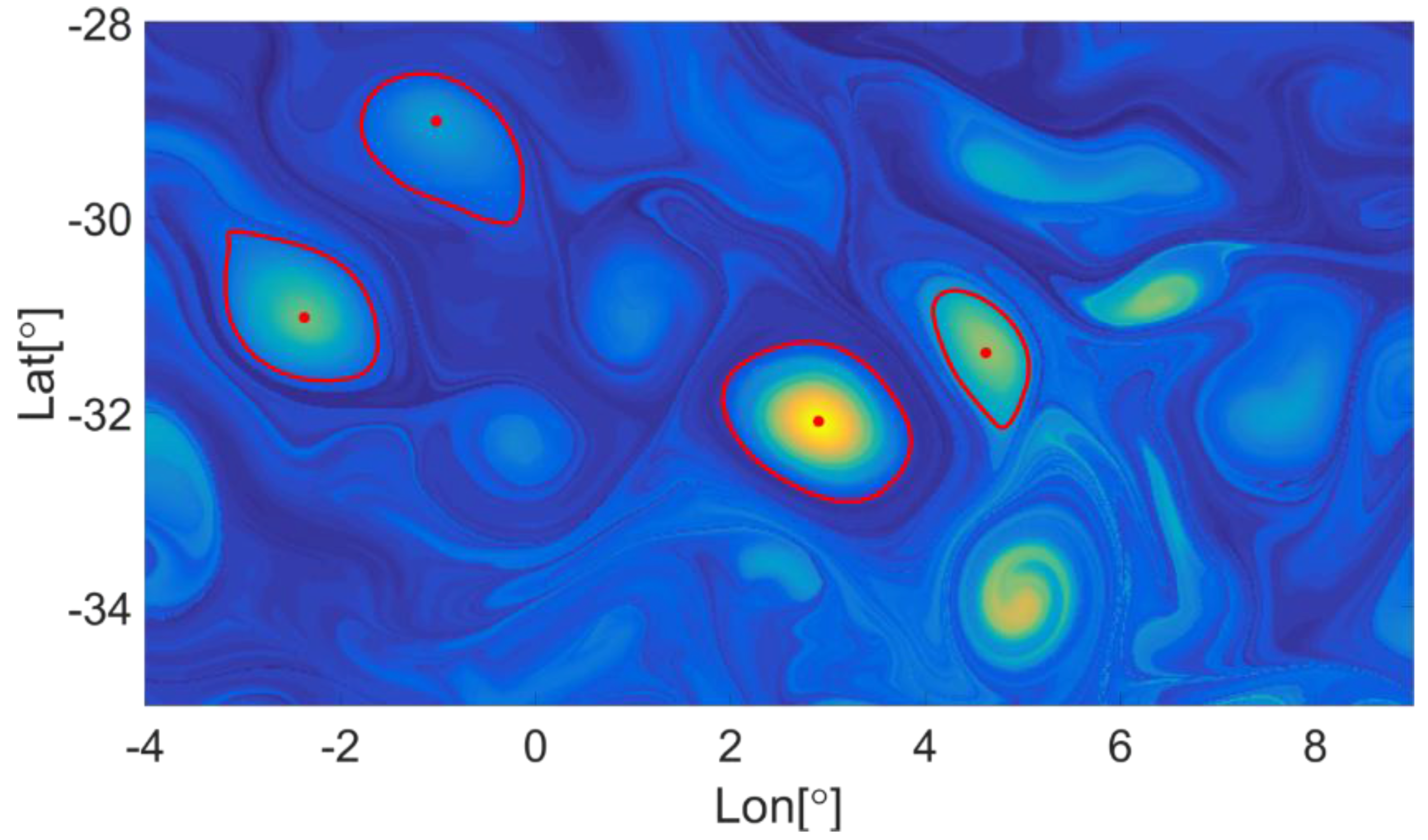
If turbulence is stated to be a cooperative or critical phenomenon exhibiting phase transitions, the first question that arises is the question what the two phases are and what makes their difference. By thinking in analogies this question can be easily answered. In a liquid system, the low order phase is the pure liquid and the high-order phase is the pure solid phase. In turbulence, the lowest-order phase, with the highest symmetry properties, is laminar flow and the highest-order phase, in this case, would be an infinite Reynolds number turbulent flow. Therefore, e.g., in a medium Reynolds number flow, we should be able to distinguish subdomains of calm laminar streaks from regions of high turbulent activity, showing a high production rate of kinetic fluctuation energy, of vorticity and enstrophy, etc. This picture fits very well with Leonardo da Vinci’s view, demonstrated in numerous drawings of turbulent water flows. In a description Leonardo even wrote: “Observe the motion of the surface of the water, …, which has two motions, …, one part of which is due to the principal current, the other to the random and reverse motion” [50]. It is intriguing how his observations support the two-phase picture of turbulence, which is strongly advertised in this review article! Therefore, we summarize that coherent structures are separated from rather inactive flow regions. Furthermore, we claim that the vorticity-rich regions are low-entropy regions, and we classify them to be the analogous patterns, called Weiss domains in magnetic phase transition systems. Today the study of coherent structures is a main activity in turbulence research, where some part of the studies is experimental and the larger part is performed by direct numerical simulations (DNS). Because of reasons of length, it is beyond the scope to review this research domain in this article. However, a concise review of the authors on laminar streaks and coherent structures is found in Ref. [12]. To give some impression of the two distinct patterns, Figure 5 is presented. One can distinguish dark blue lengthy regions that represent the laminar streaks. In these regions there is no whirling motion. On the other hand, approximately circular regions stand for the vorticity rich domains. The most intense whirling areas are marked by red circular surrounding lines.

3. Mean Field Theory of a Paramagnetic to Ferromagnetic Phase Transition

We start with an old, but very successful model of phase transitions, namely the MFT and introduce it by following mainly arguments of Ma [29]. The method to advance is to review its simplest introduction for a ferromagnetic-paramagnetic phase transition, and then, in the next section, in analogy to apply it to turbulence.

Let us assume that a ferromagnetic body is brought into an external magnetic field $H_0$. An electron in the solid material is in a local internal magnetic field H, that is given by the external magnetic field $H_0$ plus an average magnetic or magnetization field, m, that originates from neighboring spins, which have the same direction as or the opposite one from the external field. Thus, the following theory is again written only in scalar variables. In the MFT, it is assumed that this additional field is a function of the average of all spins. Therefore, its value may slightly deviate from the actual magnetization that is strictly fulfilling the relation:

$$H=H_0+M.$$

(40)

For small m’s, we may assume that the external field is linear in this averaged magnetization:

$$H=H_0+a m,$$

(41)

with the relation:

$$M\cong a m\cong m,$$

(42)

assuming a value of the constant a close to “1”. The quantity m follows the Curie law, i.e.,:

$$m=c\frac{H}{T},$$

(43)

where c is another constant. By solving for m and eliminating the internal field H, in a combination of Equations (41) and (43), it follows that:

$$m=\frac{c{H}_0}{T-ac}.$$

(44)

The product ac must be a characteristic temperature of the problem. The only choice is the critical temperature:

$$T_c=ac.$$

(45)

Then, Equation (44) takes its final form:

$$m=\frac{c{H}_0}{T-T_c}, T>T_c.$$

(46)

Next, with the assumption in Equation (42), the differential susceptibility can be derived from (46) to yield:

$${\chi }_T\cong {\frac{\partial M}{\partial H_0}|}_T=\frac{c}{T-T_c}, T>T_c.$$

(47)

If the temperature converges towards the critical temperature, the magnetization and the susceptibility diverge, the latter with exponent γ = 1. These results are in agreement with experiments (see e.g., [29]).

This most simple approach delivers good results above criticality; however, it fails below the Curie temperature $T_c$.

To obtain reasonable results for the full domain, one must develop approximation (41) to a higher order:

$$H=H_0+a m+b m^3+O\left(m^5\right),$$

(48)

where the uneven power laws guarantee that the oppositely directed spins (e.g., those positioned in the downward direction) will contribute negatively to the internal magnetic field H. In this equation b is a negative constant. Now, combining Equations (43) and (48), it follows that:

$$bc m^3+ac m-Tm+c{H}_0=0.$$

(49)

Equation (45) remains valid and changes (49) to:

$$bc m^3+\left(T_c-T\right)m+c{H}_0=0.$$

(50)

Because the quadratic term is missing in the polynomial function of degree three, this is a reduced cubic equation of m that can be analytically solved either by the casus cardani or the casus irreducibilis method, depending on the numerical values of the constants. Here, it is sufficient to study only some special cases, as outlined below.

Firstly, we look at a domain of vanishing external magnetic field $H_0=0$ and temperatures below criticality, $T<T_c$. Then from Equation (50), it follows (apart from the trivial solution m = 0) a quadratic equation with the solution:

$$m\left(T,0\right)={\left[\frac{T-T_c}{bc}\right]}^{1/2}, T<T_c, b<0, c>0,$$

(51)

which is only meaningful for b < 0 (sic!). Moreover, by applying (42) and a comparison with Equation (23), the critical exponent is extracted to be:

$$\beta \prime =\frac{1}{2}.$$

(52)

To derive the susceptibility, the easiest way is to differentiate Equation (50) with respect to $H_0$ at constant temperature T:

$$3bc m^2{\frac{\partial m}{\partial H_0}|}_T+\left(T_c-T\right){\frac{\partial m}{\partial H_0}|}_T+c=0, T<T_c, b<0, c>0,$$

(53)

With Equations (42) and (47) this is identical to:

$$\left[3bc m^2+\left(T_c-T\right)\right]{\chi }_T+c=0, T<T_c, b<0, c>0.$$

(54)

Now, Equation (51) is inserted for m and Equation (54) is solved for ${\chi }_T$, which leads to:

$${\chi }_T=\frac{c}{2}\frac{1}{\left(T_c-T\right)}, T<T_c, c>0.$$

(55)

Comparing this equation with (26) yields a next critical exponent, namely:

$$\gamma \prime =1.$$

(56)

Secondly, we study the behavior of the magnetic system at the critical temperature, $T=T_c$. In this case, Equation (50) simplifies to:

$$b{m}^3+H_0=0, T=T_c, b<0,$$

(57)

revealing, in the following formula, a further critical exponent:

$$m\left(T_c,H_0\right)={\left(-\frac{H_0}{b}\right)}^{1/3}, b<0,$$

(58)

alerting us again that the constant b must be negative. Comparison with Equations (24) and (42) leads to:

$$\delta =3.$$

(59)

Thirdly, we look at the domain of vanishing external magnetic field $H_0=0$ and temperatures above criticality, $T>T_c$. For this region, the results are practically the same as for $T<T_c$, and we obtain:

$$m\left(T,0\right)={\left(\frac{T-T_c}{bc}\right)}^{1/2}, H_0=0, T>T_c, b>0, c>0.$$

(60)

where b is now positive. We conclude that:

$$\beta \prime =\beta =\frac{1}{2}.$$

(61)

As in the first case, but with $T-T_c$ instead of $T_c-T_{}$, the susceptibility is derived to be in analogy to (55):

$${\chi }_T=\frac{c}{2}\frac{1}{\left(T-T_c\right)}, T>T_c, c>0,$$

(62)

resulting in the equivalence of the critical exponents of these quantities:

$$\gamma \prime =\gamma =1.$$

(63)

With the approximation (42), the magnetic energy for a material with linear magnetization can be estimated by the formulas (see e.g., by Kitanovski and Egolf [43]):

$$E=-{\mu }_0{\mu }_{r }HM\cong -{\mu }_0{\mu }_{r }Hm.$$

(64)

The constant ${\mu }_0=4\pi \cdot {10}^{-7}{\mathrm{NA}}^{-2}$ denotes the magnetic permeability and ${\mu }_r$ the dimensionless relative magnetic permeability. We will only study the case of a vanishing external magnetic field $H_0=0$.

In the first case for ferromagnetic materials at temperatures below criticality, $T<T_c$, with Equation (41), it follows that:

$$E\cong -{\mu }_0{\mu }_{\mathrm{r}}\left(H_0+a m\right)m\cong -{\mu }_0{\mu }_{\mathrm{r}} m^2.$$

(65)

In this case the external magnetic field is zero, however the internal magnetic field, due to spontaneous magnetization, may be non-zero. Inserting Equations (51) into (65), it follows that:

$$E\cong -\frac{{\mu }_0{\mu }_{\mathrm{r}}}{bc}\left(T-T_c\right), H_0=0, T<T_c.$$

(66)

Furthermore, the specific heat $C_{H_0}$, at constant magnetic field $H_0$, is defined by the derivative:

$$C_{H_0}={\frac{\partial E}{\partial T}|}_{H_0}, H_0=0,$$

(67)

which with Equation (66) leads to:

$$C_{H_0}\cong -\frac{{\mu }_0{\mu }_{\mathrm{r}}}{bc}, H_0=0, T<T_c,$$

(68)

a specific heat that is positive, because b has a negative sign. Comparison with Equation (27) delivers a next critical exponent, namely:

$$\alpha \prime =0.$$

(69)

The second case, where the magnetic system is exactly at its critical temperature, $T=T_c$, reveals a discontinuity in the specific heat. This is shown by proving that the specific heat above the criticality is also constant (see third case), but shows a different value from that below criticality (see Equation (68)). Thus, with the help of the third case below, it will be proven that the specific heat shows discontinuous behavior.

In the third case at temperatures above criticality, $T>T_c$, there is no spontaneous magnetization, and it follows that:

$$E\equiv 0, T>T_c.$$

(70)

This implies that:

$$C_{H_0}\equiv 0, T>T_c$$

(71)

and:

$$\alpha =\alpha \prime =0, T>T_c.$$

(72)

Comparing (68) and (71), it is evident that the specific heat is discontinuous at criticality.

Summarizing, in the simplest manner, we have developed the MFT for a ferromagnetic-paramagnetic phase transition and have derived some classical critical exponents shown in Table 2 (bold values). They are also called mean field exponents. Ma [29] writes: “They do not agree very well with the [measured] values. However, in view of how little we put in, the theory is remarkably successful. It shows that the field provided by neighboring spins is responsible for generating a nonzero magnetization below $T_c$”. In Table 2 the reader may compare the red classical critical exponents with the corresponding measured values and notice that they correspond (however some only very approximately). The theory also predicts a divergent susceptibility and exponents that are independent of any details. Because the ideas of the MFT, in strict analogy, can be applied to antiferromagnetic materials, liquid-gas binary alloys, and other critical systems, it is tempting to assume that the models in these alternative fields must reveal the same critical exponents. This led to the idea of the earlier formulated universality.

In the following sections our objective is to test whether the classical and successful MFT, up-to-present mainly applied in magnetism, could have an application to turbulence and might deliver new insights and eventually even new physical results. We will experience that this is indeed the case. Therefore, the next section is more than a review, because in that section primarily new results are presented. This is also the reason why this work has the heading “article”, even if it is more likely a review with numerous new results.

4. Mean Field Theory of Turbulence

Notice that in this section the MFT is developed for turbulence in an analogous manner to magnetism, described in Section 3. Therefore, for better comparison, it may be valuable to have a

Table 3. Analogous quantities of magnetism (second column) and turbulence (third column).

Stress Parameter $S_1$	Temperature T	Inverse characteristic velocity $1/u_0$
Stress parameter $S_2$	External magnetic field $H_0$	Absolute mean velocity $\left|\overline{u}\right|$
Hermaphrodite parameter	Internal magnetic field H	Absolute velocity $\left|u\right|$
Order parameter O	Magnetization M	RMS fluctuation quantity $\sqrt{\overline{u{\prime }^2}}$
Response function	Isothermal susceptibility ${\chi }_T$	Vorticibility at const. charact. velocity ${\tau }_{u_0}$
Energy	Magnetization energy E	Kinetic fluctuation energy E
Specific thermal capacity	Specific heat at constant external magnetic field $C_{H_0}$	Specific heat at constant absolute mean velocity field $C_{\left|\overline{u}\right|}$

in front, and in a case of doubts or a lack of understanding to check the analogous model derivations in Section 3, which are slightly more extensive than those in this chapter.

Following Egolf and Weiss’s [4] discovery that a generalized temperature, T, of plane Couette flow is inverse to the overall Reynolds number ${Re}_0$, that is proportional to the characteristic velocity $u_0$, we assume that the following analogy between magnetism and turbulence holds:

$$S_1=T \leftrightarrow S_1=1/u_0.$$

(73)

This and further analogies are listed in Table 3. Furthermore, we remark that an external magnetic field $H_0$ may be a constant or slowly varying field and the up and down flipping spins, leading to the magnetization M, have the character of a fluctuating quantity. Therefore, we propose the analogy of the basic (scalar) relation of magnetism with the decomposed first velocity component u of a fluid:

$$H=H_0+M \leftrightarrow u=\overline{u}+u\prime ,$$

(74)

which is composed of the one-dimensional mean velocity, $\overline{u}$, and fluctuation velocity component, $u\prime$. Furthermore, as second stress parameter (in a positive form), we assume that:

$$S_2=H_0 \leftrightarrow S_2=\left|\overline{u}\right|,$$

(75)

and the positive order parameter in the analogous formulation is proposed to be the rms fluctuation velocity:

$$O=M \leftrightarrow O=\sqrt{\overline{u{\prime }^2}}.$$

(76)

One could introduce, for example, the quantity $\left|\left|u\right|-{\left|u\right|}_c\right|$ as order parameter, a quantity that is zero or positive and Galilean invariant. However, the fact that it is not identical to zero in the entire laminar domain is a strong argument against such a choice. Such argumentation also annihilates other similar postulations.

Next, we assert that fluctuations are favorably initiated in neighborhoods of already fluctuating domains. More specifically, in analogy to magnetism, where an averaging is performed only over neighboring spins, here an averaging of fluctuations is also performed only over neighbouring cells. This does not seem to be an unrealistic assumption. Furthermore, a next neighbour approximation of the fluctuation quantity by an averaging only over neighbouring domains is required (which we assume without a concrete definition) with a linear dependence:

$$u=\overline{u}+a\upsilon \prime , \overline{\upsilon \prime }=0,$$

(77)

assuming here the value of a to be also close to “1”, so that $\upsilon \prime \approx u\prime$. There is a small, however important difference between a magnetic and a fluid dynamic system. Above criticality the magnetic system has always a magnetization given by its spins. However, in the statistical mean it may disappear. This is different in the fluid dynamic system, where above criticality there are never any fluctuations present. Notice, that in the MFT it is only important that above criticality toward higher values of the stress parameter the order parameter (which is an averaged quantity) decreases.

Now, by comparing (74) with (77), we write in analogy to (42):

$$\sqrt{\overline{u{\prime }^2}}\cong a\sqrt{\overline{\upsilon {\prime }^2}}\cong \sqrt{\overline{\upsilon {\prime }^2}}.$$

(78)

Next, we conjecture (again in analogy to magnetism, with its Curie law: $M=cH/T$) that a fluid dynamic system also follows such a law, which we call Curie law of turbulence:

$$\sqrt{\overline{\upsilon {\prime }^2}}=c{u}_0\left|\left|u\right|-{\left|u\right|}_c\right|.$$

(79)

In magnetism one has $H_{0_c}$ = 0 and in turbulence ${\left|\overline{u}\right|}_c\ne 0$. Therefore, the generalization of introducing the critical value in the turbulence case extends the applicability of the model without leading to any difficulties.

The correctness of the law (79) is not so easy to recognize. However, let us be pragmatic and see whether eventually ensuing results will come out to be more evident and, thereby, could give support to the validity of this new formula.

Imposing a linear approximation of Equation (80) (see below), different from that in magnetism, we experience that in modeling turbulence the theory fails below as well as above criticality. The reason is the strict absence of fluctuations above criticality.

Therefore, here we immediately introduce an approximation up to third order in the approximate rms-fluctuation velocity and, for consistency reasons, also introduce the critical value of the absolute flow velocity, ${\left|\overline{u}\right|}_c$. This quantity is obtained by adjusting the fluid dynamic system at the overall critical Reynolds number and by measuring a velocity component at the field location of interest, averaging it and then finally applying the operation “absolute value”. This yields:

$$\left|\left|u\right|-{\left|u\right|}_c\right|=\left|\overline{u}\right|-{\left|\overline{u}\right|}_c+a\sqrt{\overline{\upsilon {\prime }^2}}+b{\sqrt{\overline{\upsilon {\prime }^2}}}^3+O\left({\sqrt{\overline{\upsilon {\prime }^2}}}^5\right),$$

(80)

with coefficients a and b analogous to those in Equation (48). Combining Equations (79) and (80), eliminating $\left|\overline{u}\right|-{\left|\overline{u}\right|}_c$ and setting $ac=1/u_{0_c}$, in analogy to (50) yields:

$$bc{\sqrt{\overline{\upsilon {\prime }^2}}}^3+\left(\frac{1}{u_{0_c}}-\frac{1}{u_0}\right)\sqrt{\overline{\upsilon {\prime }^2}}+c\left|\left|\overline{u}\right|-{\left|\overline{u}\right|}_c\right|=0.$$

(81)

We could obtain analytical solutions of (81) for the three roots and then construct inferences for these. However, for the moment it is sufficient to solve some simple special cases.

Unfortunately, without a driving field $\left|\left|\overline{u}\right|-{\left|\overline{u}\right|}_c\right|$, no spontaneously created turbulent fluctua-tions exist. However, we may study a case, not by demanding that $\left|\left|\overline{u}\right|-{\left|\overline{u}\right|}_c\right|=0$, but instead e.g.,:

$$\sqrt{\overline{\upsilon {\prime }^2}} \gg c\frac{\left|\left|\overline{u}\right|-{\left|\overline{u}\right|}_c\right|}{\left(\frac{1}{u_{0_c}}-\frac{1}{u_0}\right)}\hspace{1em}\hspace{1em}\mathrm{and}\hspace{1em}\hspace{1em}\sqrt{\overline{\upsilon {\prime }^2}} \gg {\left(\frac{\left|\left|\overline{u}\right|-{\left|\overline{u}\right|}_c\right|}{\left|b\right|}\right)}^{1/3}$$

(82)

(Equations (82)–(84), (89), (94) and (97) are mainly restricted to a special case describing superfluidity). This is the case when the fluctuations are very large and the driving mean velocity field small. It is not expected that such realizations are often occurring in a usual fluid of a geophysical or technical flow with a Reynolds number above criticality (except in special flow realizations, as e.g., a fluid in a container with vibrating walls). On the other hand, it might find some applications in a superfluid that shows vanishing viscosity (see e.g., [52,53,54]). What we assume here is a superfluid applied as a fluid with practically negligible viscosity and no internal entropy (wave) generation. This is a model prototype of a low-viscosity fluid.

Under the above restrictions, the last term in Equation (81) may be neglected, so that:

$$bc{\left(\sqrt{\overline{\upsilon {\prime }^2}}\right)}^2+\left(\frac{1}{u_{0_c}}-\frac{1}{u_0}\right)=0, u_0>u_{0_c}, b<0, c>0.$$

(83)

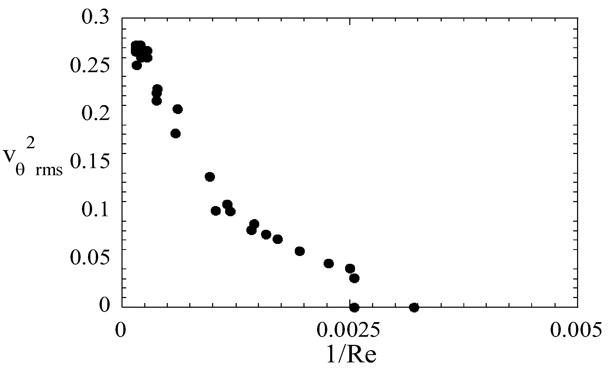
Solving for the full and approximate root mean square (rms) fluctuation intensity leads us to the results:

$$\sqrt{\overline{u{\prime }^2}}\cong \sqrt{\overline{\upsilon {\prime }^2}}={\left[\frac{1}{bc}\left(\frac{1}{u_0}-\frac{1}{u_{0_c}}\right)\right]}^{1/2}, u_0>u_{0_c}, b<0, c>0,$$

(84)

which are e.g., in analogy to Equation (51), leading again to the critical exponent β′ = 1/2.

Also in analogy to Equation (50), here we differentiate (81), with respect to $\left|\overline{u}\right|$ at constant inverse characteristic velocity $1/u_0$, to obtain:

$$3bc{\sqrt{\overline{\upsilon {\prime }^2}}}^2{\frac{\partial \sqrt{\overline{\upsilon {\prime }^2}}}{\partial \left|\overline{u}\right|}|}_{u_0}+\left(\frac{1}{u_{0_c}}-\frac{1}{u_0}\right){\frac{\partial \sqrt{\overline{\upsilon {\prime }^2}}}{\partial \left|\overline{u}\right|}|}_{u_0}+c=0. u_0>u_{0_c}. b<0, c>0.$$

(85)

In analogy to Equation (47), we introduce the differential response function of turbulence:

$${\tau }_{u_0}={{\frac{\partial \sqrt{\overline{u{\prime }^2}}}{\partial \left|\overline{u}\right|}|}_{u_0}\cong \frac{\partial \sqrt{\overline{\upsilon {\prime }^2}}}{\partial \left|\overline{u}\right|}|}_{u_0},$$

(86)

which we call “vorticibility”, which in a linearization is identical to the turbulence intensity and, for isotropic turbulence, also to the turbuence degree:

$${\tau }_{u_0}={\frac{\sqrt{\overline{u{\prime }^2}}}{\left|\overline{u}\right|}|}_{u_0}.$$

(87)

The differential vorticibility is substituted into Equation (85) and in analogy to (54) yields to:

$$\left[3bc{\sqrt{\overline{\upsilon {\prime }^2}}}^2+\left(\frac{1}{u_{0_c}}-\frac{1}{u_0}\right)\right]{\tau }_{u_0}+c=0, u_0>u_{0_c}, b<0, c>0.$$

(88)

Now, Equation (84) is inserted for $\sqrt{\overline{\upsilon {\prime }^2}}$ to yield, in an analogy to Equation (55), the following result:

$${\tau }_{u_0}=\frac{c}{2}\frac{1}{\left(\frac{1}{u_{0_c}}-\frac{1}{u_0}\right)}, u_0>u_{0_c}, c>0,$$

(89)

which allows identification of the critical exponent $\gamma \prime =1$.

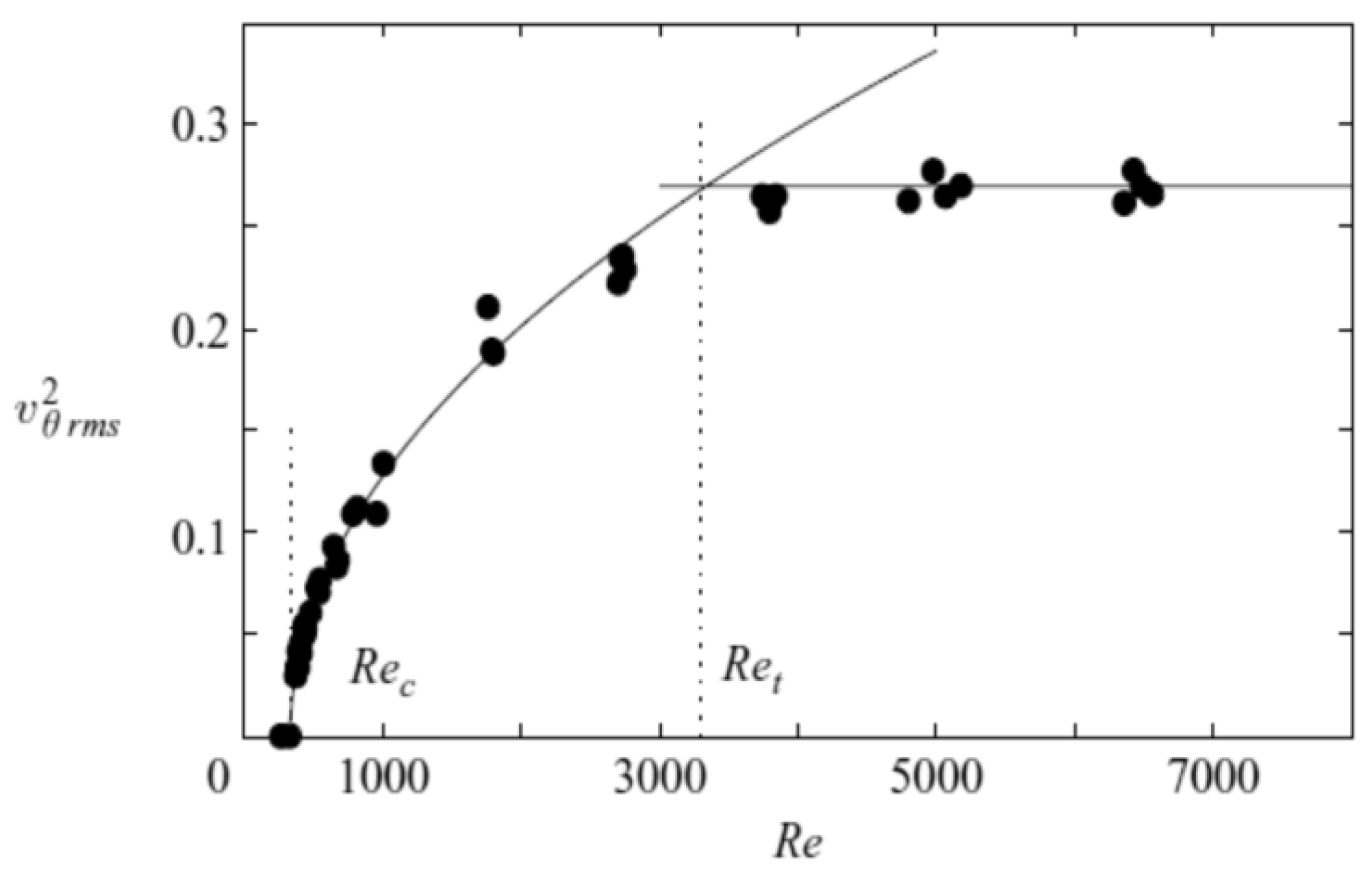
The vorticibility is the response function of a turbulent flow. The higher the increase of the turbulence intensity is, that is created by an increase of a unit of the absolute mean velocity, the larger will be the response of the turbulent system. A fluid with zero vorticibility is not able to produce per se any instabilities and fluctuations and in analogy corresponds to an incompressible fluid or non-magnetizable material. In a superfluid the vorticibility as a function of the inverse characteristic velocity approaches criticality from below with a divergence, described by a power law with critical exponent γ′ = 1.

More generally valid is the description of the turbulent system just at the inverse critical characteristic velocity $1/u_{0_c}$. Then, Equation (81) simplifies to:

$$b{\sqrt{\overline{\upsilon {\prime }^2}}}^3+\left|\left|\overline{u}\right|-{\left|\overline{u}\right|}_c\right|=0, \mathrm{at} u=u_{0_c},$$

(90)

revealing a further critical exponent:

$$\sqrt{\overline{u{\prime }^2}}\left(\frac{1}{u_{0_c}},\left|\left|\overline{u}\right|-{\left|\overline{u}\right|}_c\right|\right)\cong -{\left(\frac{\left|\left|\overline{u}\right|-{\left|\overline{u}\right|}_c\right|}{b}\right)}^{1/3}, \mathrm{at} u=u_{0_c}, b<0.$$

(91)

The fluctuation intensity at constant (critical) inverse characteristic velocity varies as a function of the absolute mean fluid velocity difference $\left|\left|\overline{u}\right|-{\left|\overline{u}\right|}_c\right|$ by a power law with the critical exponent 1/δ, where δ = 3, see [29].

The energy of the turbulent system is also the product of a stress and an order parameter, which in analogy to magnetism, where $E=-{\mu }_r{\mu }_{0}HM$, is given by:

$$E=d\left|\left|u\right|-{\left|u\right|}_c\right|\sqrt{\overline{u{\prime }^2}}\cong d\left|\left|u\right|-{\left|u\right|}_c\right|\sqrt{\overline{\upsilon {\prime }^2}},$$

(92)

with a constant d > 0 that will be later identified. We simply concentrate on the part describing the turbulent kinetic energy. Then, by inserting the linear term in $\sqrt{\overline{\upsilon {\prime }^2}}$ of Equation (80) and setting a = 1, it follows that:

$$E\cong \frac{\rho }{2}\overline{\upsilon {\prime }^2}\cong \frac{\rho }{2}\overline{u{\prime }^2},$$

(93)

where Equation (78) was applied, and the constant was identified to be d = ρ/2. We notice that the energy term of magnetism, in its analogy to turbulence, leads to the correct expression. However, it is rightly the positive turbulent kinetic energy of the flow, which is here presented in a one-dimensional approach. A generalization to the three-dimensional form is straightforward. Finally, the analogy between magnetism and turbulence is different by the sign in their energies. Whereas a magnetic system lowers its energy in a cooling process from zero to negative values with its minmum at the absolute zero point, a turbulent system also shows zero turbulent intensity at criticality, but with decreasing inverse overall Reynolds number, it shows an increasing turbulence intensity. This is taken into consideration by setting different signs in Equations (64), (92) and (93).

Next, the restricted form (84) is substituted into (93), which yields:

$$E\cong \frac{\rho }{2bc}\left(\frac{1}{u_0}-\frac{1}{u_{0_c}}\right), u_0>u_{0_c}, b<0, c>0.$$

(94)

This equation shows that at the critical point the turbulent kinetic energy is zero. Because above criticality, in a domain called the laminar regime, no fluctuations are present, one finds that:

$$E\equiv 0, u_0<u_{0_c}.$$

(95)

The specific heat $C_{\left|\overline{u}\right|}$ at constant mean velocity $\left|\overline{u}\right|$ is:

$$C_{\left|\overline{u}\right|}={\frac{\partial E}{\partial \left(\frac{1}{u_0}\right)}|}_{\left|\overline{u}\right|}.$$

(96)

For the domain below criticality, it follows with Equations (94) and (96) that:

$$C_{\left|\overline{u}\right|}=\frac{\rho }{2bc}<0, \mathrm{since} b<0.$$

(97)

In classical equilibrium thermodynamics a condition of stability requires $C_{\left|\overline{u}\right|}$ to be positive, when regarded as a function of the Reynolds number. However, here we have the inverse Reynolds number as independent variable. Therefore, when $C_{\left|\overline{u}\right|}\equiv C_{\left|\overline{u}\right|}\left(1/\mathrm{Re}\right)=C_{\left|\overline{u}\right|}\left(\mathrm{Re}\right)d\left(1/\mathrm{Re})\right)/d\mathrm{Re}=-1/{\mathrm{Re}}^2{C}_{\left|\overline{u}\right|}\left(\mathrm{Re}\right)$, which demonstrates that, in the present 1/Re-dependence of $C_{\left|\overline{u}\right|}$, the sign of $C_{\left|\overline{u}\right|}$ changes and, thus, in this notation stability prevails if Equation (97) is valid.

The “specific heat” of turbulence in a superfluid is the turbulent kinetic energy introduced to the turbulent flow field occurring by an increase of the stress parameter of the system, which is the characteristic velocity or overall Reynolds number.

In the domain above criticality one observes no fluctuations and, therefore, $E\equiv 0$ everywhere. Then, from Equation (96), it follows that:

$$C_{\left|\overline{u}\right|}\equiv 0.$$

(98)

Comparing the specific heat below criticality (see Equation (97) and above (Equation (98)), one recognizes that:

The specific heat of a turbulent superfluid at the critical Reynolds number is discontinuous. The critical exponents of the specific heat are α = α′ = 0.

Exponentially decaying pair correlation functions, as e.g., Equation (37) may not be the adequate tool to describe complex nonlinear and turbulent systems. Large eddies make that fluid lumps rotationally approach from very distant locations leading to nonlocal behaviour, which is related to only weakly decaying or even constant correlations. This results in long correlation lengths that are almost identical to the characteristic sizes of the laminar streaks. Then, the phase change concept proposes at criticality correlation lengths of the size of the fluid domain (in a strict sense of infinite length). Some approximate results in this direction are found in Ref. [12].

5. First Experiments for a Qualitative Comparision

The following sections mainly follow reference [55].

The new approach to turbulence by critical phenomena demands the planning of new measurements for its evaluation. For example, the inverse overall Reynolds number stress parameter calls for a completely different discretization of a corresponding stress parameter measuring interval. This leads to a high importance of experiments close to criticality. In fluid dynamics literature, experiments were mostly performed at Reynolds numbers largely above the critical value. In a figure, the transformation of measured points to inverse abscissa values maps them close to the origin and, thus, makes it rather useless for a comparison of theoretical with experimental results. Furthermore, it is well-known that experiments of high quality targeted to be just slightly below criticality are extremely difficult to be performed. Here a future demand exists to seriously evaluate these vortization curves over the entire inverse Reynolds number domain from zero to criticality. The term “vortization” was introduced by the authors of this article in Ref. [10]; it is the analogous naming to “magnetization”.

Even if it was difficult to find accurate measurements for comparisons of experimental and theoretical vortization curves, in a literature search we managed to find an adequate experimental work. Ravelet et al. [13] studied an inertial driven von Kármán flow between two counter-rotating large impellers with curved blades. They focused on the transition from laminar flow to fully developed turbulence over a wide range of Reynolds numbers, namely from Re = ${10}^2$ to ${10}^6$. The azimuthal shear layer becomes unstable as a result of a Kelvin-Helmholtz instability (see Helmholtz [56], Kelvin [57]). The flow creates traveling/drifting waves, called Kelvin-Helmholtz waves, which are modulated travelling waves, and temporal and spatio-temporal chaos before turbulence sets in. The authors state that the transition to turbulence is globally supercritical. Their main conclusion is that the energy of the velocity fluctuations can be considered as an order parameter, characterizing the dynamics from the first occurring time-dependence to fully developed turbulence (see Figure 6). This conclusion corresponds fully with our ideas about the order parameter drawn in the context of developing the Mean Field Theory of turbulence (MFTT). However, there could be an alternative to introduce as order parameter, for example, the kinetic energy of the fluctuations or the squared value of the vorticity, integrated over the flow domain. With the new insight that in turbulent flows the stress parameter is an inverse function of the Reynolds number, redrawn Figure 7 presents itself as Figure 6. The above described higher sensitivity near criticality to details in the inverse Reynolds number presentation, which Figure 7 shows, also becomes evident here. Whereas in Figure 6 the impression is that there is a precisely determined and experimentally observed critical Reynolds number, our preferred presentation in Figure 7 reveals the enormous difficulties of determining the fluid dynamic criticality with certainty.

6. Discussion of Results, Conclusions and Outlook

Recently the authors discovered a perfect analogy between magnetism and turbulence that led them to the transformation of the well-established MFT of magnetism to the analogous theory of turbulence, which they call MFTT. This new model reveals, for example, the response function of turbulence, which in the context of critical phenomena is proposed to be called “vorticibility”. This quantity is known in turbulence research as relative turbulence intensity and played a key role in the description of turbulent flow fields since Reynolds in the late 1880’s proposed a splitting of the velocity field into the averaged and the fluctuation parts. The differential form of the vorticibility is, to the best of the authors knowledge, not widely used in the literature on turbulence and this finding could hopefully support a more frequent use in future studies of turbulence.

A second important discovery, previously not known, is the “Curie Law of Turbulence”. It states a proportionality of the rms fluctuation velocity to the inverse stress parameter of the system multiplied with the difference of the absolute averaged velocity from its critical value. This is at least correct in the sense that the fluctuations are absent at criticality and strongly increase with increasing Reynolds number. This law was not known and, in a first step, the authors followed a pragmatic way and just assumed it to be taken for granted. Some support for the law then emerged by employing further derived results that are discovered to be extremely reasonable (e.g., the above mentioned definition of the response function “vorticibility” or the correct energy of the turbulent system). It is intriguing that this still rather ad hoc procedure provides the possibility to correctly clarify some physical terms in an interdisciplinary context. Furthermore, an experimental validation of the new discovered Curie law of turbulence seems to us to be essentially important.

One may say: Of course, anyone is free to postulate analogies and relationships between physical variables. The question is, are they scientifically correct and do they actually describe or model real physical phenomena? Such criticism sounds plausible. However, one has to be aware that we had developed, with help of the DQTM, a much more sophisticated model of phase transitions of turbulence. In so doing, we realized that for turbulent flows simplest models, e.g., the MFT, had not yet been derived, so with all the knowledge of the DQTM theories we courageously proceeded and developed the MFTT with much background information, giving justification to the chosen turbulence quantities in the analogy. Furthermore, one has to be aware that with a wrong choice of analogous quantities neither the correct response function nor the right energy of a turbulent flow could be derived. The only alternative choice, that, in a first attempt, could wake some interest would be to take the overall velocity $u_0$ instead of its inverse quantity $1/u_0$ as main stress parameter. However, in this case the Curie Law of Turbulence would predict an rms fluctuation quantity that is approximately constant with increasing Reynolds number. Therefore, in a useful description of turbulent phenomena, also this guess cannot serve as a serious alternative. These arguments give confidence in the usefulness of the presented analogy and MFTT.

Furthermore, a critical reader must have realized that no definition of entropy was introduced, although the main topic of the article are order and disorder phenomena. We have not reached the level of introducing all the thermodynamic potentials. Our model relates to equilibrium thermodynamics and is, therefore, likely described by the Gibbs-Boltzmann thermodynamics, where the entropy of two subsystems in thermal contact is additive. The entropy of a turbulent system would follow again in analogy to magnetism from a corresponding Gibbs potential. Because this review article, with some new results, is a first attempt of applying existing phase change concepts to turbulence, we decided to dispose these also important extensions to future work.

Finally, it is impressive that an old equilibrium theory, such as the MFT, already applies reasonably to quasi-steady turbulent flow fields. In Table 3 the analogous quantities of magnetism and turbulence will be a help to successfully transform other more sophisticated thermodynamic models of magnetism to turbulence, which should lead to further physical insights of near-to-critical phenomena of turbulence. By this, a step by step approach to more sophisticated and accurate final thermodynamic models of turbulence, which in the end will be more complex and more accurate, may be obtained.

We know that a fully turbulent flow is a system far from equilibrium. Therefore, as already stressed in the main text of this article, in the future its thermodynamics must be generalized to extended thermodynamics describing fractality or multifractality and obeying fractional dynamics, including an accurate description of the intermittency effect. Naturally such models have been already developed. However, it will be necessary to integrate such ideas into new extended thermodynamic models.