An Entropy-Based Adaptive Hybrid Particle Swarm Optimization for Disassembly Line Balancing Problems


School of Electronic and Electrical Engineering, Shanghai University of Engineering Science, 333 Long Teng Road, Shanghai 201620, China
*
Author to whom correspondence should be addressed.
Entropy 2017, 19(11), 596; https://doi.org/10.3390/e19110596
Submission received: 8 August 2017
/
Revised: 2 October 2017
/
Accepted: 3 November 2017
/
Published: 7 November 2017
Abstract
:In order to improve the product disassembly efficiency, the disassembly line balancing problem (DLBP) is transformed into a problem of searching for the optimum path in the directed and weighted graph by constructing the disassembly hierarchy information graph (DHIG). Then, combining the characteristic of the disassembly sequence, an entropy-based adaptive hybrid particle swarm optimization algorithm (AHPSO) is presented. In this algorithm, entropy is introduced to measure the changing tendency of population diversity, and the dimension learning, crossover and mutation operator are used to increase the probability of producing feasible disassembly solutions (FDS). Performance of the proposed methodology is tested on the primary problem instances available in the literature, and the results are compared with other evolutionary algorithms. The results show that the proposed algorithm is efficient to solve the complex DLBP.
1. Introduction
Disassembly line balancing problem (DLBP) is an efficient method for minimizing resources invested in disassembly and maximizing the automation level [1]. However, the DLBP is not only a complex system but also a NP-hard combination optimization problem [2]. How to effectively solve the DLBP is an important problem in the engineering and manufacturing fields. Some researchers obtain the disassembly sequence using the mathematical programming method in which a single object is considered [3,4], but it is easily to fall into the local optimal when the method is applied to solve the complex DLBP. In order to gain the optimal disassembly solutions, many algorithms based on the heuristic rules are proposed in recent years.
Altekin et al. [5] firstly used the mixed integer programming formulation to solve the DLBP. The ant colony optimization (ACO) for DLBP with multiple objectives was proposed by McGovern and Gupta, but the objective functions were in priority order based on the economic interests [6]. Closing to the entire production process, the mathematic model of DLBP was successfully designed [6,7]. A novel multi-objective ant colony optimization (MOACO) algorithm was used to solve DLBP and obtained good benefit in the practice of disassembly process [7]. Kalayci and Gupta adopted simulated annealing (SA) [8], particle swarm optimization (PSO) with local search procedure [9], variable neighborhood search (VNS) [10], and artificial bee colony (ABC) [11] to solve the DLBP, the optimal solutions showed the validity of algorithms. Karadag and Turkbey [12] proposed a new genetic algorithm (GA) for solving the multi-objective stochastic DLBP. Paksoy et al. [13] used the binary fuzzy goal programming (BFGP) to solve a mixed model of DLBP. In the last few years, Kalayci et al. have done a tremendous amount of research in this area and proposed some several heuristic methods for sequence-dependent DLBP such as ACO [14], PSO [15], ABC [16] and a hybrid algorithm based on GA and VNS [17].
With the increase of the problem scale, the traditional algorithms need much more time to solve the explosive growth of solution space. In this paper, we propose an entropy-based AHPSO algorithm to solve the DLBP. Multi-objective swarm optimization (MOPSO) is a popular multi-objective heuristic method. In contrary to single-objective optimization, there are many solutions when solving multi-objective optimization problem, so it is difficulty to select the best solutions. In this case, the non-dominated solution is that at least one of objective value is better or equal to the others. The external archive is used to store the non-dominated solutions, and the crowding distance (GD) [18] is responsible for deciding if a solution should be added to external archive. In the MOPSO, we need to select the particle’s non-dominated solution as its own historical best position (pbest) and the non-dominated solution of population has got so far as the global optimal position (gbest) when updating the position of the particle. The iteration speed of MOPSO is fast which could make it fall into local optimum easily. The crossover and mutation operation are helpful in this case which not only increase diversity of the particles but also affect the design variables [19].
In this paper, the improved comprehensive learning strategy [20] and the crossover and mutation operation are embedded in the proposed algorithm to avoid falling into the local optimum. In addition, the entropy is introduced to select the exemplar particles that contribute to the velocity updating and solve the potential degradation caused by the fixed crossover rate and mutation rate. The learning strategies incorporated in the proposed algorithm are as follows:
- (1)
- The disassembly hierarchy information graph (DHIG) is introduced into the solution representation to make the real values apply on the permutation of tasks, which makes the DLBP transform into a problem of searching optimum path in the directed and weighted graph.
- (2)
- In the proposed algorithm, the selection of the particle with good diversity, crossover rate and mutation rate are depended on the change of the entropy. This can increase the number of the optimal solutions and improve the speed of convergence.
- (3)
- The particle with good diversity is added to standard particle swarm velocity update formula, and we propose an improved comprehensive learning strategy, called dimension learning. The particle learns from the gbest of the swarm, its own pbest and the particle with good diversity. In this version, some dimensions are randomly chosen to learn from the gbest. Some of the remaining dimensions are randomly chosen to learn from the particle with good diversity and the remaining dimensions learn from its own pbest, thus making the particles diverse enough for getting the optimal solutions.
The rest of the paper is organized as follows: in Section 2, notations used in this paper are presented. Problem definition and mathematical model of DLBP are given in Section 3. Section 4 introduces the entropy-based AHPSO for the DLBP with multi-objective. The results to evaluate its validity on the benchmark instances and practical example are showed in Section 5. Finally, some conclusions are illustrated in Section 6.
2. Notation
| CT | Working cycle of the workstation. |
| ti | Removal time of ith part. |
| Total part removal time requirement in ith workstation. | |
| n | Number of parts for removal. |
| m | Number of workstations. |
| m* | Minimum value of m. |
| i, j | Part identification, part count (1, …, n). |
| k | Workstation count (1, …, m). |
| N | The set of natural numbers. |
| PSi | ith part in a solution sequence. |
| di | Demand; quantity of part i requested. |
| hi | Binary value; (the binary variable is 1 if the part is hazardous, else zero). |
| IP | Set (i, j) of parts such that part i must precede part j. |
| Immediately preceding matrix. | |
| Distribution matrix. | |
3. DLBP Definition and Formulation
The model of DLBP is satisfied with four objectives in this paper and the precedence relationships among the tasks are AND type [2]. The equations of DLBP are given as follows:
Subject to:
where Equation (1) is used to minimize the number of workstations in one cycle for saving the manpower, material and financial resources. Equation (2) ensures that idle times at each workstation are similar. Equation (3) illustrates that the hazardous parts should be removed as early as possible. Equation (4) is designed to satisfy the need of production. Equation (5) guarantees that each task is only to be assigned at least and at most a workstation and a task cannot be separated to operate on different workstations. Equation (6) assures that the operating time of all workstations do not exceed the permitted working cycle. The constraint in the Equation (7) ensures that the precedence relations among the tasks are not violated.
4. Proposed Algorithm for Solving DLBP
4.1. Solution Representation
In this paper, we use the improved AHPSO to obtain the optimal solutions with the multi-objective function. In order to make the real values apply on the permutation of tasks, each dimension of particle is a random number between (0, 1) to determine the disassembly priority. Based on the priority and zero in-degree [21], the disassembly hierarchy information graph (DHIG) is presented. Take the process of disassembly of five tasks as the example to illustrate above procedure:
- Step 1:
- Generate five (as many as the number of the tasks) random numbers between (0, 1).
- Step 2:
- Select the tasks with zero in-degree in topological sorting as the candidate set based on the precedence graph.
- Step 3:
- If the candidate task set is null, go to step 5.
- Step 4:
- Select the task with the highest disassembly priority from the candidate task set to disassembly and remove the task from the precedence graph; go back to step 2.
- Step 5:
- Output the FDS.
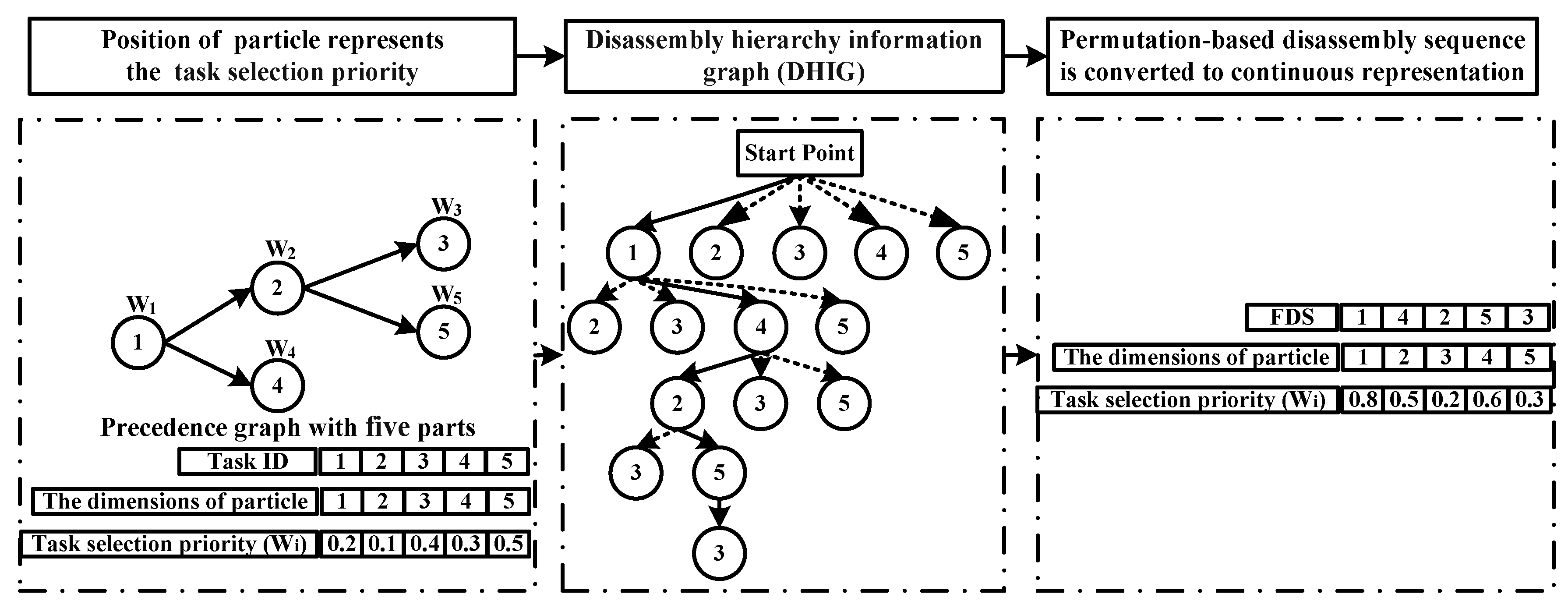
The reverse approach is performed to transform the FDS into the continuous representation for updating the proposed algorithm. We need to generate random numbers between (0, 1) as many as the number of tasks, then these numbers are sorted and placed to the column of task selection priority based on the FDS. Figure 1 shows the conversion process between the continuous representation and permutation-based disassembly sequence.
4.2. Introduction of Entropy
Combining the characteristic of FDSs, two parameters of individual-dimension-entropy and population-distribution-entropy are introduced into the proposed algorithm to balance the trade-off between exploration and exploitation. Suppose that the number of FDSs is NUM, particle dimension (D) is equal to n, Rj represents a set including the jth elements of all FDSs, bij is the number of duplicate values in the Rj and Pij = 1/bij. Relevant definitions are as follows.
Definition 1.
The individual-dimension-entropy (M) is introduced to assess the diversity of corresponding particle and the larger M is the more diversities the particle has. The particle with good diversity is denoted by pbestbin. The calculation formula is as follows:
Definition 2.
The population-distribution-entropy (H) can be introduced to reflect the diversity and evolutionary status of the population, which is defined as Equation (9):
4.3. Dimension Learning
Each dimension of particle in mostly improved PSO is updated as show in Figure 2 [22]. The updating method of corresponding to the particle dimension maybe make some particles get into the local optimum [23]. In order to improve the spatial search ability of the particle, the dimension learning strategy that different dimensions of the particle have different learning objects is adopted. The process is shown in Figure 3 where the pbestbin is added to further enhance the diversity of information between particles. pm and pc are applied to determine the number of the particle dimensions that learn from gbest, pbest and pbestbin, respectively. The improved velocity update formula is given in Equation (10):
where c1, c2 and c3 are the learning factor of the particle tracking the pbest, gbest and pbestbin respectively. r1 and r2 are uniform random number in the interval [0, 1], and w is an inertia weight.
4.4. Self-Adaptive Crossover and Mutation Operator
Based on the H, the self-adaptive crossover and mutation operator are introduced into the proposed algorithm. When H is decreased, it indicates that the individuals in the population tend to be consistent, crossover and mutation factor automatically increase in order to improve the probability of producing feasible solutions and avoid prematurity. By contrast, crossover and mutation factor automatically decrease to protect the survival of the excellent individuals. The pu and pv represent the adaptive crossover factor and mutation factor, respectively. The relationships of the crossover and mutation factor with H are as below:
where, the maximum and minimum probability of crossover and mutation are as follows: pu1, pu2, pv1 and pv2. In this study, the one-point crossover [24] and shift mutation operator [25] are used to produce the new disassembly solutions while satisfying the precedence constraints. For the implement of the one-point crossover, the two FDSs are need. Here, FDS.1 and FDS.2 are randomly selected to illustrate the crossover operation. The procedure is as follows: Firstly select a cut point in the FDSs in order to divide the FDSs into two parts and do not change the positions of the tasks before the cut position. Then, remove the tasks before the cut position in the FDS.1 from the FDS.2 whereas the tasks that are front of the cut point in the FDS.2 are removed from the FDS.1. Lastly, reconstruct two new solutions by recombining the tasks before the cut position in the FDS.1 with the remaining tasks of FDS.2 and placing the remaining tasks of FDS.1 behind the cut point in the FDS.2. The shift mutation operator is defined by randomly selecting a task in the disassembly sequence and inserting it to another randomly selected position based on the precedence matrix. By comparing the domination ability between the new solutions and current solutions, the winner will be converted to continuous representation (see Section 4.1) and replace the current particle to next generation. Examples for the one-point crossover and shift mutation operator are given in Figure 4 and Figure 5.
4.5. The Regeneration of the Particles
From a single run, the improved algorithm could obtain a set of non-dominated solutions that are used to be stored by external archive. In this paper, the size of external archive is equal to the population size and controlled by the crowding distance (CD) [18]. The obtained non-dominated solutions are converted to continuous representation as it is mentioned in Section 4.1, then considered as the pbest. If the number of non-dominated solutions is less than the population size, we will randomly select the FDSs from the external archive and take them on order crossover operation [26] for production new solutions.
There are two factors that influence the selection of gbest, that is, CD and grid density (GD) [27]. More specifically, the non-dominated solution with minimal values about the two indexes will be converted to continuous representation and then selected as the gbest.
4.6. Algorithm Proceduce for DLBP
The entire optimization procedure of proposed algorithm is repeated until the maximum generation has reached.
- Step 1:
- Set , , , , , , , , , , , , , , , , .
- Step 2:
- Built the DHIG in order to calculate the individual-dimension-entropy and the population-distribution-entropy by Equations (8) and (9), respectively. Then, select and calculate the values of and .
- Step 3:
- Update the position of particles by Equation (10).
- Step 4:
- Evaluate the objective functions.
- Step 5:
- Adopt self-adaptive crossover and mutation operator to create better solutions.
- Step 6:
- Update the external archive.
- Step 7:
- Convert the non-dominated solution to the continuous representation and replace with pbest for use at the next generation.
- Step 8:
- Make sure the position of the gbest according to the values of CD and GD.
- Step 9:
- If T > Tmax, go to step 10; else, go back to step 2.
- Step 10:
- Output optimal disassembly solutions.
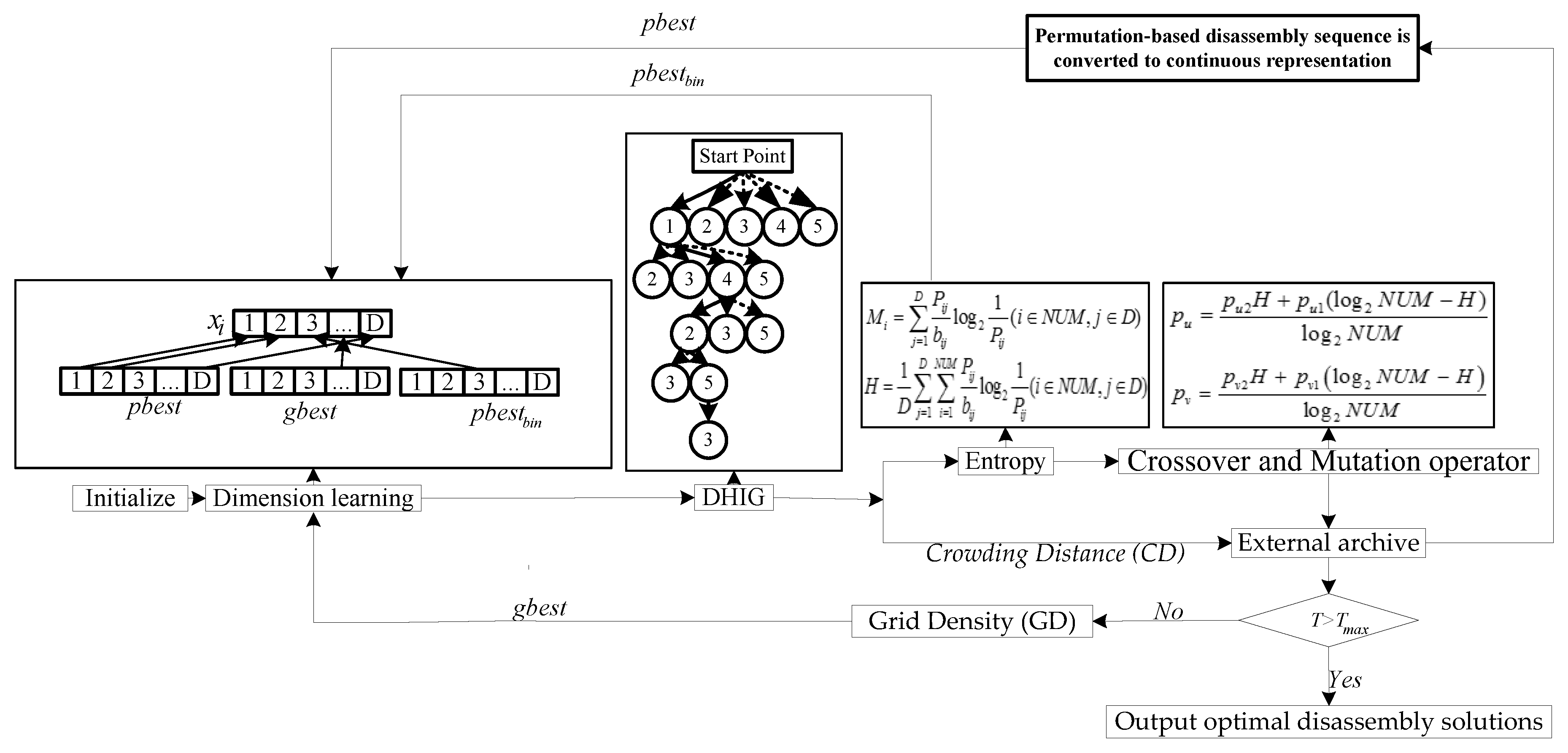
The above-mentioned procedure of the AHPSO with entropy for DLBP is just like the Figure 6.
5. Numerical Results
5.1. Test for Benchmark Functions
The DTLZ1 and DTLZ2 are used to verify the effectiveness of the multi-objective optimization algorithms. In order to show the motivation of the entropy, we make a comparison between the AHPSO without entropy and AHPSO with entropy in this section. The parameters of algorithms are listed in Table 1 and both algorithms are executed 30 times.
The Pareto optimal fronts obtained by both algorithms for solving the DTLZ1 and DTLZ2 are shown in Figure 7 and Figure 8, respectively. Generational Distance (GD), Spacing (SP) and Maximum Spread (MS) are used to measure the convergence and the coverage, respectively [28]. Table 2 lists the values of GD, SP and MS.
As can be seen from the Figure 7, both algorithms can converge to the Pareto optimal solutions, but the AHPSO with entropy is better than AHPSO without entropy in terms of the distribution of the solutions. The statistical results in Table 2 show again that AHPSO with entropy has good performance when dealing with the DTLZ1 test problem. In the Figure 8a, we can get that the Pareto optimal solutions obtained by AHPSO without entropy on DTLZ2 can’t converge to the true Pareto optimal front. The AHPSO with entropy, however, shows high convergence. The values of GD, SP and MS (see Table 2) evidence the proposed algorithm can solve the multi-objective problems well. This is due to updating mechanism of improved algorithm based on the entropy, which can measure the changing tendency of population diversity in real-time.
5.2. Applied Examples
After a set of experiments, the best performing parameter set is determined to be (population size), (the size of external archive), , , , , , , , , and these are used in benchmark instances and practical example.
Case 1: in this paper, we use a set of benchmark instances to confirm the effectiveness of improved algorithm for DLBP. The size of 19 benchmark instances increases gradually from 8 to 80 in steps of 4 and each workstation has got 26 s at most to fulfill its task. Removal time of each part is to be gained by the Equation (13). In addition, McGovern and Gupta set up that only the last part possessing removal time of 11 is hazardous and only the last part holding removal time of 7 is demanded [6]. Known optimal results are , , , and the immediately preceding matrix of each benchmark instance is an empty set [6].
This paper optimizes multi-objective simultaneously rather than based on the precedence relation between objectives. In order to compare with the DLBP ACO [6], the improved algorithm is run three times to obtain the average results and the results are evaluated in two aspects as follows:
- (1)
- Based on prioritization of multi-objective.
- (2)
- Optimize the objectives simultaneously.
The minimum number of workstations on the first four benchmark instances obtained by the proposed algorithm agrees well with the theoretical values. In the wake of increase in the number of tasks, we get the optimal solutions with workstations. The comparisons of the average results based on aspect (1) and aspect (2) are given in Figure 9, where the two curves, Data.1 and Data.2, are the average measure of the solutions based on aspect (1) and aspect (2), respectively.
From Figure 9a we can see that two curves overlap well, almost on the same line, and the computational results relating to the number of workstation are better than ACO algorithm, which got the solutions with workstations. Compared to Data.1 on the range of instance from 1th to 14th, the value of Data.2 is little higher but the performance of proposed algorithm is improved when it is used to solve instances with large size (after 14th instance, the values of Data.2 is declining).
Figure 9b shows the relation between the average balance measure and the number of task. On the whole process of 19 instances, it can be seen from Data.1 that the balance measure increases from 0 to 145.43 and then decreases until it reaches to 38.26. At the same time, the Data.2 shows a downward trend, from 180 to 39.14. After 5th instance, the values of Data.2 are less than or equal to Data.1. The average balance measures of Data.2 and ACO have similarly changing tendency, but the balance measure on the first benchmark instance obtained by McGovern and Gupta was up to 300, the minimum value was about 48. According to the analysis above, we can draw a conclusion that the proposed algorithm can acquire the satisfying results which no matter what in the aspect of basing on prioritization of multi-objective and optimizing the objectives simultaneously.
In Figure 9c, the maximal hazard measure of Data.2 is about 18 and the hazard measure is improved that overall values of Data.2 are lower in comparison with Data.1. Especially after 16th instance, the variation tendency of Data.2 decreases rapidly. We can get that the superiority of improved algorithm is much more obvious for large-size DLBP. In the ACO algorithm, the hazard measure is sub-optimally placed so it will not change if the balance measure is affected. Beyond that, it is a disappointing that hazard measure of ACO is up to around 28.
From Figure 9d, we can learn that the values of demand measure of Data.2 on the first two instances are higher than that of Data.1 but the Data.2 has a significantly lower than Data.1 with the increasing number of task. As for the ACO algorithm, the demand measure is inferior to the Data.1.
Figure 9a,b could not reflect the obvious superiority of the improved algorithm. However, hazard measure and demand measure have remarkable improvement, especially in large-size instance (as seen from Figure 9c,d). In addition, the results of the experiment show that proposed algorithm has good stability on the DLBP.
Case 2: A cellular telephone instance with 25-part (see Figure 10) defined by Gupta and McGovern [29] is used to verify the performance of the proposed algorithm. The CT is set 18 s and other knowledge databases are as follows:
- The removal times are set to
- The hazard values are quantified to
- Demands are set to
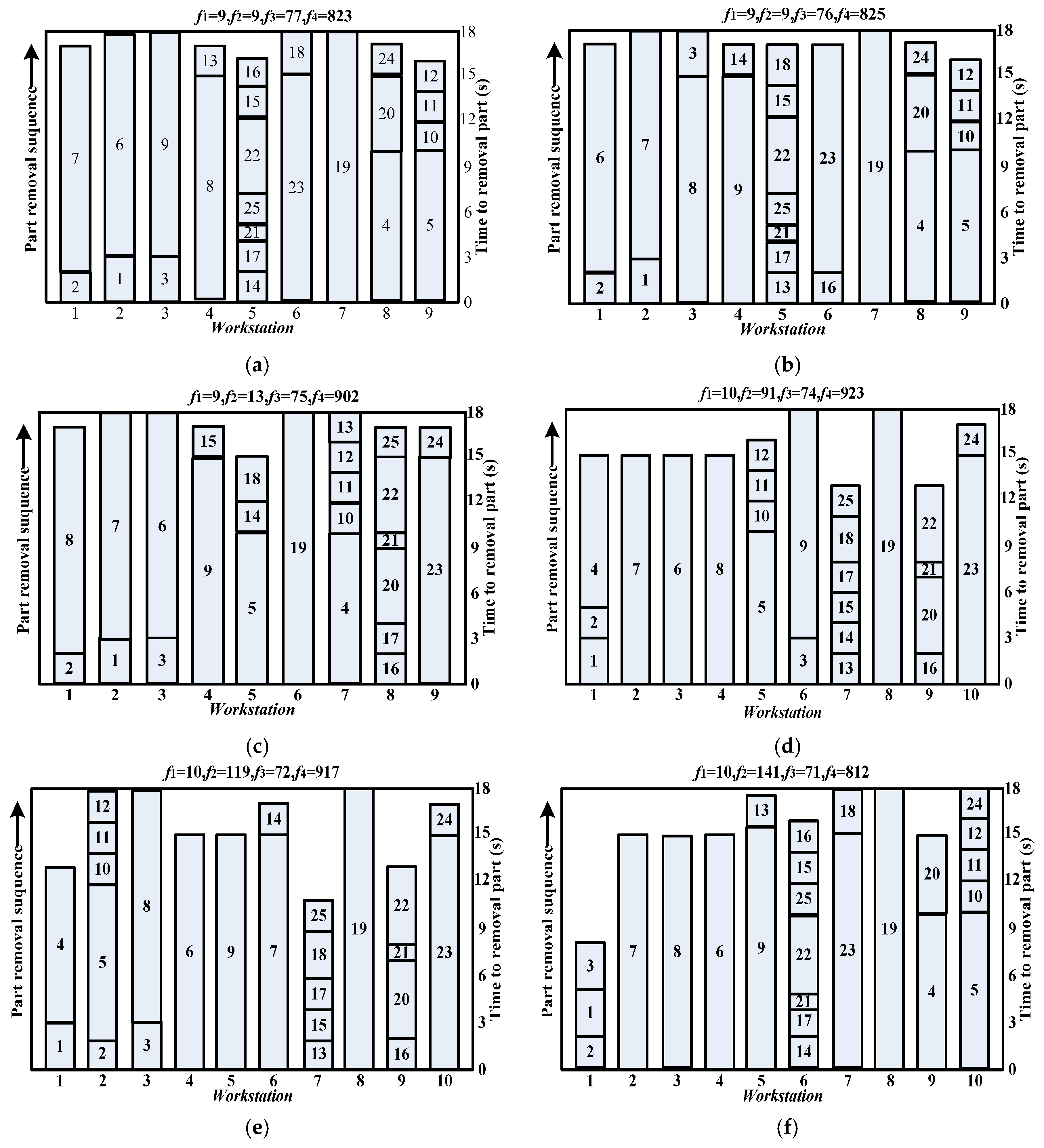
The proposed algorithm is compared with six algorithms which are GA [2], PSO [9], SA [8], VNS [10], ABC [11] and MOACO [7]. Table 3 lists the typical results of above algorithms. Six Pareto optimal solutions obtained by proposed algorithm are given in Figure 11.
According to Pareto dominance relationship, the solution by VNS dominates the results obtained by GA, PSO, SA, ABC and MOACO. From the Figure 11, the Pareto optimal solutions generated by improved algorithm can cover or surpass the current known best solutions and find more feasible solutions that the disassembly line designer can make their own decision.
From Table 3 it is clear that the minimum number of workstations in above methods is 9, the balance measure is also 9, the minimal value for the hazard measure is 76 and the minimal value for the demand measure is 825. From the (a–f) in the Figure 11, the minimal value of workstations and balance measure are 9 respectively, the minimal value of the hazard measure is 72 and the minimal value of the demand measure is 812. The average values of all non-dominated solutions found by improved algorithm are higher than above values except for the , this illustrates the conflict relationships among the objectives. Based on the above analysis, the improved algorithm has good comprehensive performance with respect to actual engineering application condition of DLBP and solution quality.
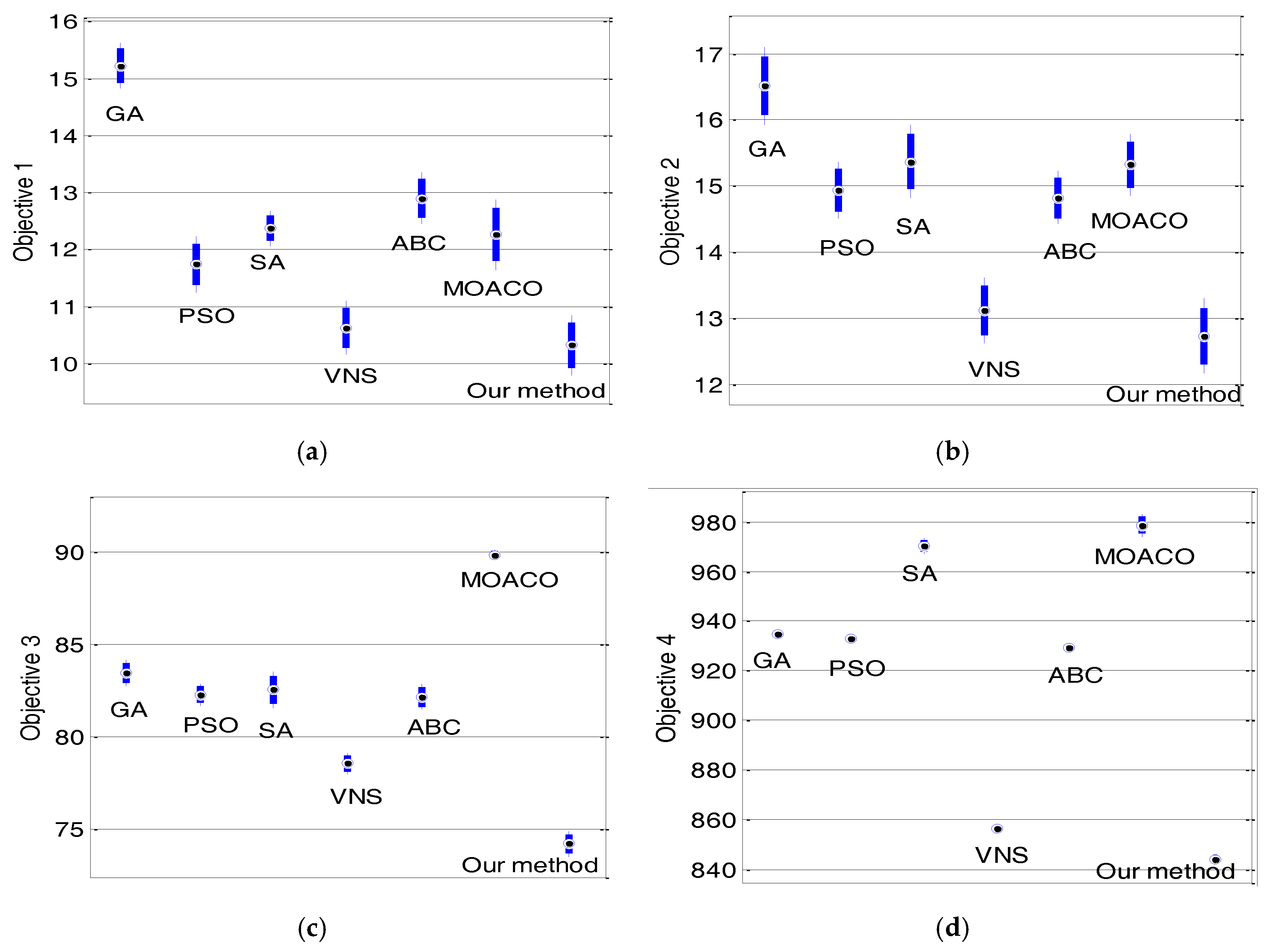
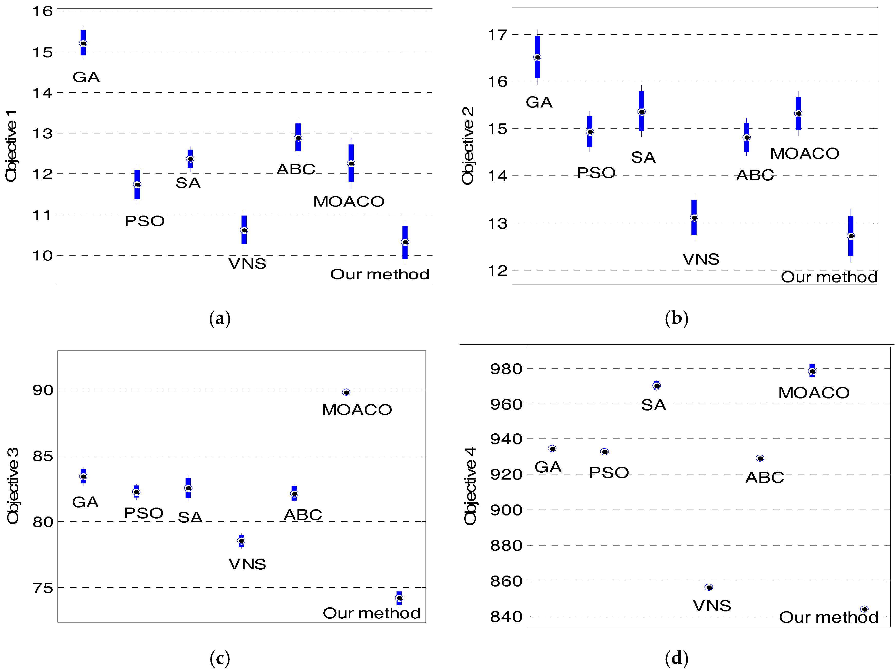
For comparison purposes, seven algorithms are executed 30 times for 25-part DLBP example under the same system configurations. The values of average, standard deviation and confidence interval within 90% for each objective are given in Table 4. The detailed results are demonstrated in Figure 12.
Although the seven algorithms can get the optimal solutions, the entropy-based AHPSO and VNS are able to reach better results than others algorithms from the overall comprehensive analysis of Figure 12. And in terms of all objectives, the performance of the entropy-based AHPSO is better than the VNS, especially about the objective 3 and objective 4 (see Figure 12c,d). As can be seen in Figure 12a,b, the performance of GA is worst when compare with other algorithms, and the performances of PSO, SA, ABS and MOACO are not significantly different. However, in terms of objective 4 (see Figure 12d), the values of confidence interval within 90% have obvious distinction. With the above analysis, we can get the entropy-based AHPSO has high stability and accuracy feature.
6. Conclusions
This paper expands the application fields of entropy and an efficient improved algorithm that entropy-based AHPSO is presented for solving DLBP. According to the characteristic of the disassembly sequence, the entropy is introduced into the proposed algorithm to measure the changing tendency of population diversity, particle with good diversity based on the entropy is selected to be added the velocity equation. In addition, the crossover and mutation factor change with the value of entropy. The computational results of the proposed algorithm for a set of benchmark instances and a practical disassembly example are compared with the typical algorithms, which show that the improved algorithm is well suited to the multi-criteria decision making problem and complicated combinatorial optimization problem. As future research directions, the AHPSO with entropy may be improved in terms of effectively constructing the initial solutions and dividing the particle dimensions into several groups by analyzing the relations among disassembly tasks.
Acknowledgments
This project is supported by the National Natural Science Fund of China (Grant No. 61403249) and Shanghai University of Engineering Science (Grand No. E309031601178).
Author Contributions
Shanli Xiao and Yujia Wang conceived and designed the entropy-based AHPSO algorithm; Shanli Xiao and Shankun Nie performed the experiments; Hui Yu and Shankun Nie analyzed the data; Shanli Xiao and Yujia Wang wrote the paper; Finally, Yujia Wang guided to modify and Shanli Xiao revised the paper. All authors have read and approved the final manuscript.
Conflicts of Interest
The authors declare no conflict of interest.
References
- Güngör, A.; Gupta, S.M. Disassembly line in product recovery. Int. J. Prod. Res. 2002, 40, 2569–2589. [Google Scholar] [CrossRef]
- McGovern, S.M.; Gupta, S.M. A balancing method and genetic algorithm for disassembly line balancing. Eur. J. Oper. Res. 2007, 179, 692–708. [Google Scholar] [CrossRef]
- Özceylan, E.; Paksoy, T. Fuzzy mathematical programming approaches for reverse supply chain optimization with disassembly line balancing problem. J. Intell. Fuzzy Syst. 2014, 26, 1969–1985. [Google Scholar]
- Mete, S.; Çil, Z.A.; Özceylan, E.; Ağpak, K. Resource constrained disassembly line balancing problem. IFAC-PapersOnLine 2016, 49, 921–925. [Google Scholar] [CrossRef]
- Altekin, F.T.; Kandiller, L.; Ozdemirel, N.E. Profit-oriented disassembly-line balancing. Int. J. Prod. Res. 2008, 46, 2675–2693. [Google Scholar] [CrossRef] [Green Version]
- McGovern, S.M.; Gupta, S.M. Ant colony optimization for disassembly sequencing with multiple objectives. Int. J. Adv. Manuf. Technol. 2006, 30, 481–496. [Google Scholar] [CrossRef]
- Ding, L.P.; Feng, Y.X.; Tan, J.R.; Gao, Y.C. A new multi-objective ant colony algorithm for solving the disassembly line balancing problem. Int. J. Adv. Manuf. Technol. 2010, 48, 761–771. [Google Scholar] [CrossRef]
- Kalayci, C.B.; Gupta, S.M.; Nakashima, K. A Simulated Annealing Algorithm for Balancing a Disassembly Line. In Design for Innovative Value towards a Sustainable Society; Springer: Berlin, Germany, 2012. [Google Scholar]
- Kalayci, C.B.; Gupta, S.M. A particle swarm optimization algorithm for solving disassembly line balancing problem. In Proceedings for the Northeast Region Decision Sciences Institute; Springer: Berlin, Germany, 2012. [Google Scholar]
- Kalayci, C.B.; Polat, O.; Gupta, S.M. A variable neighborhood search algorithm for disassembly lines. J. Manuf. Technol. Manag. 2014, 26, 182–194. [Google Scholar] [CrossRef]
- Kalayci, C.B.; Gupta, S.M.; Nakashima, K. Bees colony intelligence in al solving disassembly line balancing problem. In Proceedings of the 2011 Asian Conference of Management Science and Applications, Sanya, China, 21–23 December 2011; pp. 21–22. [Google Scholar]
- Aydemir-Karadag, A.; Turkbey, O. Multi-objective optimization of stochastic disassembly line balancing with station paralleling. Comput. Ind. Eng. 2013, 65, 413–425. [Google Scholar] [CrossRef]
- Paksoy, T.; Güngör, A.; Özceylan, E.; Hancilar, A. Mixed model disassembly line balancing problem with fuzzy goals. Int. J. Prod. Res. 2013, 51, 6082–6096. [Google Scholar] [CrossRef]
- Kalayci, C.B.; Gupta, S.M. Ant colony optimization for sequence-dependent disassembly line balancing problem. J. Manuf. Technol. Manag. 2013, 24, 413–427. [Google Scholar] [CrossRef]
- Kalayci, C.B.; Gupta, S.M. A particle swarm optimization algorithm with neighborhood-based mutation for sequence-dependent disassembly line balancing problem. Int. J. Adv. Manuf. Technol. 2013, 69, 197–209. [Google Scholar] [CrossRef]
- Kalayci, C.B.; Gupta, S.M. Artificial bee colony algorithm for solving sequence-dependent disassembly line balancing problem. Expert Syst. Appl. 2013, 40, 7231–7241. [Google Scholar] [CrossRef]
- Kalayci, C.B.; Polat, O.; Gupta, S.M. A hybrid genetic algorithm for sequence-dependent disassembly line balancing problem. Ann. Opera. Res. 2016, 242, 321–354. [Google Scholar] [CrossRef]
- Turky, A.M.; Abdullah, S. A multi-population harmony search algorithm with external archive for dynamic optimization problems. Inf. Sci. 2014, 272, 84–95. [Google Scholar] [CrossRef]
- Hu, W.; Liang, H.; Peng, C.; Du, B.; Hu, Q. A hybrid chaos-particle swarm optimization algorithm for the vehicle routing problem with time window. Entropy 2013, 15, 1247–1270. [Google Scholar] [CrossRef]
- Nasir, M.; Das, S.; Maity, D.; Sengupta, S.; Halder, U.; Suganthan, P.N. A dynamic neighborhood learning based particle swarm optimizer for global numerical optimization. Inf. Sci. 2012, 209, 16–36. [Google Scholar] [CrossRef]
- Dou, J.; Su, C.; Li, J. A discrete particle swarm optimization algorithm for assembly line balancing problem of type 1. IEEE Comput. Soc. 2011, 1, 44–47. [Google Scholar]
- Kennedy, J.; Eberhart, R. Particle swarm optimization. In Proceedings of the 1995 IEEE International Conference on Neural Networks, Perth, Western Australia, 27 November–1 December 1995; pp. 1942–1948. [Google Scholar]
- Van, D.B.F.; Engelbrecht, A.P. A cooperative approach to particle swarm optimization. IEEE Trans. Evol. Comput. 2004, 8, 225–238. [Google Scholar]
- De Paula, L.; Soares, A.S.; de Lima, T.W.; Coelho, C.J. Feature Selection using Genetic Algorithm: An analysis of the bias-property for one-point crossover. In Proceedings of the 2016 on Genetic and Evolutionary Computation Conference Companion, New York, NY, USA, 20–24 July 2016; pp. 1461–1462. [Google Scholar]
- Samuel, R.K.; Venkumar, P. Some novel methods for flow shop scheduling. Int. J. Eng. Sci. Technol. 2011, 3, 8395–8403. [Google Scholar]
- Cicirello, V.A. Non-wrapping order crossover: An order preserving crossover operator that respects absolute position. In Proceedings of the Genetic and Evolutionary Computation Conference, GECCO 2006, Seattle, WA, USA, 8–12 July 2006; pp. 1125–1132. [Google Scholar]
- Raquel, C.R.; Naval, P.C. An effective use of crowding distance in multi-objective particle swarm optimization. In Proceedings of the 7th Annual Conference on Genetic and Evolutionary Computation, Washington, DC, USA, 25–29 July 2005; pp. 257–264. [Google Scholar]
- Deb, K.; Pratap, A. A fast and elitist multi-objective genetic algorithm: NSGA-II. IEEE Trans. Evol. Comput. 2004, 8, 256–279. [Google Scholar]
- McGovern, S.M.; Gupta, S.M. Uninformed and probabilistic distributed agent combinatorial searches for the unary NP-complete disassembly line balancing problem. In Proceedings of the SPIE-The International Society for Optical Engineering, Bellingham, WA, USA, 4 November 2005; Volume 5997. [Google Scholar]
Figure 1.
The conversion process between the continuous representation and permutation-based disassembly sequence.
Figure 1.
The conversion process between the continuous representation and permutation-based disassembly sequence.

Figure 2.
Learning method of standard PSO (a) Particle learns from pbest; (b) Particle learns from gbest.
Figure 2.
Learning method of standard PSO (a) Particle learns from pbest; (b) Particle learns from gbest.
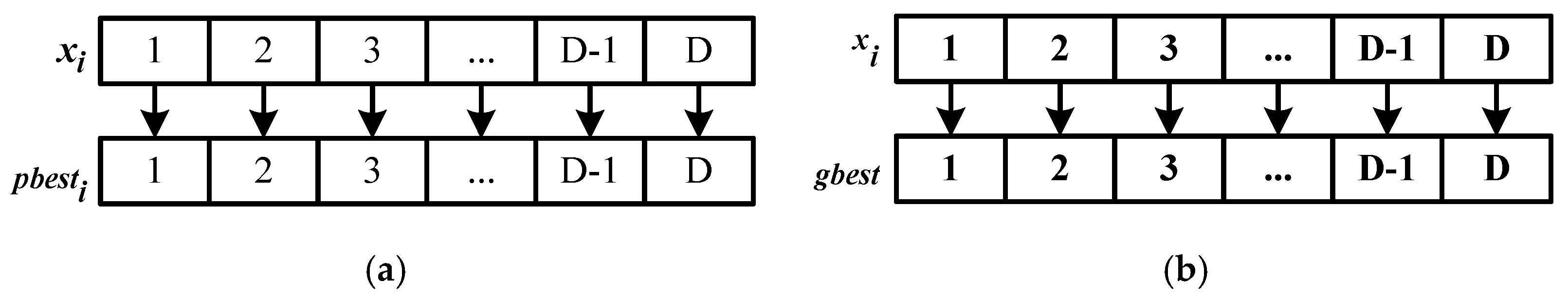
Figure 3.
The process of different learning objects for different dimensions of the particle.
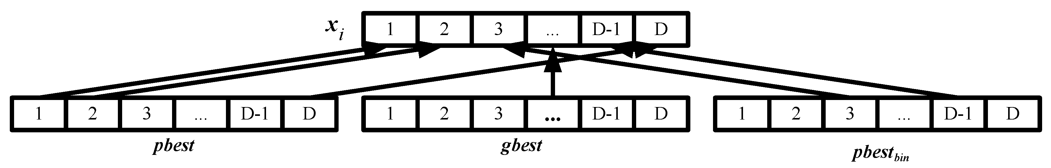
Figure 4.
Applying the one-point crossover to assign five-part example.

Figure 5.
Applying the shift mutation operator to assign five-part example.
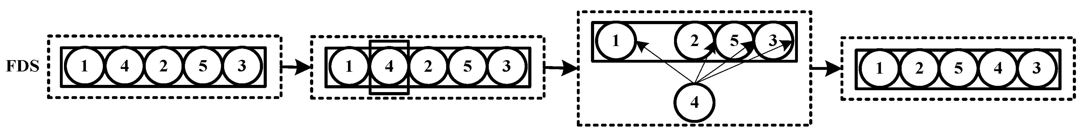
Figure 6.
Procedure of the proposed algorithm for DLBP.

Figure 7.
Obtained Pareto optimal fronts on DTLZ1 (a) AHPSO without entropy; (b) AHPSO with entropy.
Figure 7.
Obtained Pareto optimal fronts on DTLZ1 (a) AHPSO without entropy; (b) AHPSO with entropy.
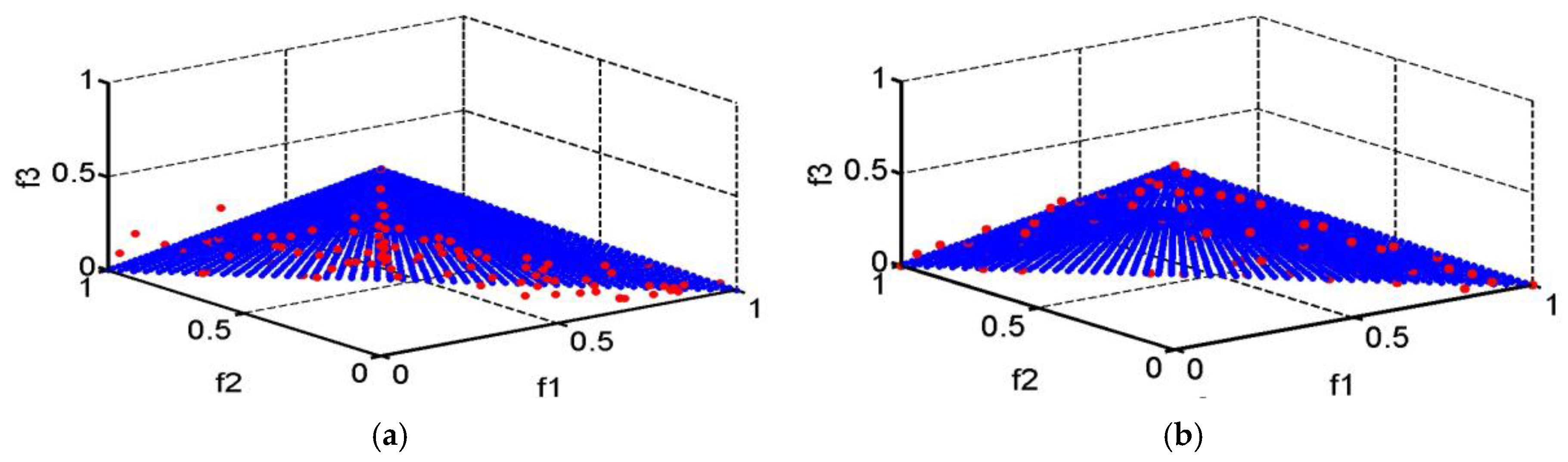
Figure 8.
Obtained Pareto optimal fronts on DTLZ2 (a) AHPSO without entropy; (b) AHPSO with entropy.
Figure 8.
Obtained Pareto optimal fronts on DTLZ2 (a) AHPSO without entropy; (b) AHPSO with entropy.
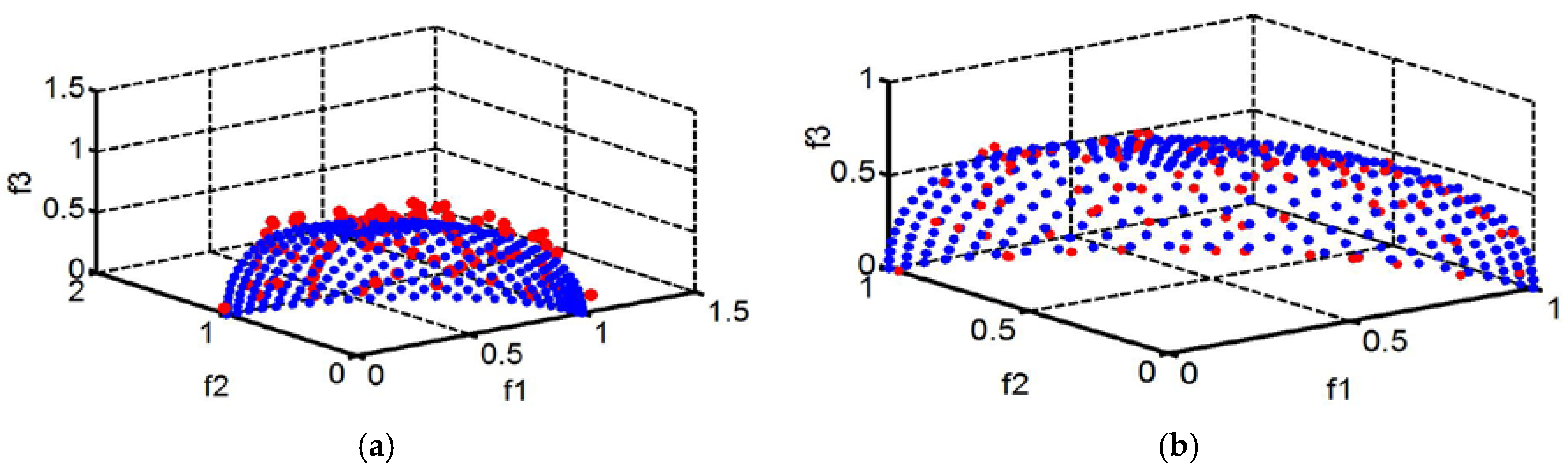
Figure 9.
The comparisons of the average results on different measures (a) Number of workstations; (b) Balance measure; (c) Hazard measure; (d) Demand measure.
Figure 9.
The comparisons of the average results on different measures (a) Number of workstations; (b) Balance measure; (c) Hazard measure; (d) Demand measure.
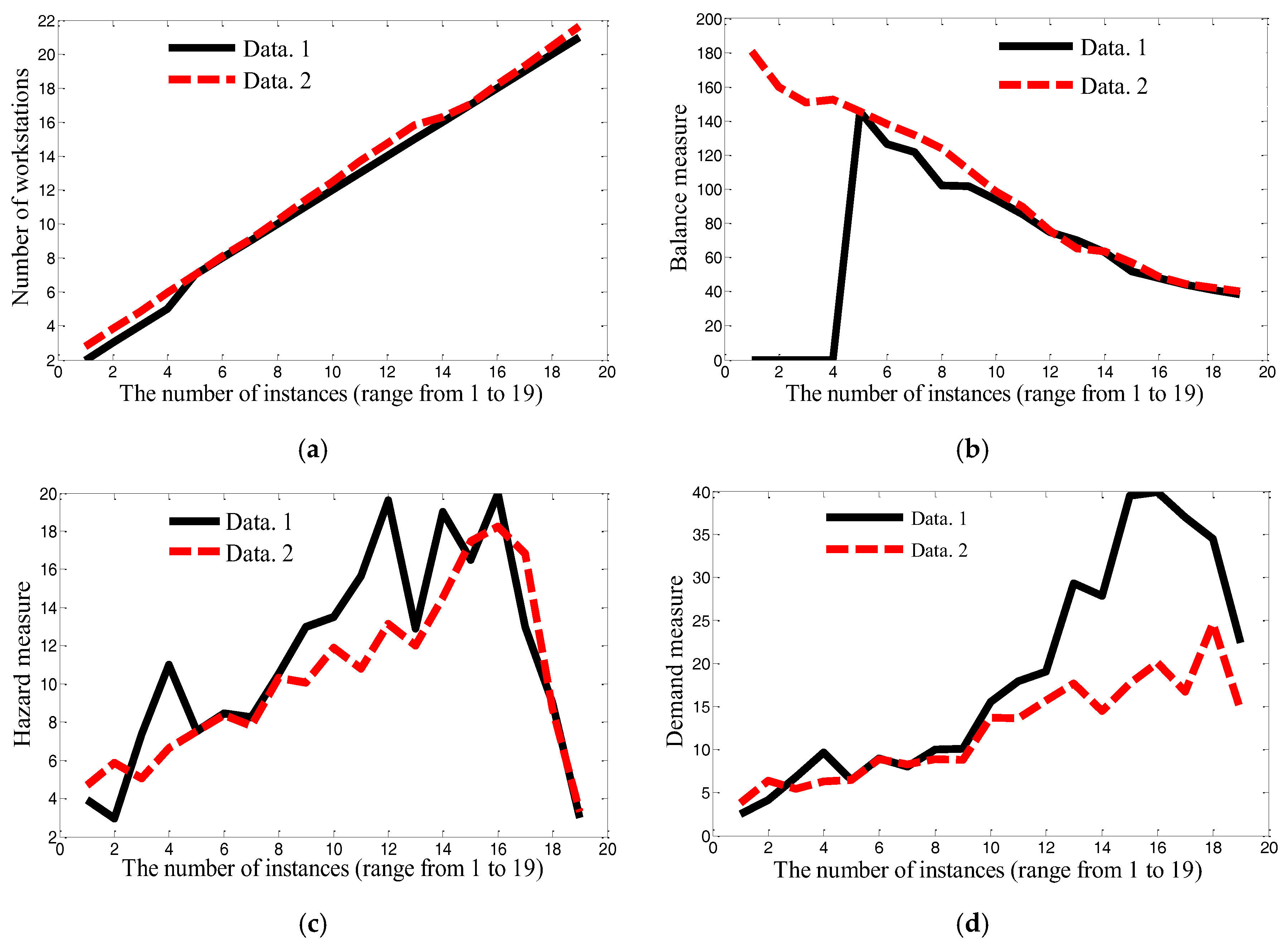
Figure 10.
Precedence relationships for cellular telephone.

Figure 11.
Pareto optimal solutions of 25-part DLBP example (a) solution 1; (b) solution 2; (c) solution 3; (d) solution 4; (e) solution 5; (f) solution 6.
Figure 11.
Pareto optimal solutions of 25-part DLBP example (a) solution 1; (b) solution 2; (c) solution 3; (d) solution 4; (e) solution 5; (f) solution 6.

Figure 12.
Performance comparison of the proposed algorithm within 90% confidence interval (a) Objective 1; (b) Objective 2; (c) Objective 3; (d) Objective 4.
Figure 12.
Performance comparison of the proposed algorithm within 90% confidence interval (a) Objective 1; (b) Objective 2; (c) Objective 3; (d) Objective 4.

Table 1.
Parameters setting.
| Type | AHPSO without Entropy | AHPSO with Entropy |
|---|---|---|
| The particle with good diversity | Randomly selected one from the other particles’ | |
| Crossover rate and mutation rate | According to Equations (11) and (12) | Empirical value: , |
| Inertia weight | ||
| Learning factor | ||
| The size of external archive | 100 | 100 |
| 100 | 100 | |
| / | , | , |
| 30 | 30 | |
| 300 | 300 |
Table 2.
The values of GD, SP and MS on the DTLZ1 and DTLZ2.
| Performance Metric | AHPSO without Entropy | AHPSO with Entropy | |
|---|---|---|---|
| DTLZ1 | GD | 5.1445 × 10⁻⁴ | 1.3342 × 10⁻⁴ |
| SP | 0.0055 | 0.0042 | |
| MS | 0.9878 | 1 | |
| DTLZ2 | GD | 3.701 × 10⁻⁴ | 2.403 × 10⁻⁴ |
| SP | 0.0063 | 0.0045 | |
| MS | 0.9842 | 0.9967 |
Table 3.
Comparison of the typical results for 25-part DLBP example.
| Publication | Method | f1 | f2 | f3 | f4 | |
|---|---|---|---|---|---|---|
| McGovern and Gupta, 2007 [2] | GA | 9 | 9 | 82 | 868 | |
| Kalayci and Gupta, 2012 [9] | PSO | 9 | 9 | 80 | 857 | |
| Kalayci and Gupta, 2012 [8] | SA | 9 | 9 | 81 | 853 | |
| Kalayci et al., 2014 [10] | VNS | 9 | 9 | 76 | 825 | |
| Kalayciet al., 2011 [11] | ABC | 9 | 9 | 81 | 853 | |
| Ding et al., 2010 [7] | MOACO | No.1 | 9 | 9 | 87 | 927 |
| No.2 | 9 | 11 | 85 | 898 | ||
Table 4.
Performance comparison of seven algorithms for 25-part disassembly.
| Objective | Method | Average | Standard Deviation | Confidence Interval | |
|---|---|---|---|---|---|
| f1 | GA | 15.22 | 1.34 | 14.82 | 15.62 |
| PSO | 11.74 | 1.64 | 11.25 | 12.23 | |
| SA | 12.37 | 1.01 | 12.07 | 12.67 | |
| VNS | 10.63 | 1.56 | 10.16 | 11.10 | |
| ABC | 12.9 | 1.52 | 12.44 | 13.35 | |
| MOACO | 12.26 | 2.07 | 11.64 | 12.88 | |
| entropy-based AHPSO | 10.32 | 1.72 | 9.80 | 10.84 | |
| f2 | GA | 16.51 | 1.98 | 15.92 | 17.10 |
| PSO | 14.94 | 1.43 | 14.51 | 15.37 | |
| SA | 15.37 | 1.87 | 14.81 | 15.93 | |
| VNS | 13.12 | 1.64 | 12.63 | 13.61 | |
| ABC | 14.82 | 1.34 | 14.42 | 15.22 | |
| MOACO | 15.32 | 1.55 | 14.85 | 15.79 | |
| entropy-based AHPSO | 12.74 | 1.89 | 12.17 | 13.30 | |
| f3 | GA | 83.46 | 2.37 | 82.75 | 84.17 |
| PSO | 82.27 | 1.98 | 81.68 | 82.86 | |
| SA | 82.53 | 3.35 | 81.52 | 83.54 | |
| VNS | 78.55 | 1.93 | 77.97 | 79.13 | |
| ABC | 82.15 | 2.30 | 81.46 | 82.84 | |
| MOACO | 89.83 | 0.93 | 89.55 | 90.11 | |
| entropy-based AHPSO | 74.2 | 2.31 | 73.51 | 74.89 | |
| f4 | GA | 934.64 | 6.72 | 932.62 | 936.66 |
| PSO | 932.81 | 5.38 | 931.19 | 934.43 | |
| SA | 970.35 | 10.54 | 967.18 | 973.52 | |
| VNS | 856.29 | 4.87 | 854.83 | 857.75 | |
| ABC | 929.43 | 5.09 | 927.90 | 930.96 | |
| MOACO | 978.67 | 15.02 | 974.16 | 983.18 | |
| entropy-based AHPSO | 843.82 | 5.96 | 842.03 | 845.61 | |
© 2017 by the authors. Licensee MDPI, Basel, Switzerland. This article is an open access article distributed under the terms and conditions of the Creative Commons Attribution (CC BY) license (http://creativecommons.org/licenses/by/4.0/).
Share and Cite
MDPI and ACS Style
Xiao, S.; Wang, Y.; Yu, H.; Nie, S. An Entropy-Based Adaptive Hybrid Particle Swarm Optimization for Disassembly Line Balancing Problems. Entropy 2017, 19, 596. https://doi.org/10.3390/e19110596
AMA Style
Xiao S, Wang Y, Yu H, Nie S. An Entropy-Based Adaptive Hybrid Particle Swarm Optimization for Disassembly Line Balancing Problems. Entropy. 2017; 19(11):596. https://doi.org/10.3390/e19110596
Chicago/Turabian StyleXiao, Shanli, Yujia Wang, Hui Yu, and Shankun Nie. 2017. "An Entropy-Based Adaptive Hybrid Particle Swarm Optimization for Disassembly Line Balancing Problems" Entropy 19, no. 11: 596. https://doi.org/10.3390/e19110596
Note that from the first issue of 2016, this journal uses article numbers instead of page numbers. See further details here.