Maximum Correntropy Criterion Kalman Filter for α-Jerk Tracking Model with Non-Gaussian Noise

Abstract

As one of the most critical issues for target track, $\alpha$-jerk model is an effective maneuver target track model. Non-Gaussian noises always exist in the track process, which usually lead to inconsistency and divergence of the track filter. A novel Kalman filter is derived and applied on $\alpha$-jerk tracking model to handle non-Gaussian noise. The weighted least square solution is presented and the standard Kalman filter is deduced firstly. A novel Kalman filter with the weighted least square based on the maximum correntropy criterion is deduced. The robustness of the maximum correntropy criterion is also analyzed with the influence function and compared with the Huber-based filter, and, moreover, the kernel size of Gaussian kernel plays an important role in the filter algorithm. A new adaptive kernel method is proposed in this paper to adjust the parameter in real time. Finally, simulation results indicate the validity and the efficiency of the proposed filter. The comparison study shows that the proposed filter can significantly reduce the noise influence for $\alpha$-jerk model.

1. Introduction

Target track is a real-time estimation process to obtain the position, the velocity and other motion parameters for the tracked target through the measurement data. Because of the uncertainty and nonlinearity of the maneuver target motion process and the target measurement process, a lot of algorithms were researched and proposed for the maneuver target track in the past [1,2]. To sum up, the track algorithms study has been focused on two parts, i.e., maneuver target modeling and nonlinear filter design.

For the maneuver target modeling, many models were proposed to describe the target maneuvers. Singer model [3] is a classic model proposed by Singer in 1970. In 1982, Bar-shalom and Birmiwal [4] proposed a maneuver target track model with the maneuver detection. In 1984, Zhou and Kumar [5] proposed the current statistical model based on the Singer model. The jerk model proposed by Mehrotra [6] was another valid method to track the maneuver target. Among the models above, jerk model has the highest order. A higher model order can present higher mobility of target. Jerk model broadens the adaptive target maneuver form and is more suitable for high maneuver targets [5]. However, for the traditional jerk model, “jerk” $\alpha$ should be predefined and may be time-varying in the practical process. Therefore, Luo proposed $\alpha$-jerk model [7], which considered $\alpha$ as a parameter to be estimated by the expanding-dimension method in the real-time filter process.

For the nonlinear filter design, a lot of techniques were proposed according to the different optimization rules, including the function approximation, the posteriori probability density approximation and the stochastic model approximation [8,9,10,11]. Extended Kalman Filter (EKF) is a typical technique of the function approximation based on Taylor series expansion. Unscented Kalman Filter (UKF) is the most common way of the sampling-based moment approximation [12,13]. The stochastic model approximation [14] can approximate the nonlinear function in some probabilistic senses. However, it has not gained popularity mainly because the expectations involved are not easy to evaluate. No matter what nonlinear filter methods are used, they are applied on the state estimation with Gaussian white noises in most time.

However, in practical applications, especially in the maneuver target track system, non-Gaussian noises do exist and have substantial effects on the state estimation. Up to now, some practical models are proposed, such as Gaussian mixture noise model [15], glint noise model [16] and so on.

In a non-Gaussian process, the performance of many nonlinear filters can break down [17]. However, the filter robustness against non-Gaussian noises can be improved by the following approaches:

• The first approach is to develop filters for the systems with non-Gaussian noises directly. Noise distributions such as heavy-tailed distributions and t-distributions are considered in these filters [18,19]. However, it is difficult to handle more than one dimension, which limits its applicability [20].
• Approximating the posteriori probability density is another practical approach to handle the non-Gaussian noises. The unscented Kalman filter (UKF) uses the unscented transformation (UT) technique to capture the mean and the covariance of the state estimation with sigma points [21]. The ensemble Kalman filter (EnKF) is a method to approximate the state estimation with a set of samples to handle non-Gaussian noises [22]. Gaussian sum filter (GSF) is an algorithm to obtain the filtering distribution and the predictive distribution recursively approximated as Gaussian mixtures [23,24,25].
• Huber-based robust filter is a classical method to handle the non-Gaussian noises and outliers [26]. It has become the research focus these past several years and been applied in the field of the navigation and the target track [27,28,29,30].
• A new robust Kalman filter is proposed by Chang [31] in recent years. It handles the outliers based on the hypothesis testing theory, which defines a judging index as the square of the Mahalanobis distance from the observation to its prediction. It can effectively resist the heavy-tailed distribution of the observation noises and the outliers in the actual observations.
• Multi-sensor data fusion Kalman filter is a fuzzy logical method proposed by Rodger [32]. It can effectively improve the computational burden and the robustness of Kalman filter. Furthermore, it has been applied on the vehicle health maintenance system.
• Maximum correntropy criterion is the latest optimization criterion that is used for improving Kalman filter. Maximum correntropy Kalman filter (MCKF) is a newly proposed filter to process the non-Gaussian noises [33]. In addition, several improved MCKF algorithms have been proposed and applied on state estimation [34,35,36,37].

Maximum correntropy criterion Kalman filter (MCCKF) [20] is the latest approach to handle the non-Gaussian noises with Gaussian kernel. It is different from the MCKF in the form and the derivation process. The aforementioned MCCKF has been proved to have higher accuracy than other approaches in a benchmark navigation problem with the non-Gaussian noises. However, it does not have an optimal rule for the kernel size selection, which is important for the robustness of MCCKF. Furthermore, it has not been applied on the maneuver target track. Thus, we adopt the Kalman filter based on the maximum correntropy criterion for $\alpha$-jerk model with the non-Gaussian process to realize the maneuver target track.

The key contributions of this paper are as follows. Firstly, the robustness of Kalman filter algorithm based on the maximum correntropy criterion is introduced in the presence of the non-Gaussian noises. Then, the influence function of the filter algorithm, for the first time, is analyzed in this paper. Moreover, an optimal kernel size is obtained by a novel adaptive size adjusting skill. Finally, the large outliers and the Gaussian mixture noises in the maneuver target track with $\alpha$-jerk model are properly handled by MCCKF.

The organization of this paper proceeds as follows. The $\alpha$-jerk model is briefly reviewed in Section 2. In Section 3, we design the algorithm steps for MCCKF, analyze the robustness performance with the influence function and propose a novel kernel size selection method. In Section 4, simulation results are presented to compare the performances of different filter algorithms with respect to different noise conditions. Finally, conclusions are drawn in Section 5.

2. $\mathit{\alpha }$-Jerk Model

Jerk model is a classical target tracking model. “Jerk” means the acceleration rate [6]. It is described as follows:

$$\begin{array}{c}\dot{j}\left(t\right)=-\alpha j\left(t\right)+\omega \left(t\right),\end{array}$$

(1)

where $j\left(t\right)=\stackrel{⃛}{x}\left(t\right)$ is the target “jerk”, $x\left(t\right)$ is the target position, $\alpha$ is the correlation parameter permitting the modeling of different classes of targets, $\omega \left(t\right)$ is the process noises with the zero mean and the variance ${\sigma }_{\omega }^2=2\alpha {\sigma }_j^2$, and ${\sigma }_j^2$ is the variance for the target “jerk”. In the model, $\alpha$ is a fixed value. However, it is difficult to predefine and may be time-varying in the practical process.

$\alpha$-jerk model considers $\alpha$ as a parameter to be estimated and supposes that $\alpha$ is a state variable. In this way, it will be real-time estimated in the filter process. Consider the following equation:

$$\begin{array}{c}\dot{\alpha }\left(t\right)=\epsilon \left(t\right),\end{array}$$

(2)

where $\epsilon \left(t\right)$ denotes the zero mean Gaussian noises with the variance ${\sigma }_{\epsilon }^2$.

Combined with Equation (2) and Jerk model [6], the state equation for the continuous time $\alpha$-jerk when only one variable, x, in the state variable vector ${\left[\begin{array}{ccc}x& y& z\end{array}\right]}^{\mathrm{T}}$, is considered, the $\alpha$-jerk model can be written as

$$\begin{array}{c}\frac{d}{dt}\left[\begin{array}{c}x\\ \dot{x}\\ \ddot{x}\\ \stackrel{⃛}{x}\\ \alpha \end{array}\right]=\left[\begin{array}{ccccc}0& 1& 0& 0& 0\\ 0& 0& 1& 0& 0\\ 0& 0& 0& 1& 0\\ 0& 0& 0& -\alpha & 0\\ 0& 0& 0& 0& 0\end{array}\right]\left[\begin{array}{c}x\\ \dot{x}\\ \ddot{x}\\ \stackrel{⃛}{x}\\ \alpha \end{array}\right]+\left[\begin{array}{c}0\\ 0\\ 0\\ \omega \left(t\right)\\ \epsilon \left(t\right)\end{array}\right],\end{array}$$

(3)

where x,$\dot{x}$,$\ddot{x}$,$\stackrel{⃛}{x}$ represent the position, the velocity, the acceleration and the jerk of the aerial target in the x-direction, respectively. Denote

$$\begin{array}{c}\left\{\begin{array}{c}\mathit{X}={\left[\begin{array}{ccccc}x& \dot{x}& \ddot{x}& \stackrel{⃛}{x}& \alpha \end{array}\right]}^{\mathrm{T}}\hfill \\ \mathit{W}\left(t\right)={\left[\begin{array}{ccccc}0& 0& 0& \omega \left(t\right)& \epsilon \left(t\right)\end{array}\right]}^{\mathrm{T}}\hfill \end{array}\right.\end{array}$$

(4)

and

$$\begin{array}{c}\mathbf{A}=\left[\begin{array}{ccccc}0& 1& 0& 0& 0\\ 0& 0& 1& 0& 0\\ 0& 0& 0& 1& 0\\ 0& 0& 0& -\alpha & 0\\ 0& 0& 0& 0& 0\end{array}\right].\end{array}$$

(5)

The state equation can be expressed as:

$$\begin{array}{c}\dot{\mathit{X}}=\mathit{AX}+\mathit{W}\left(t\right).\end{array}$$

(6)

Equation (6) is discretized as:

$$\begin{array}{c}{\mathit{X}}_k={\mathbf{\Phi }}_{k|k-1}{\mathit{X}}_{k-1}+{\mathit{W}}_k,\end{array}$$

(7)

where

$$\begin{array}{c}{\mathbf{\Phi }}_{k|k-1}=exp\left(\mathit{A}T\right),\end{array}$$

(8)

where T is the time interval and ${\mathbf{\Phi }}_{k|k-1}$ is the state transition matrix; ${\mathit{W}}_k$ is the process noises at time k.

From Equation (8), the discrete state transition matrix can be written as:

$$\begin{array}{c}{\mathbf{\Phi }}_{k|k-1}=\left[\begin{array}{ccccc}1& T& T^2/2& p_1& 0\\ 0& 1& T& q_1& 0\\ 0& 0& 1& r_1& 0\\ 0& 0& 0& s_1& 0\\ 0& 0& 0& 0& 1\end{array}\right],\end{array}$$

(9)

where

$$\begin{array}{c}\begin{array}{c}{p}_1=\left(2-2\alpha T+{\alpha }^2{T}^2-2e^{-\alpha T}\right)/\left(2{\alpha }^3\right)\hfill \\ q_1=\left(e^{-\alpha T}-1+\alpha T\right)/{\alpha }^2\hfill \\ r_1=\left(1-e^{-\alpha T}\right)/\alpha \hfill \\ s_1=e^{-\alpha T}\hfill \end{array}.\end{array}$$

(10)

The variance of the process noises ${\mathit{W}}_k$ is

$$\begin{array}{c}\mathit{Q}\left(k\right)=\left[\begin{array}{ccccc}{q}_{11}{\sigma }_{\omega }^2& q_{12}{\sigma }_{\omega }^2& q_{13}{\sigma }_{\omega }^2& q_{14}{\sigma }_{\omega }^2& 0\\ q_{21}{\sigma }_{\omega }^2& q_{22}{\sigma }_{\omega }^2& q_{23}{\sigma }_{\omega }^2& q_{24}{\sigma }_{\omega }^2& 0\\ q_{31}{\sigma }_{\omega }^2& q_{32}{\sigma }_{\omega }^2& q_{33}{\sigma }_{\omega }^2& q_{34}{\sigma }_{\omega }^2& 0\\ q_{41}{\sigma }_{\omega }^2& q_{42}{\sigma }_{\omega }^2& q_{43}{\sigma }_{\omega }^2& q_{44}{\sigma }_{\omega }^2& 0\\ 0& 0& 0& 0& T{\sigma }_{\epsilon }^2\end{array}\right],\end{array}$$

(11)

where

$$\begin{array}{c}\begin{array}{c}{q}_{11}=\left(1/2{\alpha }^7\right)\left({\alpha }^5{T}^5/10-{\alpha }^4{T}^4/2+4{\alpha }^3{T}^3/3\right.\hfill \\ \left.+2\alpha T-2{\alpha }^2{T}^2-3+4e^{-\alpha T}+2{\alpha }^2{T}^2{e}^{-\alpha T}-e^{-2\alpha T}\right)\hfill \\ q_{12}=q_{21}=\left(1/2{\alpha }^6\right)\left(1-2\alpha T+2{\alpha }^2{T}^2-{\alpha }^3{T}^3+{\alpha }^4{T}^4/4\right.\hfill \\ \left.+e^{-2\alpha T}+2\alpha T{e}^{-\alpha T}-2e^{-\alpha T}-{\alpha }^2{T}^2{e}^{-\alpha T}\right)\hfill \\ q_{13}=q_{31}=\left(1/2{\alpha }^5\right)\left({\alpha }^3{T}^3/3+2\alpha T-{\alpha }^2{T}^2-3\right.\hfill \\ \left.+4e^{-\alpha T}+{\alpha }^2{T}^2{e}^{-\alpha T}-e^{-2\alpha T}\right)\hfill \\ q_{14}=q_{41}=\left(1/2{\alpha }^4\right)\left(1-2e^{-\alpha T}-{\alpha }^2{T}^2{e}^{-\alpha T}+e^{-2\alpha T}\right)\hfill \\ q_{22}=\left(1/2{\alpha }^5\right)\left(1-e^{-2\alpha T}+2{\alpha }^3{T}^3/3+2\alpha T-2{\alpha }^2{T}^2-4\alpha T{e}^{-\alpha T}\right)\hfill \\ q_{23}=q_{32}=\left(1/2{\alpha }^4\right)\left(1-2\alpha T+{\alpha }^2{T}^2+2\alpha T{e}^{-\alpha T}+e^{-2\alpha T}-2e^{-\alpha T}\right)\hfill \\ q_{24}=q_{42}=\left(1/2{\alpha }^3\right)\left(1-2\alpha T{e}^{-2\alpha T}-e^{-2\alpha T}\right)\hfill \\ q_{33}=\left(1/2{\alpha }^3\right)\left(4e^{-\alpha T}+2\alpha T-e^{-2\alpha T}-3\right)\hfill \\ q_{34}=q_{43}=\left(1/2{\alpha }^2\right)\left(1-2e^{-\alpha T}+e^{-2\alpha T}\right)\hfill \\ q_{44}=\left(1/2\alpha \right)\left(1-e^{-2\alpha T}\right).\hfill \end{array}\end{array}$$

(12)

The measurement equation can be expressed as:

$$\begin{array}{c}{\mathit{Z}}_k={\mathit{H}}_k{\mathit{X}}_k+{\mathit{V}}_k,\end{array}$$

(13)

where ${\mathit{H}}_k$ is the measurement matrix at time k; ${\mathit{V}}_k$ is the measurement noises and independent of the process noises ${\mathit{W}}_k$.

In most situations, ${\mathit{V}}_k$ is the Gaussian white noises. However, in practice, due to the target glint, the scattering of the radar tracking equipment and the faults of the operators [16,38] and so on, the measurement noises may be non-Gaussian or some outliers exist in the measurement data. It can behave as:

$$\begin{array}{c}{\mathit{V}}_k={\mathit{V}}_k^{\left(1\right)}+{\mathit{V}}_k^{\left(2\right)}\end{array}$$

(14)

or

$$\begin{array}{c}{\mathit{V}}_k={\mathit{V}}_k^{\left(1\right)}+\Delta {\mathit{V}}_k,\end{array}$$

(15)

where ${\mathit{V}}_k^{\left(1\right)}$ denotes the Gaussian white noises, ${\mathit{V}}_k^{\left(2\right)}$ obeys another Gaussian distribution different from ${\mathit{V}}_k^{\left(1\right)}$, and $\Delta {\mathit{V}}_k$ denotes the outliers.

In this paper, a new filter algorithm will be proposed to deal with the non-Gaussian noises like Equations (14) and (15).

3. Design for Maximum Correntropy Criterion Kalman Filter with Non-Gaussian Noise

3.1. Standard Kalman Filter

From Section 2, $\alpha$-jerk model for the maneuver target track can be expressed as:

$$\begin{array}{c}\left\{\begin{array}{c}{\mathit{X}}_k={\mathbf{\Phi }}_{k|k-1}{\mathit{X}}_{k-1}+{\mathit{W}}_k,\hfill \\ {\mathit{Z}}_k={\mathit{H}}_k{\mathit{X}}_k+{\mathit{V}}_k.\hfill \end{array}\right.\end{array}$$

(16)

Assume ${\mathit{W}}_k$ and ${\mathit{V}}_k$ are independent Gaussian white noises, satisfying

$$\begin{array}{c}\mathrm{E}({\mathit{W}}_k{\mathit{W}}_j^{\mathrm{T}})=\left\{\begin{array}{cc}{\mathit{Q}}_k,& k=j,\\ 0,& k\ne j,\end{array}\right.,\mathrm{E}({\mathit{V}}_k{\mathit{V}}_j^{\mathrm{T}})=\left\{\begin{array}{cc}{\mathit{R}}_k,& k=j,\\ 0,& k\ne j,\end{array}\right.\end{array}$$

(17)

where ${\mathit{Q}}_k$ and ${\mathit{R}}_k$ are known positive definite matrix.

In the KF, the predicted state ${\widehat{\mathit{X}}}_{k|k-1}$ satisfies

$$\begin{array}{c}\mathrm{E}\left[\left({\mathit{X}}_k-{\widehat{\mathit{X}}}_{k|k-1}\right){\left({\mathit{X}}_k-{\widehat{\mathit{X}}}_{k|k-1}\right)}^{\mathrm{T}}\right]={\mathit{P}}_{k|k-1},\end{array}$$

(18)

where ${\mathit{P}}_{k|k-1}$ is the predicted covariance. One very reasonable estimate ${\mathit{X}}_k$, taking into account the measurement ${\mathit{Z}}_k$, is the weighted least squares estimate, which we call ${\widehat{\mathit{X}}}_k$. For this estimate, we choose ${\widehat{\mathit{X}}}_k$ as the value of ${\mathit{X}}_k$ that minimizes the quadratic form

$$\begin{array}{c}\begin{array}{c}J=\frac{1}{2}\left[{\left({\mathit{X}}_k-{\widehat{\mathit{X}}}_{k|k-1}\right)}^{\mathrm{T}}{\mathit{P}}_{k|k-1}^{-1}\left({\mathit{X}}_k-{\widehat{\mathit{X}}}_{k|k-1}\right)\right.\hfill \\ \left.+{\left({\mathit{Z}}_k-{\mathit{H}}_k{\mathit{X}}_k\right)}^{\mathrm{T}}{\mathit{R}}_k^{-1}\left({\mathit{Z}}_k-{\mathit{H}}_k{\mathit{X}}_k\right)\right].\hfill \end{array}\end{array}$$

(19)

Note that the weighting matrices, ${\mathit{P}}_{k|k-1}^{-1}$ and ${\mathit{R}}_k^{-1}$, are the inverse matrices of the prior expectations of $\left({\mathit{X}}_k-{\widehat{\mathit{X}}}_{k|k-1}\right){\left({\mathit{X}}_k-{\widehat{\mathit{X}}}_{k|k-1}\right)}^{\mathrm{T}}$ and $\left({\mathit{Z}}_k-{\mathit{H}}_k{\mathit{X}}_k\right){\left({\mathit{Z}}_k-{\mathit{H}}_k{\mathit{X}}_k\right)}^{\mathrm{T}}$, respectively, and the predicted state is obtained as follows:

$$\begin{array}{c}{\widehat{\mathit{X}}}_{k|k-1}={\mathbf{\Phi }}_{k|k-1}{\mathit{X}}_{k-1}.\end{array}$$

(20)

The value ${\widehat{\mathit{X}}}_k=arg{\displaystyle \underset{{\mathit{X}}_k}{min}}J\left({\mathit{X}}_k\right)$ will be the best estimate. The detailed proof is given in [39] to show that Kalman filter can be deduced by Equation (19).

Therefore, Kalman filter can be deduced by solving

$$\begin{array}{c}\frac{\partial J}{\partial {\widehat{\mathit{X}}}_k}=0.\end{array}$$

(21)

Therefore, Kalman filter equations are expressed as:

$$\begin{array}{c}\begin{array}{c}{\widehat{\mathit{X}}}_{k|k-1}={\mathbf{\Phi }}_{k|k-1}{\widehat{\mathit{X}}}_{k-1}\hfill \\ {\mathit{P}}_{k|k-1}={\mathbf{\Phi }}_{k|k-1}{\mathit{P}}_{k-1|k-1}{\mathbf{\Phi }}_{k|k-1}^{\mathrm{T}}+{\mathit{Q}}_k\hfill \\ {\mathit{K}}_k={\mathit{P}}_{k|k-1}{\mathit{H}}_k^{\mathrm{T}}{\left({\mathit{H}}_k{\mathit{P}}_{k|k-1}^{-1}{\mathit{H}}_k^{\mathrm{T}}+{\mathit{R}}_k^{-1}\right)}^{-1}\hfill \\ {\widehat{\mathit{X}}}_k={\mathbf{\Phi }}_{k|k-1}{\widehat{\mathit{X}}}_{k|k-1}+{\mathit{K}}_k\left({\mathit{Z}}_k-{\mathit{H}}_k{\widehat{\mathit{X}}}_{k|k-1}\right)\hfill \\ {\mathit{P}}_{k|k}=\left(\mathit{I}-{\mathit{K}}_k{\mathit{H}}_k\right){\mathit{P}}_{k|k-1}.\hfill \end{array}\end{array}$$

(22)

The standard Kalman filter has been applied in many fields. However, it is under the assumptions that the process noises and the measurement noises are both Gaussian white noises. Therefore, it cannot have a good performance in a non-Gaussian condition, which is introduced in Section 2. Thus, some robust Kalman filtering algorithms were developed [40]. In this paper, a latest robust Kalman filter, maximum correntropy criterion Kalman filter, is deduced based on correntropy therory. It has higher accuracy than some other approaches in the presence of non-Gaussian noises.

3.2. Design of Maximum Correntropy Criterion Kalman Filter

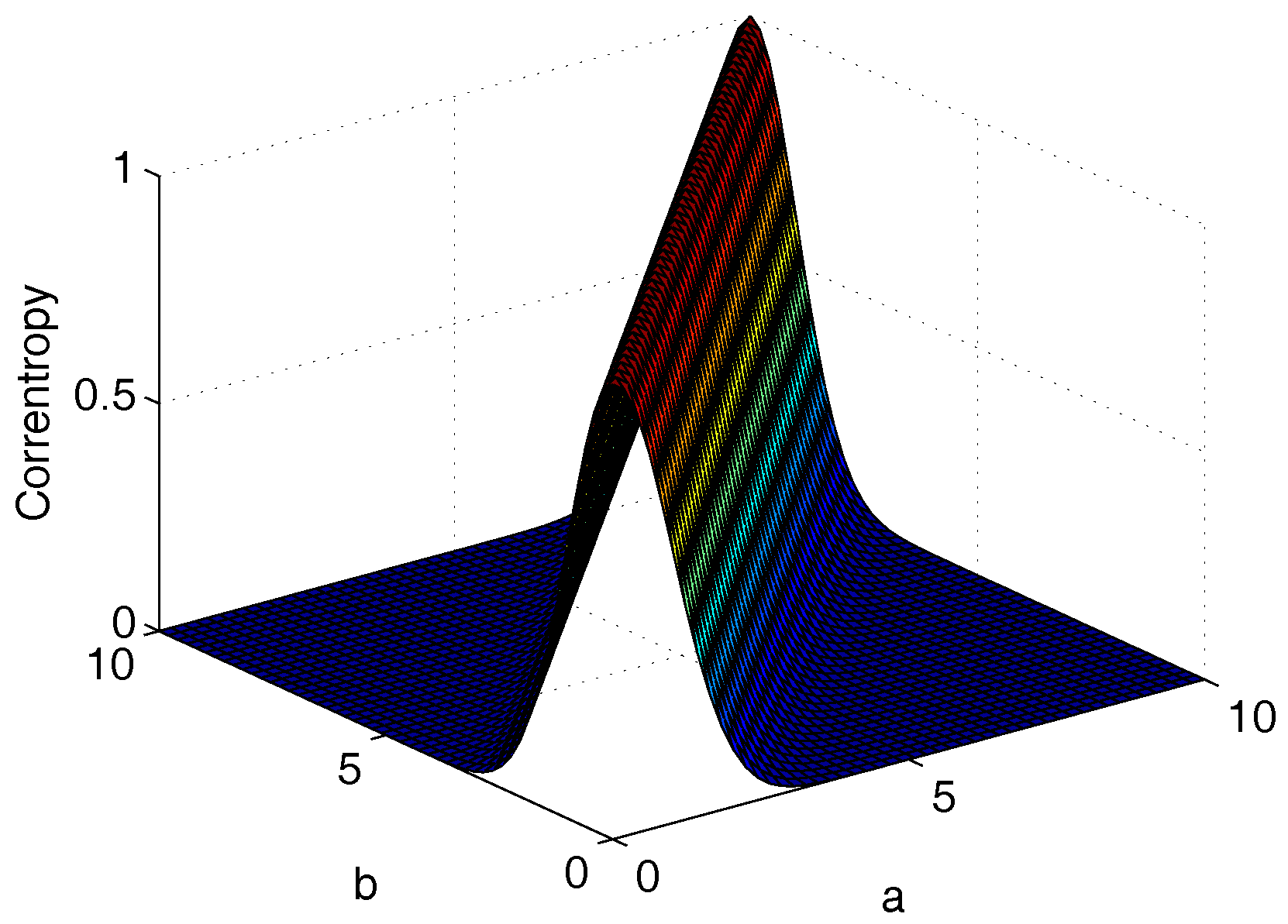
3.2.1. Correntropy

Correntropy [41] defines a metric in the data space and it is directly related to information entropy. It induces a new metric in the sample space that is equivalent to the 2-norm distance [42,43,44]. Given two random variables, $\mathit{A},\mathit{B}\in \mathbb{R}$ with the joint probability density function (PDF) $p\left(a,b\right)$. Then, the definition of the correntropy between two random variables is as follows:

Definition 1.

Correntropy is a generalized similarity measure between two arbitrary scalar random variables $\mathit{A}$ and $\mathit{B}$ defined by

$$\begin{array}{c}{C}_{\lambda }\left(\mathit{A},\mathit{B}\right)=\mathrm{E}\left[\kappa \left(\mathit{A},\mathit{B}\right)\right]=\int \int {\kappa }_{\lambda }\left(a,b\right)p\left(a,b\right)\mathrm{d}a\mathrm{d}b,\end{array}$$

(23)

where E is the expectation and ${\kappa }_{\lambda }$ (_▪,_▪) is any continuous positive definite kernel function, $\lambda >0$ is the kernel size.

In this paper, the kernel function is chosen as the Gaussian kernel given by

$$\begin{array}{c}{\kappa }_{\lambda }\left(a,b\right)={\mathrm{G}}_{\lambda }\left(e\right)=exp\left(-\frac{e^2}{2{\lambda }^2}\right),\end{array}$$

(24)

where $e=a-b$.

In practice, the joint PDF $p\left(a,b\right)$ is unknown and a finite number of sample data are available. Therefore, the correntropy can be estimated by the sample mean estimator:

$$\begin{array}{c}{\widehat{C}}_{\lambda }\left(\mathit{A},\mathit{B}\right)=\frac{1}{N}\sum _{i=1}^N{G}_{\lambda }\left(e_i\right),\end{array}$$

(25)

where $e_i=a_i-b_i$, with ${\left\{a_i,b_i\right\}}_{i=1}^N$ being N samples drawn from $p\left(a,b\right)$.

When $\lambda =1$, $a_i\in \left[0,10\right]$, $b_i\in \left[0,10\right]$ and the samples number is 50, the correntropy can be shown as Figure 1:

As can be seen from Figure 1, the correntropy can be used as a similarity measure in the joint space. In addition, when $a_i=b_i$, the correntropy reaches the maximum value. The cost function that incarnates the maximum correntropy criterion (MCC) is:

$$\begin{array}{c}{J}_{MCC}=max\sum _{i=1}^N{G}_{\lambda }\left(e_i\right).\end{array}$$

(26)

MCC has a probabilistic meaning of maximizing the error probability density at the origin [41], and it has the advantages that it is a local criterion of similarity and it is very useful for non-Gaussian noise [45]. In other words, compared with the mean square error (MSE), MCC is local along the bisector of the joint space, which means that the maximum correntropy value is mainly decided by the kernel function along the line $\mathit{A}=\mathit{B}$ [46].

3.2.2. Maximum Correntropy Criterion Kalman Filter Algorithm

Similar to Equation (19), the maximum correntropy criterion Kalman filter (MCCKF) is designed based on the MCC theory. We have the correntropy-based objective function:

$$\begin{array}{c}{\widehat{\mathit{X}}}_k=arg\underset{{\mathit{X}}_k}{max}J\left({\mathit{X}}_k\right),\end{array}$$

(27)

where

$$\begin{array}{c}J\left({\mathit{X}}_k\right)=G_{\lambda }\left({∥{\mathit{X}}_k-{\mathbf{\Phi }}_{k|k-1}{\widehat{\mathit{X}}}_{k-1}∥}_{{\mathit{P}}_{k|k-1}^{-1}}\right)+G_{\lambda }\left({∥{\mathit{Z}}_k-{\mathit{H}}_k{\mathit{X}}_k∥}_{{\mathit{R}}_k^{-1}}\right),\end{array}$$

(28)

where ${\mathit{R}}_k^{-1}$ and ${\mathit{P}}_{k|k-1}^{-1}$ are chosen as the weighting matrices.

The derivative of Equation (28) with respect to ${\mathit{X}}_k$ is:

$$\begin{array}{c}\begin{array}{c}{G}_{\lambda }\left({∥{\mathit{X}}_k-{\mathbf{\Phi }}_{k|k-1}{\widehat{\mathit{X}}}_{k-1}∥}_{{\mathit{P}}_{k|k-1}^{-1}}\right){\mathit{P}}_{k|k-1}^{-1}\left({\mathit{X}}_k-{\mathbf{\Phi }}_{k|k-1}{\widehat{\mathit{X}}}_{k-1}\right)\hfill \\ -G_{\lambda }\left({∥{\mathit{Z}}_k-{\mathit{H}}_k{\mathit{X}}_k∥}_{{\mathit{R}}_k^{-1}}\right){\mathit{H}}_k^{\mathrm{T}}{\mathit{R}}_k^{-1}\left({\mathit{Z}}_k-{\mathit{H}}_k{\mathit{X}}_k\right)=0.\hfill \end{array}\end{array}$$

(29)

Therefore, ${\widehat{\mathit{X}}}_k$ is the solution of Equation (29). Let

$$\begin{array}{c}{\mathit{P}}_{k|k-1}^{-1}\left({\widehat{\mathit{X}}}_k-{\mathbf{\Phi }}_{k|k-1}{\widehat{\mathit{X}}}_{k-1}\right)=L_k{\mathit{H}}_k^{\mathrm{T}}{\mathit{R}}_k^{-1}\left({\mathit{Z}}_k-{\mathit{H}}_k{\widehat{\mathit{X}}}_k\right),\end{array}$$

(30)

where $L_k=\frac{G_{\lambda }\left({∥{\mathit{Z}}_k-{\mathit{H}}_k{\widehat{\mathit{X}}}_k∥}_{{\mathit{R}}_k^{-1}}\right)}{G_{\lambda }\left({∥{\widehat{\mathit{X}}}_k-{\mathbf{\Phi }}_{k|k-1}{\widehat{\mathit{X}}}_{k-1}∥}_{{\mathit{P}}_{k|k-1}^{-1}}\right)}$. Then, $\left(L_k{\mathit{H}}_k^{\mathrm{T}}{\mathit{R}}_k^{-1}{\mathit{H}}_k{\widehat{\mathit{X}}}_{k|k-1}\right)$ is added and subtracted on the right-hand side of Equation (30) to obtain

$$\begin{array}{c}\begin{array}{c}\begin{array}{c}{\mathit{P}}_{k|k-1}^{-1}\left({\widehat{\mathit{X}}}_k-{\mathbf{\Phi }}_{k|k-1}{\widehat{\mathit{X}}}_{k-1}\right)=\hfill \\ L_k{\mathit{H}}_k^{\mathrm{T}}{\mathit{R}}_k^{-1}\left({\mathit{Z}}_k-{\mathit{H}}_k{\widehat{\mathit{X}}}_k\right)+L_k{\mathit{H}}_k^{\mathrm{T}}{\mathit{R}}_k^{-1}{\mathit{H}}_k{\widehat{\mathit{X}}}_{k|k-1}-L_k{\mathit{H}}_k^{\mathrm{T}}{\mathit{R}}_k^{-1}{\mathit{H}}_k{\widehat{\mathit{X}}}_{k|k-1},\hfill \end{array}\hfill \end{array}\end{array}$$

(31)

$$\begin{array}{c}\begin{array}{c}{\mathit{P}}_{k|k-1}^{-1}{\widehat{\mathit{X}}}_k-{\mathit{P}}_{k|k-1}^{-1}{\mathbf{\Phi }}_{k|k-1}{\widehat{\mathit{X}}}_{k-1}={\mathit{P}}_{k|k-1}^{-1}{\widehat{\mathit{X}}}_k-{\mathit{P}}_{k|k-1}^{-1}{\widehat{\mathit{X}}}_{k|k-1}=\hfill \\ L_k{\mathit{H}}_k^{\mathrm{T}}{\mathit{R}}_k^{-1}{\mathit{Z}}_k-L_k{\mathit{H}}_k^{\mathrm{T}}{\mathit{R}}_k^{-1}{\mathit{H}}_k{\widehat{\mathit{X}}}_k\hfill \\ +L_k{\mathit{H}}_k^{\mathrm{T}}{\mathit{R}}_k^{-1}{\mathit{H}}_k{\widehat{\mathit{X}}}_{k|k-1}-L_k{\mathit{H}}_k^{\mathrm{T}}{\mathit{R}}_k^{-1}{\mathit{H}}_k{\widehat{\mathit{X}}}_{k|k-1},\hfill \end{array}\end{array}$$

(32)

$$\begin{array}{c}\begin{array}{c}\left({\mathit{P}}_{k|k-1}^{-1}+L_k{\mathit{H}}_k^{\mathrm{T}}{\mathit{R}}_k^{-1}{\mathit{H}}_k\right){\widehat{\mathit{X}}}_k\hfill \\ ={\mathit{P}}_{k|k-1}^{-1}{\widehat{\mathit{X}}}_{k|k-1}+L_k{\mathit{H}}_k^{\mathrm{T}}{\mathit{R}}_k^{-1}{\mathit{H}}_k{\widehat{\mathit{X}}}_{k|k-1}+L_k{\mathit{H}}_k^{\mathrm{T}}{\mathit{R}}_k^{-1}\left({\mathit{Z}}_k-{\mathit{H}}_k{\widehat{\mathit{X}}}_{k|k-1}\right)\hfill \\ =\left({\mathit{P}}_{k|k-1}^{-1}+L_k{\mathit{H}}_k^{\mathrm{T}}{\mathit{R}}_k^{-1}{\mathit{H}}_k\right){\widehat{\mathit{X}}}_{k|k-1}+L_k{\mathit{H}}_k^{\mathrm{T}}{\mathit{R}}_k^{-1}\left({\mathit{Z}}_k-{\mathit{H}}_k{\widehat{\mathit{X}}}_{k|k-1}\right),\hfill \end{array}\end{array}$$

(33)

$$\begin{array}{c}\begin{array}{cc}\hfill {\widehat{\mathit{X}}}_k& ={\widehat{\mathit{X}}}_{k|k-1}+{\left({\mathit{P}}_{k|k-1}^{-1}+L_k{\mathit{H}}_k^{\mathrm{T}}{\mathit{R}}_k^{-1}{\mathit{H}}_k\right)}^{-1}{L}_k{\mathit{H}}_k^{\mathrm{T}}{\mathit{R}}_k^{-1}\left({\mathit{Z}}_k-{\mathit{H}}_k{\widehat{\mathit{X}}}_{k|k-1}\right)\hfill \\ & ={\widehat{\mathit{X}}}_{k|k-1}+{\mathit{K}}_k\left({\mathit{Z}}_k-{\mathit{H}}_k{\widehat{\mathit{X}}}_{k|k-1}\right).\hfill \end{array}\end{array}$$

(34)

In addition, then the MCCKF algorithm can be derived from Equation (34) as follows:

• State Prediction

  $$\begin{array}{c}{\widehat{\mathit{X}}}_{k|k-1}={\mathbf{\Phi }}_{k|k-1}{\widehat{\mathit{X}}}_{k-1},\end{array}$$

  (35)
• Covariance Prediction

  $$\begin{array}{c}{\mathit{P}}_{k|k-1}={\mathbf{\Phi }}_{k|k-1}{\mathit{P}}_{k-1|k-1}{\mathbf{\Phi }}_{k|k-1}^{\mathrm{T}}+{\mathit{Q}}_k,\end{array}$$

  (36)
• Filter Gain

  $$\begin{array}{c}{\mathit{K}}_k={\left({\mathit{P}}_{k|k-1}^{-1}+L_k{\mathit{H}}_k^{\mathrm{T}}{\mathit{R}}_k^{-1}{\mathit{H}}_k\right)}^{-1}{L}_k{\mathit{H}}_k^{\mathrm{T}}{\mathit{R}}_k^{-1},\end{array}$$

  (37)
• State Update

  $$\begin{array}{c}{\widehat{\mathit{X}}}_k={\widehat{\mathit{X}}}_{k|k-1}+{\mathit{K}}_k\left({\mathit{Z}}_k-{\mathit{H}}_k{\widehat{\mathit{X}}}_{k|k-1}\right),\end{array}$$

  (38)
• Covariance Update

  $$\begin{array}{c}{\mathit{P}}_{k|k}=\left(\mathit{I}-{\mathit{K}}_k{\mathit{H}}_k\right){\mathit{P}}_{k|k-1}{\left(\mathit{I}-{\mathit{K}}_k{\mathit{H}}_k\right)}^{\mathrm{T}}+{\mathit{K}}_k{\mathit{R}}_k{\mathit{K}}_k^{\mathrm{T}}.\end{array}$$

  (39)

3.3. Robustness of MCCKF

The advantage of MCCKF is that the algorithm uses a method similar to Huber-based filter (HF) [47], which can resist the non-Gaussian noises because the robust function of HF does not increase rapidly as the estimate residual grows. Next, the algorithm robustness is analyzed with the influence function [48] in theory and is compared with HF through the weighting function.

HF is achieved by introducing the concept of the robustness in the maximum likelihood as proposed by Huber [47]. Recall that the maximum likelihood estimator is from a data observation $\mathit{Z}=\left\{z_1,\cdots ,z_N\right\}$, a state variable $\mathit{X}=\left\{x_1,\cdots ,x_N\right\}$. Assuming that $\mathbf{e}=\mathit{Z}-\mathit{HX}$ obeys the distribution and $p\left(\mathbf{e};\mathit{X}\right)$ is known except for the parameters $\mathit{X}$, the MLE of $\mathit{X}$ can be written as

$$\begin{array}{c}{\widehat{\mathit{X}}}_{MLE}=arg\underset{\mathit{X}}{max}p\left(e_1,\cdots ,e_N;\mathit{X}\right).\end{array}$$

(40)

If $e_1,\cdots ,e_N$ are i.i.d. observations, it can be rewritten as

$$\begin{array}{c}\begin{array}{cc}\hfill {\widehat{\mathit{X}}}_{MLE}& =arg\underset{\mathit{X}}{max}{\displaystyle \prod _{i=1}^N}p\left(e_i;\mathit{X}\right)=arg\underset{\mathit{X}}{max}{\displaystyle \sum _{i=1}^N}lnp\left(e_i;\mathit{X}\right)\hfill \\ & =arg\underset{\mathit{X}}{min}{\displaystyle \sum _{i=1}^N}\left(-lnp\left(e_i;\mathit{X}\right)\right).\hfill \end{array}\end{array}$$

(41)

Assume that $\rho$ is a function that satisfies $\rho \left(e_i;\mathit{X}\right)=a\left(-lnp\left(e_i;\mathit{X}\right)\right)+b$, where $a>0$ and b is irrelevant to $\mathit{X}$. Therefore, ${\widehat{\mathit{X}}}_{MLE}$ satisfies

$$\begin{array}{c}\sum _{i=1}^N\rho \left(e_i;\mathit{X}\right)=\sum _{i=1}^N\rho \left(z_i-\mathit{H}{x}_i\right)=\underset{\mathit{X}}{min}\sum _{i=1}^N\rho \left(e_i;\mathit{X}\right).\end{array}$$

(42)

For some parametric models, if the errors in the target track model are assumed as purely stochastic white and follow a Gaussian distribution with zero mean and constant variance ${\sigma }^2$, then the maximum likelihood estimation can be solved. However, in practice, the measurement equipment are affected by external environment or break down. Therefore, the measurement outliers cannot be avoided. In addition, some errors obey the Gaussian distributions with different mean values and variances with most errors. For example, for one error, its distribution can be described as follows:

$$\begin{array}{c}F\left(e_i;\mathit{X}\right)=\left(1-\upsilon \right)F_0\left(e_i;\mathit{X}\right)+\upsilon F_c\left(e_i;\mathit{X}\right),\end{array}$$

(43)

where $F$ (_▪) denotes the mixture distribution, $F_0$ (_▪) is a known normal distribution, $F_c$ (_▪) is a contaminated distribution that is unknown, $\upsilon$ denotes the contamination ratio [49], which is usually much smaller than 1. For Equation (43), it is impractical to solve the maximum likelihood estimation by Equation (42).

For this problem, Huber promoted that $\rho$ can change freely within limits. The method to solve Equation (42) is called M-estimation.

Huber defined the M-estimators as a generalization of maximum likelihood as

$$\begin{array}{c}\underset{\mathit{X}}{min}\sum _{i=1}^N\rho \left(e_i;\mathit{X}\right)or\sum _{i=1}^N\phi \left(e_i;\mathit{X}\right)=0with\phi \left(e_i;\mathit{X}\right)=\frac{d\rho \left(e_i;\mathit{X}\right)}{d{e}_i},\end{array}$$

(44)

where $\rho \left(\mathit{e}\right)$ is called the cost or penalty function [48] and must obey the properties:

$$\begin{array}{c}\begin{array}{c}1.\rho \left(e\right)\ge 0\hfill \\ 2.\rho \left(0\right)=0\hfill \\ 3.\rho \left(e\right)=\rho \left(-e\right)\hfill \\ 4.\rho \left(e_i\right)\ge \rho \left(e_j\right),\left|e_i\right|>\left|e_j\right|.\hfill \end{array}\end{array}$$

(45)

Let

$$\begin{array}{c}{\rho }_{MCC}\left(e_i\right)=\left(1-exp\left(-{e_i}^2/2{\lambda }^2\right)\right)/\phantom{\left(1-exp\left(-{e_i}^2/2{\lambda }^2\right)\right)\sqrt{2\pi }}\sqrt{2\pi }\lambda .\end{array}$$

(46)

It is trivial to check that it obeys the properties of Equation (45). Furthermore,

$$\begin{array}{c}\begin{array}{c}min{\displaystyle \sum _{i=1}^N}{\rho }_{MCC}\left(e_i\right)\hfill \\ =min{\displaystyle \sum _{i=1}^N}\left(1-exp\left(-{e_i}^2/2{\lambda }^2\right)\right)/\phantom{\left(1-exp\left(-{e_i}^2/2{\lambda }^2\right)\right)\sqrt{2\pi }}\sqrt{2\pi }\lambda \hfill \\ \iff max{\displaystyle \sum _{i=1}^N}exp\left(-{e_i}^2/2{\lambda }^2\right)/\phantom{exp\left(-{e_i}^2/2{\lambda }^2\right)\sqrt{2\pi }}\sqrt{2\pi }\lambda \hfill \\ =max{\displaystyle \sum _{i=1}^N}{G}_{\lambda }\left(e_i\right).\hfill \end{array}\end{array}$$

(47)

In other words, there is a connection with MCC and Equation (46) [50,51]:

$$\underset{\mathit{X}}{min}\sum _{i=1}^N{\rho }_{MCC}\left(e_i\right)isequivalenttoMCC=\underset{\mathit{X}}{max}\sum _{i=1}^N{G}_{\lambda }\left(e_i\right).$$

Considering the M-estimation problem, the weighting function ${\psi }_{MCC}\left(e_i\right)$ is defined by

$$\begin{array}{c}{\psi }_{MCC}\left(e_i\right)=\frac{{{\rho }_{MCC}}^{\prime }\left(e_i\right)}{e_i},\end{array}$$

(48)

where ${{\rho }_{MCC}}^{\prime }\left(e_i\right)=\frac{d{\rho }_{MCC}\left(e_i\right)}{d{e}_i}$. Therefore,

$$\begin{array}{c}{\psi }_{MCC}\left(e_i\right)=exp\left(-{e_i}^2/2{\lambda }^2\right)/\phantom{exp\left(-{e_i}^2/2{\lambda }^2\right)\sqrt{2\pi }}\sqrt{2\pi }{\lambda }^3.\end{array}$$

(49)

Based on the penalty function and the weighting function above, we will analyze the robustness with influence function and compare it with Huber-filter to prove the superiority of MCCKF.

3.3.1. Influence Function of MCCKF

Influence function (IF) is a quantitative measure to evaluate the robustness of Kalman filter [52]. The conventional definition of IF is defined as:

Definition 2.

For any $l\in \mathbb{R}$, $\mathbb{R}$ is the real set, $\delta l$ is the probability distribution that is degraded in l and the mixture distribution is:

$$\begin{array}{c}F=\left(1-\upsilon \right)F_0+\upsilon \delta l\left(0\le \upsilon \le 1\right),\end{array}$$

(50)

where $F_0$ is the main distribution, and υ is the contamination ratio, and then if the limit

$$IF\left(l;F_0,T\right)=\underset{\upsilon \to 0}{lim}\frac{T\left(F\right)-T\left(F_0\right)}{\upsilon }={\left.\frac{dT\left(F\right)}{d\upsilon }\right|}_{\upsilon =0}$$

(51)

exists, where $T\left(F\right)$ is one functional expression of the distribution function F, then $IF\left(l;F_0,T\right)$ is called the influence function about $T\left(F\right)$.

The traditional definition of IF describes the relative influence of a contaminated measurement on functional T. The smaller the IF is, the more insensitive the reflection on the contaminated measurement of T is. In other words, for the fixed distribution F, the change of IF reflects the different influences on different measurements. Thus, it can effectively reflect the robustness of Kalman filter.

However, the traditional form of IF is sometimes complex to analyze the performance of Kalman filter. For analyzing the robustness of Kalman filter more clearly, Chang [48] derived a new form of the influence function. According to Equation (16), construct a following pseudo-measurement

$${\mathcal{Z}}_k=\left[\begin{array}{c}{\widehat{\mathit{X}}}_{k|k-1}\\ {\mathit{Z}}_k\end{array}\right]=\left[\begin{array}{c}{\mathit{X}}_k\\ {\mathit{H}}_k{\mathit{X}}_k\end{array}\right]+\left[\begin{array}{c}\delta {\widehat{\mathit{X}}}_{k|k-1}\\ {\mathit{V}}_k\end{array}\right]={\mathcal{H}}_k{\mathit{X}}_k+{\mathcal{V}}_k$$

(52)

with

$$\mathrm{E}\left({\mathcal{V}}_k\right)=0,\mathrm{E}\left[\left({\mathcal{V}}_k\right){\left({\mathcal{V}}_k\right)}^{\mathrm{T}}\right]={\mathcal{R}}_k={\mathit{P}}_{{\mathcal{V}}_k}=\left[\begin{array}{cc}{\mathit{P}}_{{\widehat{\mathit{X}}}_{k|k-1},{\widehat{\mathit{X}}}_{k|k-1}}& \mathit{O}\\ \mathit{O}& {\mathit{R}}_k\end{array}\right],$$

(53)

with ${\mathcal{Z}}_k$ as the measurement and ${\mathit{X}}_k$ as the parameter to be estimated. Equation (52) is exactly a classic linear regression problem with the known statistics of the measurements, which can be solved using the weighted least square methods as

$${\widehat{\mathit{X}}}_k={\left({\mathcal{H}}_k^{\mathrm{T}}{\mathcal{R}}_k^{-1}{\mathcal{H}}_k\right)}^{-1}{\mathcal{H}}_k^{\mathrm{T}}{\mathcal{R}}_k^{-1}{\mathcal{Z}}_k,$$

(54)

$${\mathit{P}}_{{\widehat{\mathit{X}}}_k{\widehat{\mathit{X}}}_k}={\left({\mathcal{H}}_k^{\mathrm{T}}{\mathcal{R}}_k^{-1}{\mathcal{H}}_k\right)}^{-1}.$$

(55)

Define

$${\stackrel{⌣}{\mathcal{Z}}}_k={\mathcal{R}}_k^{-1/2}{\mathcal{Z}}_k,$$

(56)

$${\stackrel{⌣}{\mathcal{H}}}_k={\mathcal{R}}_k^{-1/2}{\mathcal{H}}_k,$$

(57)

$${\stackrel{⌣}{\mathcal{V}}}_k={\mathcal{R}}_k^{-1/2}{\mathcal{V}}_k,$$

(58)

where ${\mathcal{R}}_k^{-1/2}={\left({\mathcal{R}}_k^{1/2}\right)}^{-1}$ and ${\mathcal{R}}_k^{1/2}{\left({\mathcal{R}}_k^{1/2}\right)}^{\mathrm{T}}={\mathcal{R}}_k$. Then,

$${\stackrel{⌣}{\mathcal{Z}}}_k={\stackrel{⌣}{\mathcal{H}}}_k{\mathit{X}}_k+{\stackrel{⌣}{\mathcal{V}}}_k$$

(59)

$$\mathrm{E}\left[{\stackrel{⌣}{\mathcal{V}}}_k\right]=0,{\mathit{P}}_{{\stackrel{⌣}{\mathcal{V}}}_k,{\stackrel{⌣}{\mathcal{V}}}_k}=\mathit{I}$$

(60)

For the sake of brevity, the subscript k is omitted and let $m=n_x+n_y$ in the sequel, where $n_x$, $n_y$ denotes the dimension of the state vector and the measurement vector. Find the ML solution to Equation (59) through maximizing the following likelihood function

$$L\left(\widehat{\mathit{X}},\mathit{r}\right)=\prod _{j=1}^{m}F\left({\mathit{r}}_j\right),$$

(61)

where $\mathit{r}={\stackrel{⌣}{\mathcal{Z}}}_k-{\stackrel{⌣}{\mathcal{H}}}_k{\hat{\mathit{X}}}_k, F$ (_▪) denotes the probability distribution. Similar to Equation (41), Equation (61) is equal to the following form:

$$\begin{array}{c}\hfill J\left(\widehat{\mathit{X}},\mathit{r}\right)=-ln\left[L\left(\widehat{\mathit{X}},\mathit{r}\right)\right]=\sum _{i=1}^m-lnp\left(r_j\right)=\sum _{i=1}^m\rho \left(r_i\right),\end{array}$$

(62)

where $\rho$ (_▪) is the cost or penalty function. Then, a necessary condition for theminimizer in Equation (62) is

$$\sum _{i=1}^m{\rho }^{\prime }\left(r_i\right)\frac{\partial r_i}{\partial \widehat{\mathit{X}}}=\sum _{i=1}^m\varphi \left(r_i\right)\frac{\partial r_i}{\partial \widehat{\mathit{X}}}=\sum _{i=1}^m{\varphi \left(r_i\right)\stackrel{⌣}{h}}_i^{\mathrm{T}}=0,$$

(63)

where

$$\varphi \left({}_{\blacksquare }\right)={\rho }^{\prime }\left({}_{\blacksquare }\right)$$

(64)

and ${\stackrel{⌣}{h}}_i$ is the corresponding column vector of ${\stackrel{⌣}{\mathcal{H}}}^{\mathrm{T}}$ (the measurement matrix). By taking transpose, Equation (63) is equivalent to

$$\sum _{i=1}^m\varphi \left(r_i\right){\stackrel{⌣}{h}}_i=0.$$

(65)

Define an estimator as $\mathcal{E}\left(F\right)$ explicating that it is a functional of the distribution F. Then, based on the description above, the new form of IF for the distribution Equation (43) is as follows:

$$IF\left(\stackrel{⌣}{h},F_0,\mathcal{E}\right)=\underset{\upsilon \to 0}{lim}\frac{\mathcal{E}\left(F_0\left(1-\upsilon \right)+F_c\upsilon \right)-\mathcal{E}\left(F_0\right)}{\upsilon }={\left.\frac{\partial \mathcal{E}\left(F_{\upsilon }\right)}{\partial \upsilon }\right|}_{\upsilon =0},$$

(66)

where $\stackrel{⌣}{h}$ is the generalization of ${\stackrel{⌣}{h}}_j$ representing the corresponding column vector of ${\stackrel{⌣}{\mathcal{H}}}^{\mathrm{T}}$, $\upsilon \downarrow 0$ stands for the limit from right. It evaluates the infinitesimal influence on the estimator $\mathcal{E}$ of any single measurement whose residual is r, which comes from the neighborhood of the distribution $F_0$ through the designing matrix ${\stackrel{⌣}{h}}^{\mathrm{T}}$. Let the method of estimating $\hat{\mathit{X}}$ for the m-sample data be denoted as ${\mathcal{E}}_m$. Then, according to the relation between $\hat{\mathit{X}}$ and r, Chang [48] transformed the definition of IF in another form to obtain the IF of ${\mathcal{E}}_m$. It is derived in Ref. [48] in detail. The IF to assess the influence of one of the m elements of the pseudo-measurement vector in Equation (59) is defined as:

$$\begin{array}{c}\hfill IF\left(r,\stackrel{⌣}{h},F_0,\mathcal{E}\right)=\frac{\varphi \left(r_j\right)}{E_{F_0}\left[{\varphi }^{\prime }\left(r\right)\right]}{\left({\stackrel{⌣}{\mathcal{H}}}^{\mathrm{T}}\stackrel{⌣}{\mathcal{H}}\right)}^{-1}\end{array}{\stackrel{⌣}{h}}_j,j=1,2,\cdots ,m,$$

(67)

where $r_j$ is the j-th element of r.

Three requirements about the IF are needed for an estimator to be infinitesimally robust, i.e., boundedness, continuity, and linearity at the center [48].

Next, we will prove that MCCKF satisfies the requirements above.

According to the Equation (46), the estimator of MCCKF with its cost function as

$${\varphi }_{MCC}\left(e\right)={\rho }_{MCC}^{\prime }\left(e\right)=\frac{e}{\sqrt{2\pi }{\lambda }^3}exp\left(-\frac{e^2}{2{\lambda }^2}\right)$$

(68)

and

$${\varphi }_{MCC}^{\prime }\left(e\right)=\frac{1}{\sqrt{2\pi }{\lambda }^3}exp\left(-\frac{e^2}{2{\lambda }^2}\right)-\frac{e^2}{\sqrt{2\pi }{\lambda }^5}exp\left(-\frac{e^2}{2{\lambda }^2}\right).$$

(69)

Then,

$$\begin{array}{cc}\hfill E_{F_0}\left[{{\varphi }^{\prime }}_{MCC}\left(e\right)\right]& ={\int }_{-\infty }^{+\infty }{{\varphi }^{\prime }}_{MCC}\left(e\right)d{F}_0\hfill \\ & =\frac{\left({\lambda }^2+{\sigma }^2\right)-\sqrt{2\pi }}{\sqrt{2\pi }{\lambda }^2\left({\lambda }^2+{\sigma }^2\right)\sqrt{{\lambda }^2+{\sigma }^2}},\hfill \end{array}$$

(70)

where $\sigma$ is the standard deviation of distribution $F_0$. Therefore, we have the IF of MCC expressed as:

$$\begin{array}{c}I{F}_{MCC}\left(r,\stackrel{⌣}{h},F_0,\mathcal{E}\right)\hfill \\ =\frac{{\varphi }_{MCC}\left(r_j\right)}{E_{F_0}\left[{{\varphi }^{\prime }}_{MCC}\left(r\right)\right]}{\left({\stackrel{⌣}{\mathcal{H}}}^{\mathrm{T}}\stackrel{⌣}{\mathcal{H}}\right)}^{-1}{\stackrel{⌣}{h}}_j,\hfill \end{array}$$

(71)

where $E_{F_0}\left[{{\varphi }^{\prime }}_{MCC}\left(r\right)\right]$ is a constant (proved in Equation (70)) and ${\left({\mathcal{H}}^{\mathrm{T}}\mathcal{H}\right)}^{-1}{h}_j$ is a known constant matrix. It is trivial to check that the IF in Equation (71) satisfies continuity and linearity at the center. Next, we will prove the boundedness of Equation (71).

According to the statement above, the boundedness of IF depends on ${\varphi }_{MCC}\left(r_j\right)$.

Remark 1.

${\varphi }_{MCC}\left(r\right)$ is a bounded function in the interval $\left(-\infty ,+\infty \right)$.

Proof. 

$$\begin{array}{cc}\hfill {\varphi }_{MCC}\left(r\right)& =\frac{r}{\sqrt{2\pi }{\lambda }^3}exp\left(-\frac{r^2}{2{\lambda }^2}\right)\hfill \\ & =\frac{r}{\sqrt{2\pi }{\lambda }^3}/\phantom{\frac{r}{\sqrt{2\pi }{\lambda }^3}exp\left(\frac{r^2}{2{\lambda }^2}\right)}exp\left(\frac{r^2}{2{\lambda }^2}\right).\hfill \end{array}$$

(72)

It is evident that ${\varphi }_{MCC}\left(r\right)$ is a continuous function, so it satisfies the boundedness in any closed intervals. Furthermore, it is an odd function.

• Fix $\epsilon >0$, and ${\varphi }_{MCC}\left(r\right)$ is bounded in the interval $\left[-\epsilon ,\epsilon \right]$.
• In the interval $\left[\epsilon ,+\infty \right)$, according to the L’Hospital’s rule [53], Equation (72) can be transformed as:

  $$\begin{array}{c}\underset{r\to \infty }{lim}{\varphi }_{MCC}\left(r\right)\hfill \\ =\underset{r\to \infty }{lim}\frac{1}{\sqrt{2\pi }{\lambda }^3}/\phantom{\frac{1}{\sqrt{2\pi }{\lambda }^3}\sqrt{2\pi }\lambda rexp\left(\frac{r^2}{2{\lambda }^2}\right)}\sqrt{2\pi }\lambda rexp\left(\frac{r^2}{2{\lambda }^2}\right)\hfill \\ =0.\hfill \end{array}$$

  (73)

Therefore, ${\varphi }_{MCC}\left(r\right)$ is bounded in $\left[\epsilon ,+\infty \right)$. According to the characteristic of the odd function, it is also bounded in $\left(-\infty ,-\epsilon \right]$. ☐

Hence, the IF of MCCKF satisfies all three of the requirements of a robust estimator, i.e., boundedness, continuity, and linearity at the center.

HF is another filter whose robustness is also proved with IF in [48]. Next, we will compare the MCCKF with HF.

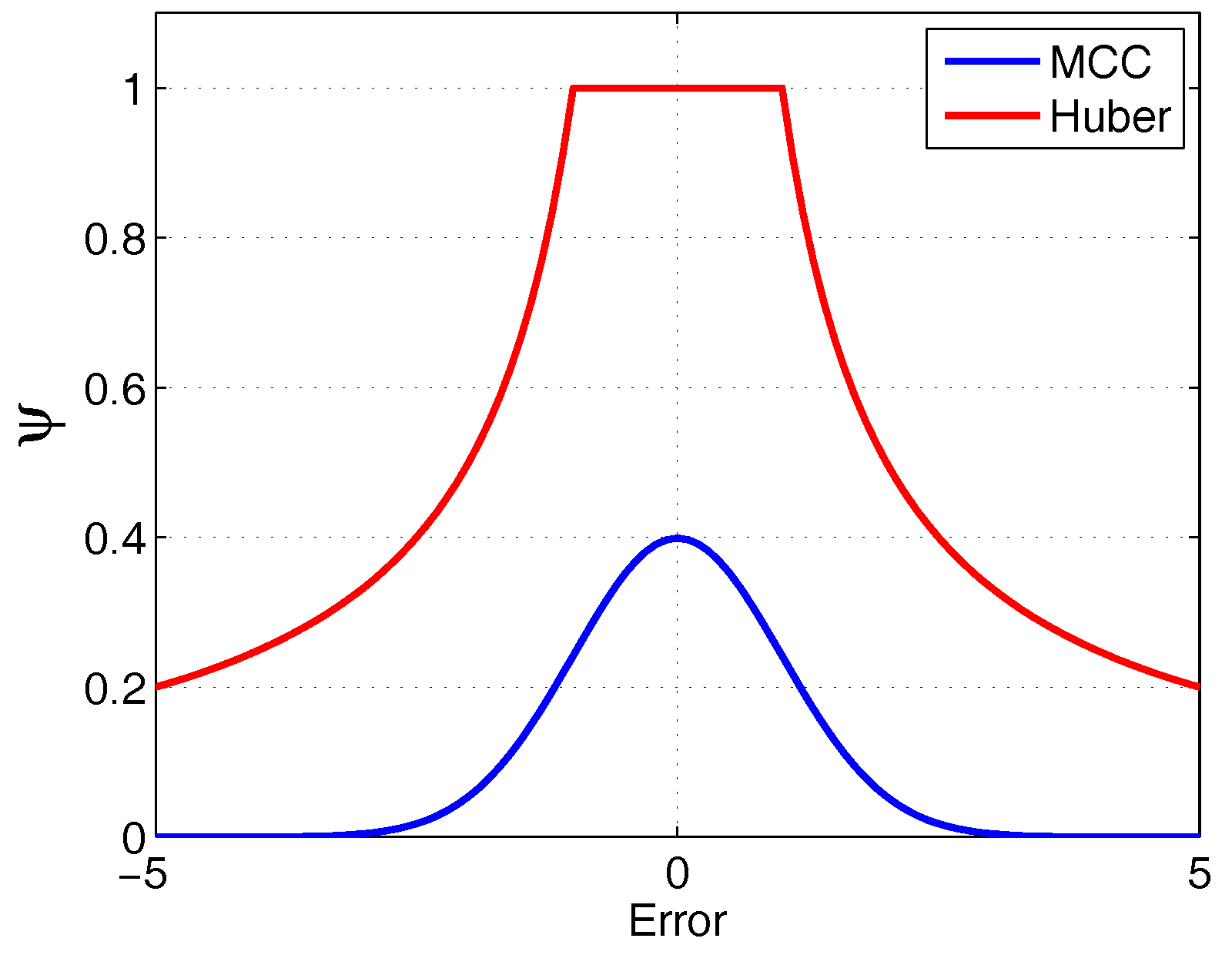
3.3.2. Comparison with Huber Filter

In fact, the Huber-based filter (HF) estimates by minimizing the following cost function [54]

$$\begin{array}{c}\hfill J_{\mathrm{HF}}=min\left(\sum _{i=1}^N{\rho }_{\mathrm{HF}}\left(e_i\right)\right),\end{array}$$

(74)

where ${\rho }_{\mathrm{HF}}$ (_▪) is the designed robust function that is bounded and convex. In other words, a Huber-based filter can resist the non-Gaussian noises because the robust function does not increase rapidly as the estimate residual grows. In addition, the M-estimation function with the expression shown in Equation (74) has several forms. Huber M-estimator [46] is a common one that can be shown as:

$$\begin{array}{c}{\rho }_{\mathrm{Huber}}\left(e_i\right)=\left\{\begin{array}{cc}{e}_i^2/2,& \left|e_i\right|\le \delta ,\\ \delta \left(\left|e_i\right|-\delta /\phantom{\delta 2}2\right),& \left|e_i\right|>\delta .\end{array}\right.\end{array}$$

(75)

Its weighting function is

$$\begin{array}{c}{\psi }_{\mathrm{Huber}}\left(e_i\right)=\left\{\begin{array}{cc}1,& \left|e_i\right|\le \delta ,\\ \delta /\left|e_i\right|,& \left|e_i\right|>\delta ,\end{array}\right.\end{array}$$

(76)

where $\delta$ is the tuning parameter. In a similar manner, Equation (46) can seem like a new $\rho$ (_▪) function in which the kernel size $\lambda$ plays a role similar to $\delta$.

Suppose only one measurement is adopted. Figure 2 shows the ${\psi }_{MCC}$ of the MCC in Equation (49) and ${\psi }_{\mathrm{Huber}}$ in Equation (76) with different errors, in which $\lambda =1$ and $\delta =1$, respectively. The result is also presented in Ref. [46].

The weighting function of MCC and Huber reduces as the error value increases. It means that both methods can reduce the weight of the measurements containing large outliers. However, MCC has a higher speed to zero compared to that of Huber. It means that Huber may employ more large outliers into the estimation process than that of MCC, although their impacts are reduced. In other words, MCC selects those measurements with smaller errors and discards those with a large outlier. MCC can completely remove the inappropriate measurements from the estimation processes and have a better performance. That is, Kalman filter under the MCC can improve the robustness.

From Equation (49), the kernel size $\lambda$ plays an important role in the weighting function. The robustness is decided by the kernel size.

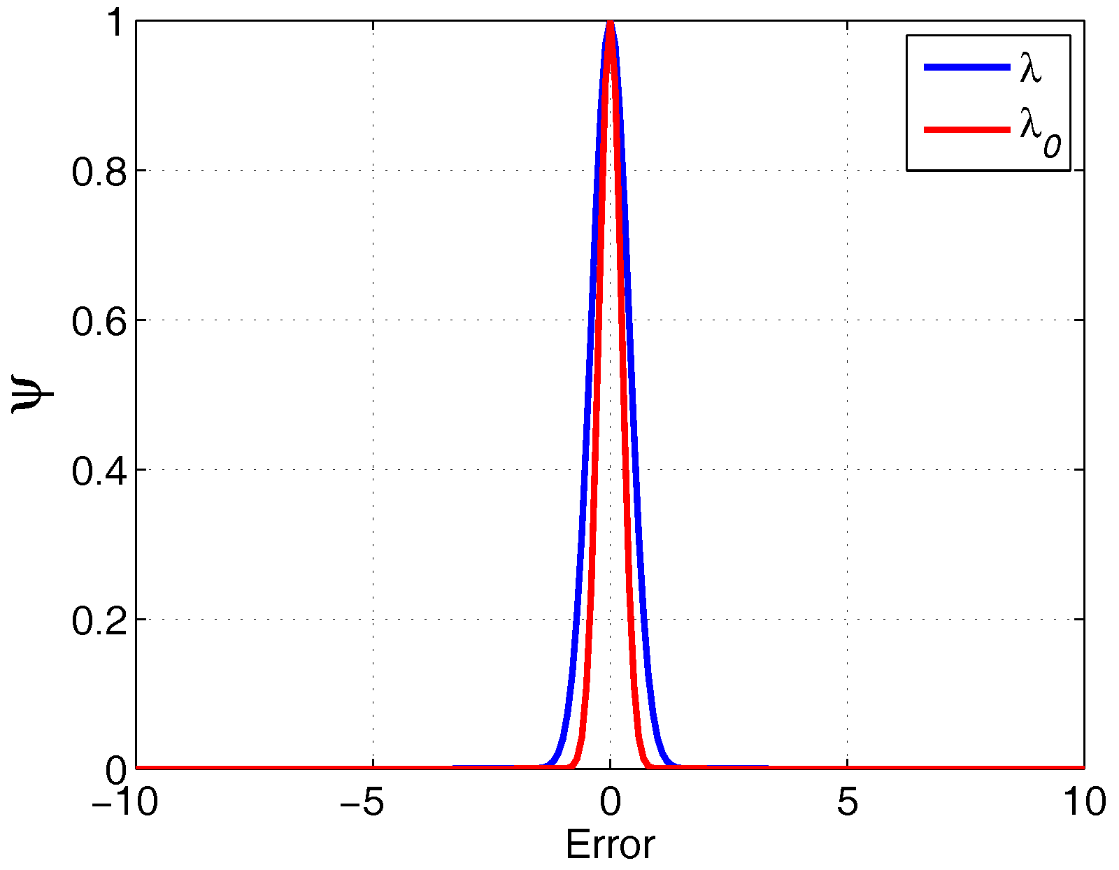
3.4. Kernel Size Selection

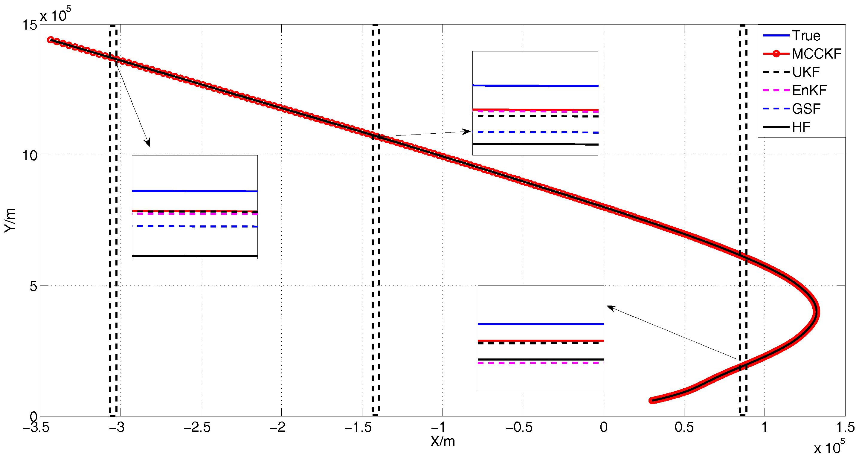
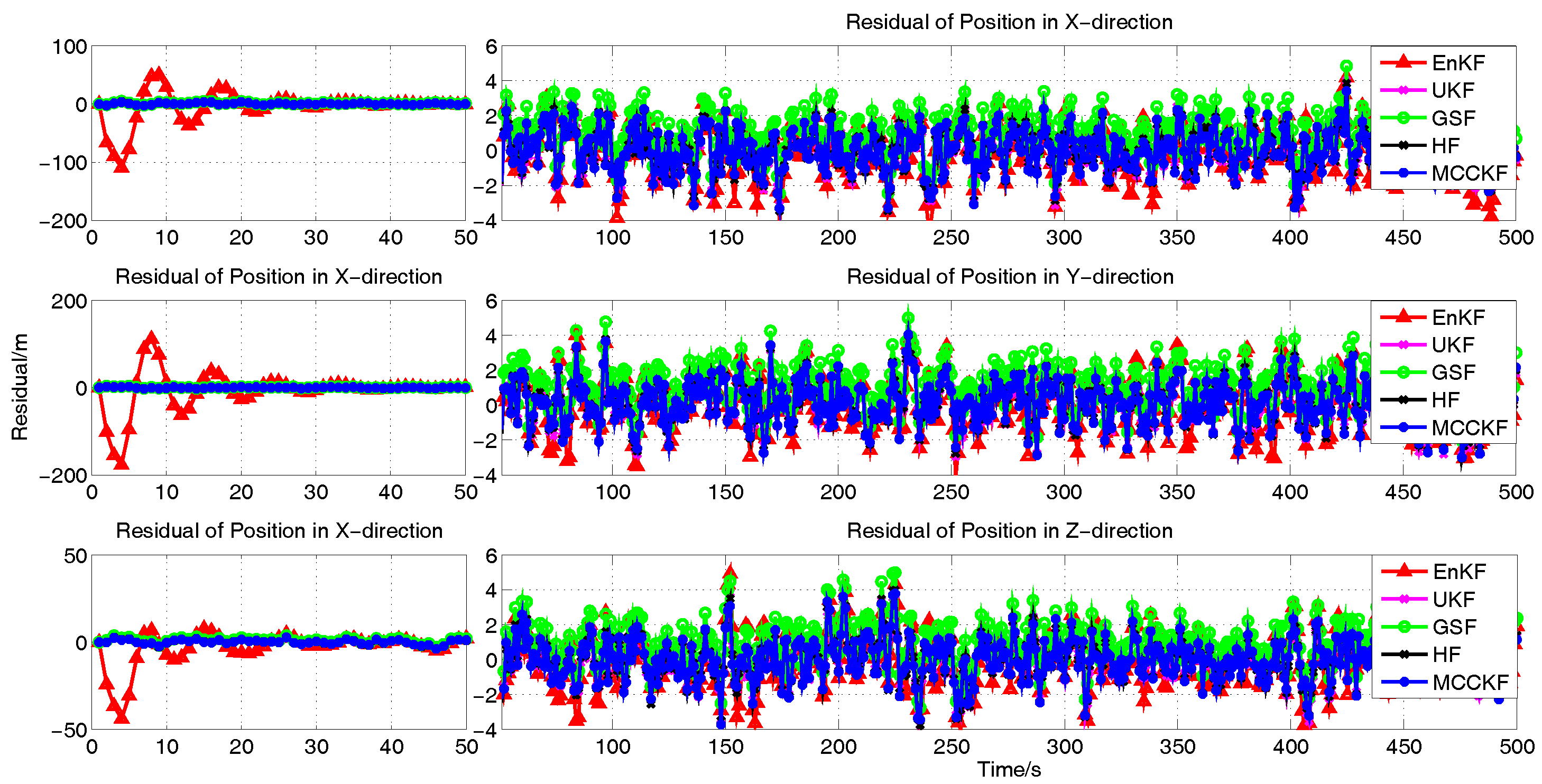
Due to the close relationship between M-estimation and correntropy, choosing an appropriate kernel size in the correntropy criterion becomes practical [54]. In the MCCKF algorithm, or the same input data, different kernel sizes lead to different filter results. If the kernel size is too large, the filter system will degrade into linear regression. If the kernel size is too small, all the data will look distinct and the system cannot infer on unseen samples falling between the training points [55]. Therefore, the kernel size can be adaptively adjusted as other parameters.

There are not many accessible values to the problem for us. However, the measurements, the dynamic system model and the noise parameters are accessible. It is a new thought to make use of this information in the adaption of the kernel size selection. In fact, Cinar et al. [56] has proposed that the best kernel sizes are in the range of the observation errors and half of the cost function has the observation error as the argument and a similar kernel size will get a better result. Based on the idea, he heuristically chose the kernel size at each time instant to be the observation error as shown below:

$$\begin{array}{c}{\lambda }_k=∥{\mathit{Z}}_k-{\mathit{H}}_k{\widehat{\mathit{X}}}_k∥.\end{array}$$

(77)

In this paper, inspired by Equation (77) and combined with the the weighted least square thought, we proposed that the kernel size selection method can be adjusted to

$$\begin{array}{c}{\lambda }_{0_k}=∥{\left({\mathit{Z}}_k-{\mathit{H}}_k{\widehat{\mathit{X}}}_k\right)}^{\mathrm{T}}{\mathit{R}}_k^{-1}\left({\mathit{Z}}_k-{\mathit{H}}_k{\widehat{\mathit{X}}}_k\right)∥.\end{array}$$

(78)

In fact, Equations (77) and (78) reflect the Euclidean distance and the Mahalanobis distance, respectively. Equation (78), which is a novel kernel size selection method proposed in the article, can overcome the influence of the covariance due to the advantages of Mahalanobis distance. It is much more sensitive to the small change of data.

To show the different results of different kernel size, the weights are shown under the different sizes for $\lambda$ in Equation (77) and for ${\lambda }_0$ in Equation (78) as follows.

From Figure 3, ${\lambda }_0$ has a higher speed to zero compared to $\lambda$. ${\lambda }_0$ can employ less outliers than $\lambda$, although both impacts are reduced. Therefore, ${\lambda }_0$ can select the measurements with smaller error and remove more inappropriate measurements from the estimation processes. Therefore, ${\lambda }_0$ is more appropriate than $\lambda$.

4. Simulation

In this section, we mainly demonstrate the performances of the MCCKF in the presence of large outliers and mixture Gaussian noises. The estimation performances are compared based on the following indices:

$$\begin{array}{c}\mathrm{Residual}\left(k\right)={\mathit{X}}_k-{\widehat{\mathit{X}}}_{k|k},k=1,\cdots ,N,\end{array}$$

(79)

$$\begin{array}{c}\mathrm{RMSE}=\frac{1}{M}\sum _{m=1}^M\sqrt{\frac{1}{N}\sum _{i=1}^N{\left({\mathit{X}}_k-{\widehat{\mathit{X}}}_{k|k}\right)}^2},m=1,\cdots ,M,\end{array}$$

(80)

where N is the entire time steps in every Monte Carlo run and M represents the total Monte Carlo runs.

4.1. Simulation Conditions

In this section, simulation experiments are conducted to validate the proposed algorithm for restricting the non-Gaussian noises. The $\alpha$-Jerk model results obtained by the Huber-based filter (HF), ensemble Kalman filter (EnKF), unscented Kalman filter (UKF), Gaussian sum filter (GSF) and maximum correntropy criterion Kalman filter (MCCKF) are compared here.

The target tracking parameters are set as below: time interval is $T=$ 1 s; 500 independent Monte Carlo runs have been conducted, i.e., $M=500$; the measurement noise covariance is $\mathit{R}=diag\left(\left[\begin{array}{ccc}2& 2& 2\end{array}\right]\right)$; the standard deviation of input is ${\sigma }_{\epsilon }=0.7$; the standard deviation of the target ‘jerk’ is ${\sigma }_j=0.2$; and the state vector in three dimensions is

$$\mathit{X}={\left[\begin{array}{cccccccccccc}x& \dot{x}& \ddot{x}& \stackrel{⃛}{x}& y& \dot{y}& \ddot{y}& \stackrel{⃛}{y}& z& \dot{z}& \ddot{z}& \stackrel{⃛}{z}\end{array}\right]}^{\mathrm{T}},$$

which contains the position, the velocity, the acceleration and the ‘jerk’, respectively; the initial true state is

$$\begin{array}{c}x\left(0\right)=30000,\dot{x}\left(0\right)=300,\ddot{x}\left(0\right)=1,\stackrel{⃛}{x}\left(0\right)=0,\hfill \\ y\left(0\right)=60000,\dot{y}\left(0\right)=400,\ddot{y}\left(0\right)=1,\stackrel{⃛}{y}\left(0\right)=0,\hfill \\ z\left(0\right)=90000,\dot{z}\left(0\right)=500,\ddot{z}\left(0\right)=1,\stackrel{⃛}{z}\left(0\right)=0.\hfill \end{array}$$

and the initial covariance matrix of the states are chosen as

$${\mathbf{P}}_{0|0}=diag\left(\left[\begin{array}{cccccccccccc}10000& 1000& 100& 10& 10000& 1000& 100& 10& 10000& 1000& 100& 10\end{array}\right]\right).$$

The initial values in three dimensions are ${\alpha }_x={\alpha }_y={\alpha }_z=0.5$.

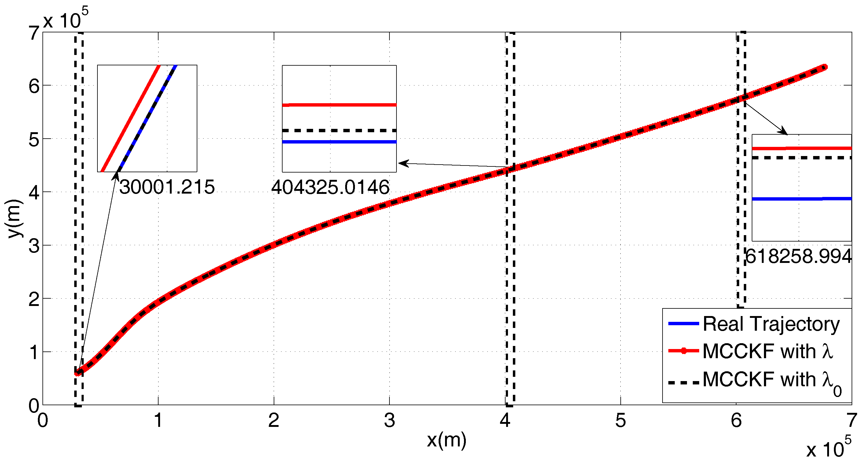
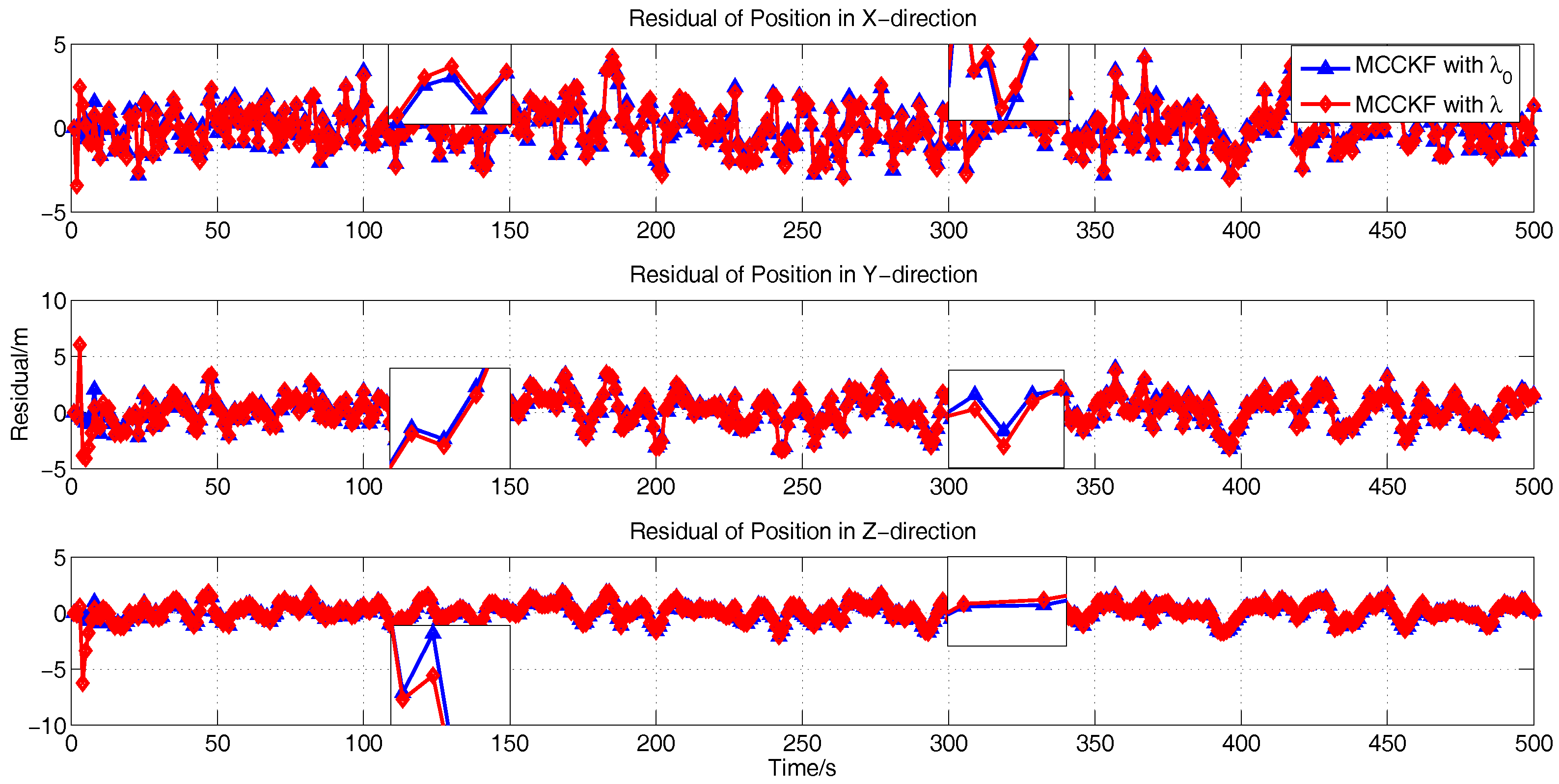
4.2. The Kernel Size Adaptive Method

To choose a better kernel size adaptive method, a simulation is made in this section with Equations (77) and (78), respectively. The simulation conditions are the same as Section 4.1. Figure 4 shows the trajectories in a two-dimensional plane under two kernel size selection methods.

As can be seen from Figure 4 and Figure 5, MCCKF with the new adaptive method ensures a higher accuracy than the other in most time.

Table 1. RMSE of every state variable in the x-direction of two different kernel size selection methods.

	Position (m)	Velocity (m/s)	Accelaration (m/s${}^2$)	Jerk ($\mathbf{m}/{\mathbf{s}}^3$)	$\mathit{\alpha }$
${\mathit{\lambda }}_{\mathbf{0}}$	1.2331	1.3251	0.7766	0.3512	0.2637
$\lambda$	1.2821	1.3590	0.7961	0.3531	0.2764

,

Table 2. RMSE of every state variable in the y-direction of two different kernel size selection methods.

	Position (m)	Velocity (m/s)	Accelaration ($\mathbf{m}/{\mathbf{s}}^2$)	Jerk ($\mathbf{m}/{\mathbf{s}}^3$)	$\mathit{\alpha }$
${\mathit{\lambda }}_{\mathbf{0}}$	1.2325	1.2203	0.6863	0.3248	0.3232
$\lambda$	1.2538	1.2451	0.6905	0.32	0.3232

and

Table 3. RMSE of every state variable in the z-direction of two different kernel size selection methods.

	Position (m)	Velocity (m/s)	Accelaration ($\mathbf{m}/{\mathbf{s}}^2$)	Jerk ($\mathbf{m}/{\mathbf{s}}^3$)	$\mathit{\alpha }$
${\mathit{\lambda }}_{\mathbf{0}}$	1.3477	1.3768	0.8037	0.3581	0.7747
$\lambda$	1.3747	1.3968	0.8256	0.3682	0.7936

show that the newly proposed kenel size selection method in this paper (${\lambda }_0$) indeed has a higher accuracy on the whole.

4.3. The Presence of Gaussian Noise

In this section, we will apply the MCCKF on $\alpha$-jerk model in the presence of Gaussian noises to present the performance of MCCKF. The simulation parameters and the initial state are the same as Section 4.1.

To explain the advantages of MCCKF, we use EnKF, UKF, GSF and HF algorithms to track target with $\alpha$-jerk model compared with MCCKF. Figure 6 demonstrates the real target trajectory and the estimated target trajectories with EnKF, GSF, UKF, HF and MCCKF in a two-dimensional plane. Figure 7 demonstrates the residual defined in Equation (79) with EnKF, UKF, GSF, HF and MCCKF.

Table 4. RMSE of every state variable in the x-direction of EnKF, UKF, GSF, HF and MCCKF algorithms.

	Position (m)	Velocity (m/s)	Accelaration ($\mathbf{m}/{\mathbf{s}}^2$)	Jerk ($\mathbf{m}/{\mathbf{s}}^3$)	$\mathit{\alpha }$
EnKF	7.0350	4.7926	2.3029	0.5543	1.7291
UKF	1.2892	1.3825	0.8940	0.4424	1.6125
GSF	1.5990	1.2220	0.8072	0.4202	1.6125
HF	1.2843	1.2220	0.8072	0.4202	1.6125
MCCKF	1.2901	1.2252	0.8076	0.4201	1.6125

,

Table 5. RMSE of every state variable in the y-direction of EnKF, UKF, GSF, HF and MCCKF algorithms.

	Position (m)	Velocity (m/s)	Accelaration ($\mathbf{m}/\mathbf{s}{}^2$)	Jerk ($\mathbf{m}/\mathbf{s}{}^3$)	$\mathit{\alpha }$
EnKF	3.2812	3.9866	2.1125	0.5019	3.2963
UKF	1.2856	1.5343	0.9418	0.4299	1.1582
GSF	1.5749	1.3181	0.8666	0.4245	1.1582
HF	1.2695	1.3181	0.8666	0.4245	1.1582
MCCKF	1.2695	1.3195	0.8685	0.4245	1.1582

and

Table 6. RMSE of every state variable in the z-direction of EnKF, UKF, GSF and MCCKF algorithms.

	Position (m)	Velocity (m/s)	Accelaration ($\mathbf{m}/{\mathbf{s}}^2$)	Jerk ($\mathbf{m}/{\mathbf{s}}^3$)	$\mathit{\alpha }$
EnKF	4.5702	3.5353	1.9189	0.5649	1.9978
UKF	1.2178	1.4724	0.9319	0.4700	1.1227
GSF	1.5931	1.2563	0.8887	0.4738	1.1227
HF	1.2071	1.2562	0.8887	0.4738	1.1227
MCCKF	1.2125	1.2617	0.8907	0.4741	1.1227

summarize the corresponding RMSE of every state variable with five algorithms in three directions.

As can be seen from Figure 6 and Figure 7, MCCKF does not have the best performance most of the time. Furthermore, it can be seen that the performance of MCCKF may be worse than UKF in general combined with Table 4, Table 5 and Table 6.

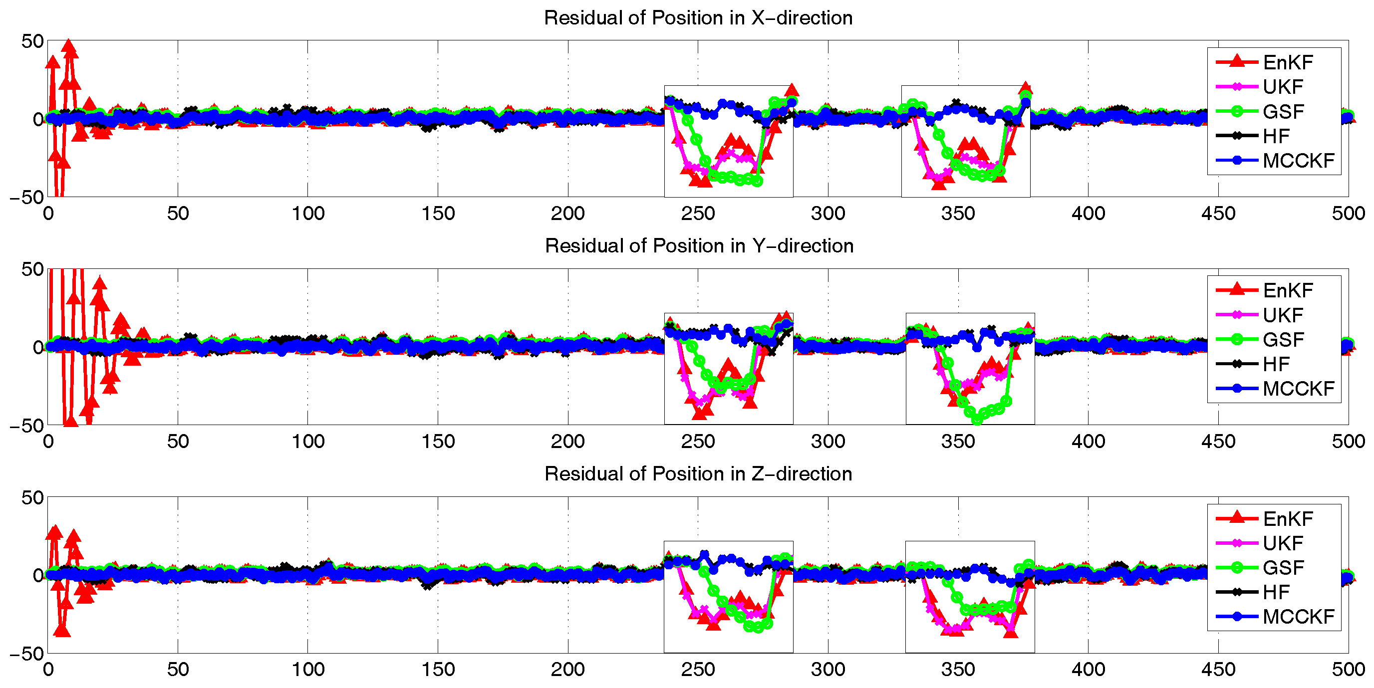
4.4. The Presence of Large Outliers

In this section, we will apply the MCCKF on $\alpha$-Jerk model in the presence of large outliers to verify the robustness of MCCKF. The simulation parameters and the initial state are the same as Section 4.1. The constant outliers are added, respectively, from 251 s to 260 s and from 351 s to 360 s. The magnitude of the outliers is 10.

To explain the advantages of MCCKF, we use the EnKF, UKF, GSF, and HF algorithms to track targets with $\alpha$-jerk models compared with MCCKF. Figure 8 demonstrates the real target trajectory and the estimated target trajectories with EnKF, GSF, UKF, HF and MCCKF in a two-dimensional plane. Figure 9 demonstrates the residual defined in Equation (79) with EnKF, UKF, GSF, HF and MCCKF.

Table 7. RMSE of every state variable in x-direction of EnKF, UKF, GSF, HF and MCCKF algorithms.

	Position (m)	Velocity (m/s)	Accelaration ($\mathbf{m}/{\mathbf{s}}^2$)	Jerk ($\mathbf{m}/{\mathbf{s}}^3$)	$\mathit{\alpha }$
EnKF	6.9390	6.4846	3.7753	0.6530	1.3750
UKF	3.3104	1.7170	0.9083	0.4238	0.9707
GSF	3.0822	1.5156	0.8306	0.4258	0.9707
HF	2.3903	1.4708	1.7734	1.3180	1.0783
MCCKF	1.4252	1.3336	0.8153	0.4245	0.9707

,

Table 8. RMSE of every state variable in y-direction of EnKF, UKF, GSF, HF and MCCKF algorithms.

	Position (m)	Velocity (m/s)	Accelaration ($\mathbf{m}/{\mathbf{s}}^2$)	Jerk ($\mathbf{m}/{\mathbf{s}}^3$)	$\mathit{\alpha }$
EnKF	3.7977	2.8730	1.7031	0.5630	5.5318
UKF	3.3085	1.6968	0.9586	0.4464	0.3219
GSF	3.5637	1.6479	0.8553	0.4259	0.3219
HF	2.2420	3.2366	1.6525	1.3194	0.8478
MCCKF	1.3119	1.2571	0.8020	0.4244	0.3219

and

Table 9. RMSE of every state variable in z-direction of EnKF, UKF, GSF, HF and MCCKF algorithms.

	Position (m)	Velocity (m/s)	Accelaration ($\mathbf{m}/{\mathbf{s}}^2$)	Jerk ($\mathbf{m}/{\mathbf{s}}^3$)	$\mathit{\alpha }$
EnKF	11.6641	9.4672	4.7836	0.8071	2.8136
UKF	3.1840	1.6303	0.9613	0.4324	0.6726
GSF	2.8279	1.3632	0.8259	0.4192	0.6726
HF	2.2469	3.2751	1.6901	1.3161	0.9380
MCCKF	1.3696	1.2799	0.8209	0.4188	0.6726

summarize the corresponding RMSE of every state variable with five algorithms in three directions.

As can be seen from Figure 8, MCCKF has a higher accuracy in most time. From Figure 9, it can be evidently seen that EnKF, UKF and GSF have divergence during the time of outliers. HF and MCCKF have a stable behavior in the whole process. Table 7, Table 8 and Table 9 show that MCCKF has a better performance than others, including HF.

4.5. The Presence of Gaussian Mixture Noises

In this section, we will apply the MCCKF on the $\alpha$-Jerk model in the presence of Gaussian mixture noises to verify the advantage of MCCKF. The simulation parameters and the initial state are also the same as Section 4.1. In the measurement process, we add the Gaussian mixture noise. The Gaussian mixture noise model is as follows:

$$\begin{array}{c}{\mathbf{V}}_k=\left(1-\upsilon \right)N\left({\mathit{\mu }}_1,{\mathit{\sigma }}_1^2\right)+\upsilon N\left({\mathit{\mu }}_2,{\mathit{\sigma }}_2^2\right),\end{array}$$

(81)

where ${\mathit{\mu }}_1=\left[\begin{array}{ccc}0& 0& 0\end{array}\right]$, ${\mathit{\mu }}_2=\left[\begin{array}{ccc}0& 0& 0\end{array}\right]$, ${\mathit{\sigma }}_1^2=\mathit{R}$, ${\mathit{\sigma }}_2^2=diag\left(\left[\begin{array}{ccc}10& 10& 10\end{array}\right]\right)$ and $\upsilon =0.01$.

The accuracy of the MCCKF is compared with the EnKF, UKF, GSF, and HF. Figure 10 demonstrates the real target trajectory and the estimated target trajectories with EnKF, UKF, GSF, HF and MCCKF. Figure 11 demonstrates the residual defined in Equation (79) with EnKF, GSF, UKF, HF and MCCKF in a two-dimensional plane. Table 8, Table 9 and

Table 10. RMSE of every state variable in the x-direction of EnKF, UKF, GSF, HF and MCCKF algorithms.

	Position (m)	Velocity (m/s)	Accelaration ($\mathbf{m}/{\mathbf{s}}^2$)	Jerk ($\mathbf{m}/{\mathbf{s}}^3$)	$\mathit{\alpha }$
EnKF	6.4009	6.4574	3.3219	0.5756	2.0893
UKF	1.3171	1.5839	1.0426	0.4578	0.9669
GSF	1.6669	1.4316	0.9840	0.4498	0.9669
HF	1.5411	1.4907	0.9834	0.4703	0.9669
MCCKF	1.3080	1.4194	0.9714	0.4497	0.9669

summarize the corresponding RMSE of every state variable with five algorithms in three directions.

Similar to the presence of large outliers, MCCKF has a higher accuracy in most time compared to other methods from Figure 10 and Figure 11. Furthermore, it can be seen that it has a better performance than others from Table 10,

Table 11. RMSE of every state variable in the y-direction of EnKF, UKF, GSF, HF and MCCKF algorithms.

	Position (m)	Velocity (m/s)	Accelaration ($\mathbf{m}/{\mathbf{s}}^2$)	Jerk ($\mathbf{m}/{\mathbf{s}}^3$)	$\mathit{\alpha }$
EnKF	5.6661	6.9973	3.8323	0.6798	1.6025
UKF	1.2481	1.4203	0.9216	0.4233	1. 5972
GSF	1.6537	1.2715	0.8655	0.412	1. 5972
HF	1.2348	1.2715	0.8655	0.4122	1. 5972
MCCKF	1.0214	1.2607	0.8226	0.4117	1.5972

and

Table 12. RMSE of every state variable in the z-direction of EnKF, UKF, GS, HF and MCCKF algorithms.

	Position (m)	Velocity (m/s)	Accelaration ($\mathbf{m}/{\mathbf{s}}^2$)	Jerk ($\mathbf{m}/{\mathbf{s}}^3$)	$\mathit{\alpha }$
EnKF	2.4590	2.6990	1.5505	0.5314	3.0559
UKF	1.2806	1.5766	1.0119	0.4717	0.4726
GSF	1.5664	1.3625	0.9533	0.4678	0.4726
HF	1.2877	1.3625	0.9529	0.4678	0.4726
MCCKF	1.2548	1.3602	0.9134	0.4678	0.4726

.

5. Conclusions

$\alpha$-jerk model, a modified jerk model, can estimate the parameter $\alpha$ in real time during the process of target tracking. In the process of tracking targets, the measurement noise is a research focus. Large outliers and Gaussian mixture noises are the most popular non-Gaussian noises in the measurement process. Maximum Correntropy Criterion Kalman Filter is deduced with the weighted least square algorithm, which is proved to be rational based on the correntropy theory. Its robustness in the state estimation is analyzed with influence function for the first time. It proves that the filter algorithm can overcome the influence of non-Gaussian noises. Furthermore, a novel kernel size selection is proposed, which can improve the robustness of the filter algorithm. Simulated experimental results demonstrate that it provides effective performance to control the non-Gaussian noises of $\alpha$-jerk model.

References

1. Li, X.R.; Jilkov, V.P. Survey of maneuvering target tracking. Part I. Dynamic models. IEEE Trans. Aerosp. Electron. Syst. 2004, 39, 1333–1364. [Google Scholar]
2. Yang, X.; Xing, K.; Feng, X. Maneuvering target tracking in dense clutter based on particle filtering. Chin. J. Aeronaut. 2011, 24, 171–180. [Google Scholar] [CrossRef]
3. Singer, R.A. Estimating optimal tracking filter performance for manned maneuvering targets. IEEE Trans. Aerosp. Electron. Syst. 1970, AES-6, 473–483. [Google Scholar] [CrossRef]
4. Bar-Shalom, Y.; Birmiwal, K. Variable dimension filter for maneuvering target tracking. IEEE Trans. Aerosp. Electron. Syst. 1982, AES-18, 621–629. [Google Scholar] [CrossRef]
5. Kumar, K.S.P.; Zhou, H.; Kumar, K.S.P.; Zhou, H. A “current” statistical model and adaptive algorithm for estimating maneuvering targets. J. Guidance Control Dyn. 1984, 7, 596–602. [Google Scholar] [CrossRef]
6. Mehrotra, K.; Mahapatra, P.R. A jerk model for tracking highly maneuvering targets. IEEE Trans. Aerosp. Electron. Syst. 1997, 33, 1094–1105. [Google Scholar] [CrossRef]
7. Luo, X.B. A α-jerk model for tracking maneuvering targets. Signal Process. 2007, 4, 481–484. [Google Scholar]
8. Li, X.R.; Jilkov, V.P. A survey of maneuvering target tracking: Approximation techniques for nonlinear filtering. Proc. SPIE 2004, 5428. [Google Scholar] [CrossRef]
9. Roth, M.; Hendeby, G.; Fritsche, C.; Gustafsson, F. The ensemble kalman filter: A signal processing perspective. Eurasip J. Adv. Signal Process. 2017, 2017, 56. [Google Scholar] [CrossRef]
10. Ammann, N.; Andert, F. Visual navigation for autonomous, precise and safe landing on celestial bodies using unscented kalman filtering. In Proceedings of the 2017 IEEE Aerospace Conference, Big Sky, MT, USA, 4–11 March 2017. [Google Scholar]
11. Zhang, C.; Hwang, I. Gaussian sum-based maneuvering target tracking using unmanned aerial vehicle. In Proceedings of the AIAA Guidance, Navigation, and Control Conference, Grapevine, TX, USA, 9–13 January 2017; pp. 1–12. [Google Scholar]
12. Julier, S.J.; Uhlmann, J.K.; Durrant-Whyte, H.F. A new approach for filtering nonlinear systems. In Proceedings of the American Control Conference, Seattle, WA, USA, 21–23 June 1995; Volume 3, pp. 1628–1632. [Google Scholar]
13. Uhlmann, J.K.; Julier, S.J. A new extension of the kalman filter to nonlinear systems. Proc. SPIE 1997, 3068, 182–193. [Google Scholar]
14. Maybeck, P.S. Stochastic Models, Estimation and Control Volume 3; Academic Press: New York, NY, USA, 1979. [Google Scholar]
15. Stein, D.W.J. Detection of random signals in gaussian mixture noise. In Proceedings of the 1994 28th Asilomar Conference on Signals, Systems and Computers, Pacific Grove, CA, USA, 31 October–2 November 1994; Volume 2, pp. 791–795. [Google Scholar]
16. Wu, W.R. Target racking with glint noise. IEEE Trans. Aerosp. Electron. Syst. 1993, 29, 174–185. [Google Scholar]
17. Plataniotis, K.N.; Androutsos, D.; Venetsanopoulos, A.N. Nonlinear filtering of non-gaussian noise. J. Intell. Robot. Syst. 1997, 19, 207–231. [Google Scholar] [CrossRef]
18. Sorenson, H.W.; Alspach, D.L. Recursive bayesian estimation using gaussian sums. Automatica 1971, 7, 465–479. [Google Scholar] [CrossRef]
19. Harvey, A.; Luati, A. Filtering with heavy tails. J. Am. Stat. Assoc. 2014, 109, 1112–1122. [Google Scholar] [CrossRef]
20. Izanloo, R.; Fakoorian, S.A.; Yazdi, H.S.; Dan, S. Kalman filtering based on the maximum correntropy criterion in the presence of non-gaussian noise. In Proceedings of the Information Science and Systems, Princeton, NJ, USA, 16–18 March 2016; pp. 500–505. [Google Scholar]
21. Wan, E.A.; van der Merwe, R. The unscented Kalman filter for nonlinear estimation. In Proceedings of the IEEE 2000 Adaptive Systems for Signal Processing, Communications, and Control Symposium, Lake Louise, AB, Canada, 4 October 2000; pp. 153–158. [Google Scholar]
22. Curn, J.; Marinescu, D.; Lacey, G.; Cahill, V. Estimation with non-white gaussian observation noise using a generalised ensemble kalman filter. In Proceedings of the IEEE International Symposium on Robotic and Sensors Environments, Magdeburg, Germany, 16–18 November 2012; pp. 85–90. [Google Scholar]
23. Kotecha, J.H.; Djuric, P.M. Gaussian sum particle filtering. IEEE Trans. Signal Process. 2003, 51, 2602–2612. [Google Scholar] [CrossRef]
24. Liu, Y.; Dong, K.; Wang, H.; Liu, J.; He, Y.; Pan, L. Adaptive gaussian sum squared-root cubature kalman filter with split-merge scheme for state estimation. Chin. J. Aeronaut. 2014, 27, 1242–1250. [Google Scholar] [CrossRef]
25. Yin, J.; Zhang, J.; Zhuang, Z. Gaussian sum phd filtering algorithm for nonlinear non-gaussian models. Chin. J. Aeronaut. 2008, 21, 341–351. [Google Scholar]
26. Rousseeuw, P.J.; Leroy, A.M. Robust Regression and Outlier Detection. J. R. Stat. Soc. 1989, 152, 133–134. [Google Scholar]
27. Wang, R.; Xiong, Z.; Liu, J.Y.; Li, R.; Peng, H. SINS/GPS/CNS information fusion system based on improved huber filter with classified adaptive factors for high-speed UAVs. In Proceedings of the 2012 IEEE/ION Position Location and Navigation Symposium (PLANS), Myrtle Beach, SC, USA, 23–26 April 2012; pp. 441–446. [Google Scholar]
28. Huang, J.; Yan, B.; Hu, S. Centralized fusion of unscented kalman filter based on huber robust method for nonlinear moving target tracking. Math. Probl. Eng. 2015, 2015, 291913. [Google Scholar] [CrossRef]
29. Chang, L.; Li, K.; Hu, B. Huber’s m-estimation-based process uncertainty robust filter for integrated ins/gps. IEEE Sens. J. 2015, 15, 3367–3374. [Google Scholar] [CrossRef]
30. Chien-Hao, T.; Lin, S.F.; Dah-Jing, J. Robust huber-based cubature kalman filter for gps navigation processing. J. Navigat. 2016, 70, 527–546. [Google Scholar]
31. Chang, G. Robust kalman filtering based on mahalanobis distance as outlier judging criterion. J. Geodesy 2014, 88, 391–401. [Google Scholar] [CrossRef]
32. Rodger, J.A. Toward reducing failure risk in an integrated vehicle health maintenance system: A fuzzy multi-sensor data fusion kalman filter approach for ivhms. Expert Syst. Appl. 2012, 39, 9821–9836. [Google Scholar] [CrossRef]
33. Chen, B.; Liu, X.; Zhao, H.; Principe, J.C. Maximum correntropy kalman filter. Automatica 2017, 76, 70–77. [Google Scholar] [CrossRef]
34. Liu, X.; Qu, H.; Zhao, J.; Yue, P.; Wang, M. Maximum correntropy unscented kalman filter for spacecraft relative state estimation. Sensors 2016, 16, 1530. [Google Scholar] [CrossRef] [PubMed]
35. Liu, X.; Chen, B.; Xu, B.; Wu, Z.; Honeine, P. Maximum correntropy unscented filter. Int. J. Syst. Sci. 2017, 48, 1607–1615. [Google Scholar] [CrossRef]
36. Xi, L.; Hua, Q.; Zhao, J.; Chen, B. Extended Kalman filter under maximum correntropy criterion. In Proceedings of the International Joint Conference on Neural Networks, Vancouver, BC, Canada, 24–29 July 2016; pp. 1733–1737. [Google Scholar]
37. Wang, J.J.-Y.; Wang, Y.; Jing, B.-Y.; Gao, X. Regularized maximum correntropy machine. Neurocomputing 2015, 160, 85–92. [Google Scholar] [CrossRef]
38. Li, X.R.; Jilkov, V.P. Survey of maneuvering target tracking. Part V. multiple-model methods. IEEE Trans. Aerosp. Electron. Syst. 2005, 41, 1255–1321. [Google Scholar]
39. Lewis, F.L. Applied optimal control. IEEE Trans. Autom. Control 2003, 17, 186–188. [Google Scholar]
40. Jiang, C.; Zhang, S.B.; Zhang, Q.Z. A new adaptive h-infinity filtering algorithm for the GPS/INS integrated navigation. Sensors 2016, 16, 21–27. [Google Scholar] [CrossRef] [PubMed]
41. Príncipe, J.C. Information Theoretic Learning: Renyi’s Entropy and Kernel Perspectives; Springer Publishing Company, Incorporated: Berlin, Germany, 2010. [Google Scholar]
42. Chen, B.; Xing, L.; Liang, J.; Zheng, N.; Príncipe, J.C. Steady-state mean-square error analysis for adaptive filtering under the maximum correntropy criterion. IEEE Signal Process. Lett. 2014, 21, 880–884. [Google Scholar]
43. Chen, B.; Wang, J.; Zhao, H.; Zheng, N.; Príncipe, J.C. Convergence of a fixed-point algorithm under maximum correntropy criterion. IEEE Signal Process. Lett. 2015, 22, 1723–1727. [Google Scholar] [CrossRef]
44. Chen, B.; Príncipe, J.C. Maximum correntropy estimation is a smoothed map estimation. IEEE Signal Process. Lett. 2012, 19, 491–494. [Google Scholar] [CrossRef]
45. Liu, W.; Pokharel, P.P.; Príncipe, J.C. Correntropy: Properties and applications in non-gaussian signal processing. IEEE Trans. Signal Process. 2007, 55, 5286–5298. [Google Scholar] [CrossRef]
46. He, R.; Hu, B.; Yuan, X.; Wang, L. Robust Recognition via Information Theoretic Learning; Springer International Publishing: Berlin, Germany, 2014. [Google Scholar]
47. Huber, P.J. Robust estimation of a location parameter. Ann. Math. Stat. 1964, 35, 73–101. [Google Scholar] [CrossRef]
48. Chang, G.; Liu, M. M-estimator-based robust kalman filter for systems with process modeling errors and rank deficient measurement models. Nonlinear Dyn. 2015, 80, 1431–1449. [Google Scholar] [CrossRef]
49. Chang, G.; Xu, T.; Wang, Q. M-estimator for the 3d symmetric helmert coordinate transformation. J. Geodesy 2017, 2017, 1–12. [Google Scholar] [CrossRef]
50. He, Y.; Wang, F.; Yang, J.; Rong, H.; Chen, B. Kernel adaptive filtering under generalized maximum correntropy criterion. In Proceedings of the International Joint Conference on Neural Networks, Vancouver, BC, Canada, 24–29 July 2016; pp. 1738–1745. [Google Scholar]
51. Wang, Y.; Zheng, W.; Sun, S.; Li, L. Robust information filter based on maximum correntropy criterion. J. Guidance Control Dyn. 2016, 39, 1–6. [Google Scholar] [CrossRef]
52. Huber, P.J. The 1972 wald lecture robust statistics: A review. Ann. Math. Stat. 1972, 43, 1041–1067. [Google Scholar] [CrossRef]
53. Taylor, A.E. L’hospital’s rule. Am. Math. Mon. 1952, 59, 20–24. [Google Scholar] [CrossRef]
54. He, R.; Zheng, W.S.; Hu, B.G. Maximum correntropy criterion for robust face recognition. IEEE Trans. Pattern Anal. Mach. Intell. 2011, 33, 1561–1576. [Google Scholar] [PubMed]
55. Liu, W.; Príncipe, J.C.; Haykin, S.S. Kernel Adaptive Filtering: A Comprehensive Introduction; John Wiley & Sons: Hoboken, NJ, USA, 2010. [Google Scholar]
56. Cinar, G.T.; Príncipe, J.C. Hidden state estimation using the correntropy filter with fixed point update and adaptive kernel size. In Proceedings of the 2012 International Joint Conference on Neural Networks (IJCNN), Brisbane, Australia, 10–15 June 2012. [Google Scholar]
Figure 1. Correntropy when λ = 1 .
Entropy 19 00648 g001
Figure 2. ψ with different estimation errors in different weighting functions.
Entropy 19 00648 g002
Figure 3. ψ with different kernel size selection methods (where λ 0 is the novel kernel size selection method).
Entropy 19 00648 g003
Figure 4. Target trajectories of two kernel size adaptive methods on α -jerk model where λ 0 is the novel kernel size adaptive method.
Entropy 19 00648 g004
Figure 5. Residual of estimated position with two kernel size adaptive methods where λ 0 is the novel kernel size adaptive method.
Entropy 19 00648 g005
Figure 6. Target trajectories of different filter algorithms on the α -jerk model in the presence of Gaussian noises.
Entropy 19 00648 g006
Figure 7. Residual of estimated position with different filter algorithms in the presence of Gaussian noises.
Entropy 19 00648 g007
Figure 8. Target trajectories of different filter algorithms on α -jerk model in the presence of large outliers.
Entropy 19 00648 g008
Figure 9. Residual of estimated position with different filter algorithms in the presence of large outliers.
Entropy 19 00648 g009
Figure 10. Target trajectories of different filter algorithms on the α -jerk model in the presence of Gaussian mixture noises.
Entropy 19 00648 g010
Figure 11. Residual of estimated position with different filter algorithms in the presence of Gaussian mixture noises.
Entropy 19 00648 g011