
Nonlinear Wave Equations Related to Nonextensive Thermostatistics


1
CeBio y Secretaría de Investigación, Universidad Nacional del Noroeste de la Província de Buenos Aires, UNNOBA-Conicet, Roque Saenz Peña 456, 6000 Junin, Argentina
2
Instituto de Matemática e Estatística, Universidade do Estado do Rio de Janeiro, Rua São Francisco Xavier, 524, 20550-900 Rio de Janeiro, Brazil
*
Author to whom correspondence should be addressed.
Entropy 2017, 19(2), 60; https://doi.org/10.3390/e19020060
Submission received: 25 December 2016
/
Revised: 31 January 2017
/
Accepted: 4 February 2017
/
Published: 7 February 2017
(This article belongs to the Special Issue Entropic Aspects of Nonlinear Partial Differential Equations: Classical and Quantum Mechanical Perspectives)
Abstract
:We advance two nonlinear wave equations related to the nonextensive thermostatistical formalism based upon the power-law nonadditive entropies. Our present contribution is in line with recent developments, where nonlinear extensions inspired on the q-thermostatistical formalism have been proposed for the Schroedinger, Klein–Gordon, and Dirac wave equations. These previously introduced equations share the interesting feature of admitting q-plane wave solutions. In contrast with these recent developments, one of the nonlinear wave equations that we propose exhibits real q-Gaussian solutions, and the other one admits exponential plane wave solutions modulated by a q-Gaussian. These q-Gaussians are q-exponentials whose arguments are quadratic functions of the space and time variables. The q-Gaussians are at the heart of nonextensive thermostatistics. The wave equations that we analyze in this work illustrate new possible dynamical scenarios leading to time-dependent q-Gaussians. One of the nonlinear wave equations considered here is a wave equation endowed with a nonlinear potential term, and can be regarded as a nonlinear Klein–Gordon equation. The other equation we study is a nonlinear Schroedinger-like equation.
1. Introduction
In the present paper, we introduce and investigate some features of two nonlinear wave equations related to the nonextensive thermostatistical formalism [1,2,3]. This work is motivated by a recent line of enquiry concerning nonlinear extensions of the Schroedinger, Dirac, and Klein–Gordon equations also linked to this formalism [4,5,6,7,8,9,10,11,12,13]. These nonlinear equations, in turn, exhibit close formal similarities with a family of nonlinear Fokker–Planck equations that govern the evolution of a variegated class of systems and processes in physics, biology and other fields, and have been the focus of intense research efforts in recent years [14,15,16,17,18,19,20,21].
The nonlinear Schroedinger, Dirac, and Klein–Gordon equations previously explored in [4,5,6,7,8,9,10,11,12,13] exhibit the interesting feature of having soliton-like analytical solutions that behave as free particles, in the sense that they satisfy the Einstein–Planck–de Broglie relations [4]. The wave function corresponding to these solutions depends on the spatial coordinate x and on time t through the quantity . This means that the evolution of the wave function is given by a uniform translation at a constant speed v without change in shape. These exact solutions have the form of q-plane waves, which can be regarded as complex valued analogues of the q-exponential distributions appearing at the core of the nonextensive thermostatistics [2].
The nonextensive thermostatistical formalism and its applications constitutes nowadays an active research field involving scientists working in diverse fields. This formalism was first introduced as a generalization of the maximum entropy approach to Gibbs statistical mechanics [3]. It is based on the family of power-law entropic functionals, which was in turn inspired in the study of multifractals [2,3]. Some of the earliest (and, by now, most developed) applications of the formalism were to non-equilibrium (or meta-equilibrium) states of systems with long-range interactions (see, for instance, [1]) and to dynamical systems exhibiting weak chaos (see [22] and references therein). However, the mathematical apparatus associated with the nonextensive thermostatistics turned out to be useful for the study of a surprising variety of problems in physics, biology, and other fields. In the case of physics, applications have been developed both within the classical and the quantum mechanical domains [2]. These applications involve the q-exponential and q-Gaussian functions, that arise naturally within this theoretical framework. These functions reduce to the standard exponential and Gaussian ones in the limit. Just to list a few recent examples of applications of the nonextensive thermostatistical formalism, we can mention applications to self-gravitating systems [23], to the dynamics of vortices in type II superconductors [19], and to complex networks [24]. The remarkably diverse scenarios within which q-exponentials and q-Gaussians appear to be relevant suggests that the dynamical mechanisms giving rise to these distributions are not unique. That is, it seems likely that there is more than one (and probably several) possible dynamical processes leading to q-exponentials and to q-Gaussians.
The nonlinear wave equations that we are going to consider here, in contrast to the aforementioned previously studied nonlinear Schroedinger, Klein–Gordon, and Dirac equations, have either real q-Gaussian solutions or exponential plane wave solutions modulated by a q-Gaussian, instead of complex q-plane wave ones. The q-Gaussians are q-exponentials with an argument that is a quadratic function of the relevant spatial or phase-space variables. As already mentioned, the q-Gaussian functions play a central role within the nonextensive thermostatistical formalism and its multiple applications, and are observed in a wide variety of natural phenomena [1,2,22,25,26]. Consequently, it is of the foremost importance to identify and explore all the possible dynamical mechanisms that may generate q-Gaussians. Some non-conservative dynamical processes admitting exact analytical (real) q-Gaussian solutions have been investigated by researchers in detail in recent years. Prominent among them are the processes described by nonlinear power-law Fokker–Planck equations (see, for instance, [14,15,16,17,18,19,20,21] and references therein). On the contrary, continuous (as opposed to discrete) conservative dynamical systems exhibiting exact, time-dependent, real, q-Gaussian solutions remain largely unexplored. One of the purposes of the present contribution is to advance a nonlinear wave equation having precisely these properties. We are also going to discuss a Schroedinger nonlinear equation exhibiting q-Gaussian wave packet solutions.
The paper is organized as follows. In Section 2, we briefly review the main partial differential evolution equations related to the nonextensive thermostatistical formalism. In Section 3, we introduce and explore the main properties of a nonlinear wave equation having q-Gaussian solutions. In Section 4, we consider a Schroedinger-like equation exhibiting q-Gaussian wave packet solutions. Finally, some conclusions are drawn in Section 5.
2. Nonlinear Partial Differential Evolution Equations Associated with the Nonextensive Thermostatistical Formalism
The nonextensive thermostatistical formalism is based on the nonadditive, power-law entropic functional [2] given by
where q is a real parameter and is a probability density. In the limit , the entropy reduces to the standard Boltzmann–Gibbs logarithmic entropy, .
The so-called q-exponential function, arising when considering constrained optimization problems based on the entropic measure , plays a central role within the nonextensive thermostatistical formalism [1,2,24]. This function is defined as
An alternative notation for q-exponentials, which we are going to follow in this work, is given by .
Of particular interest are the q-Gaussian distributions, which are proportional to q-exponentials whose argument is quadratic in the relevant space or phase-space variables. For instance, one dimensional q-Gaussians are proportional to , where λ is a real positive parameter determining the width of the q-Gaussian. These distributions are relevant for the study of a wide family of systems and processes in physics, biology and other areas [1,2]. They arise naturally as solutions, both of the stationary and of the time-dependent kind, of some partial differential equations of mathematical physics. The first partial differential equation for which a connection with the entropy was established was the nonlinear Fokker–Planck (NLFP) equation with a power-law nonlinearity [15]. This NLFP equation has (in one spatial dimension) the form
where is a time-dependent density, D is a diffusion constant, and is a potential function. For quadratic potentials, the power-law NLFP equation admits exact time-dependent solutions, of the q-Gaussian form. The connection between the power-law NLFP equation and the entropy (1) has originated intense research activity. Several extensions and applications of the NLFP– connection have been explored over the years [14,15,16,17,18,19,20,21]. It has to be stressed that the NLFP equation describes a non-conservative dynamics.
In 2011, Nobre, Rego-Monteiro and Tsallis (NRT) advanced a nonlinear version of the Schroedinger equation [4] that has a formal similarity with the power-law NLFP equation
where is a time-dependent wave function, m is a constant with dimensions of mass, ℏ is Planck`s constant, is a constant that guarantees that all the terms in the equation have the same dimensions, and . In the limit , the standard, linear Schroedinger equation is recovered.
In spite of the already mentioned formal similarities between the NLFP and the NRT equations, the properties of these two equations are very different. The NLFP equation is a real equation with real-valued solutions, while the NRT equation clearly involves complex numbers and, in general, has complex-valued solutions. The NLFP equation satisfies an H-theorem, while the NRT equation admits particular traveling solutions exhibiting a soliton-like behavior. The most important solutions of the NRT equation, which highlight its close connection with the nonextensive thermostatistical formalism, are the q-plane waves. These solutions are written in terms of q-exponentials with non-real arguments,
where the constants w and k satisfy , akin to the relation between the energy and momentum of a non-relativistic particle of mass m. The q-plane wave solutions (5) are expressed in terms of the q-exponential function, with a pure imaginary argument . This is defined as the principal value of
with real and imaginary parts respectively given by
with .
Our aim in the present effort is to introduce two wave equations related to the nonextensive thermostatistics that, in contrast with the NRT equation, admit exact analytical time-dependent solutions involving q-Gaussian functions. This is a property that the wave equations advanced here share with the NLFP equation. However, the proposed wave equations differ from the NLFP in one essential aspect: they describe a conservative dynamics.
3. Nonlinear Wave Equation with q-Gaussian Solutions
We are going to consider a family of nonlinear wave equations of the form
where v, η, q, and are real constant parameters. The quantity v is a constant with dimensions of velocity, η is a constant with dimensions of inverse squared length, q is a nondimensional constant, and the constant guaranties that each term in (8) has the same dimensionality. It is convenient to work with the dimensionless quantity , satisfying the evolution equation
We propose, as a solution of the nonlinear wave Equation (9), the space-time dependent, real, q-Gaussian ansatz
where is a dimensionless real parameter, is a real parameter with dimensions of inverse time and is a real parameter with dimensions of inverse length. It is convenient to define the dimensionless variable . The function is equal to when and vanishes when . The points at which are called the cut-off points. For , there are no cut-off points, and ψ is everywhere non-vanishing. In the limit , the q-Gaussian adopts a standard exponential Gaussian form. We regard the nonlinear wave Equation (9) as describing a classical field. Consequently, the solutions are not required to be normalized.
At those points where , one has
Replacing in the last two of the above equations, one obtains
Note that for , the functions , , , , and , all go to zero continuously at the cut-off points. Since the q-Gaussian ansatz (10) is always real and nonnegative, one has and .
It follows from (12) that the time-dependent, q-Gaussian ansatz (10) constitutes an exact analytical solution of the nonlinear wave Equation (9), provided that the relation
is verified. The shape of this solution is exhibitted in Figure 1 for different values of q.
The solution (10) exhibits a soliton-like behavior, in the sense of being a solution that propagates at a constant velocity without changing form. The propagation velocity is given by . In the case , the nonlinear wave Equation (9) is reduced to the standard linear wave equation, with wave velocity v. The two velocities u and v are related through
The time-dependent wave packet solution (10) is centered at
The center of the wave packet, of course, moves at the uniform velocity . The width of the wave packet is determined by the modulus of the parameter , so that increasing values of correspond to more localized wave packets. It transpires from Equation (14) that the velocity u of the q-Gaussian wave packets depends on their width. For , the propagation velocity u of the q-Gaussian solutions is greater than the wave velocity v of the linear wave equation, and u decreases with the degree of localization of the wave packets. On the contrary, when , the q-Gaussian wave packets move at velocities smaller than v, and wave packets of increasing localization move at greater velocities. In both cases, as the wave packets become more localized, their propagation velocity tends to the wave velocity v of the linear wave equation. When , one recovers the linear wave equation where the propagation velocity is, of course, independent of the width of the wave packets.
The q-Gaussian wave packet solution can be written explicitly in terms of the wave packet’s center as . As already mentioned, for , this wave packet has a finite amplitude only on a finite range of x-values comprised within the cut-off points, , where is the width of the wave packet. Let us call this localized q-Gaussian a “q-Gaussian pulse”. It is evident that is also a q-Gaussian pulse solution of the nonlinear wave Equation (9). Using the fact that , , and , all go to zero at the cut-off points, it is possible to match an infinite sequence of q-Gaussian pulses of alternating signs at their turning points, and construct a new solution consisting of a wave-like infinite train of pulses, defined in a piece-wise way by
This train of pulses moves at the constant uniform velocity , and exhibits a traveling wave-like pattern, consecutive pulses being of alternating signs, all of them having the same width Δ, and the nth pulse centered at . However, the pulses have a q-Gaussian shape, instead of half-sinusoidal one.
Introducing now the potential function
it is possible to recast the wave Equation (9) under the guise
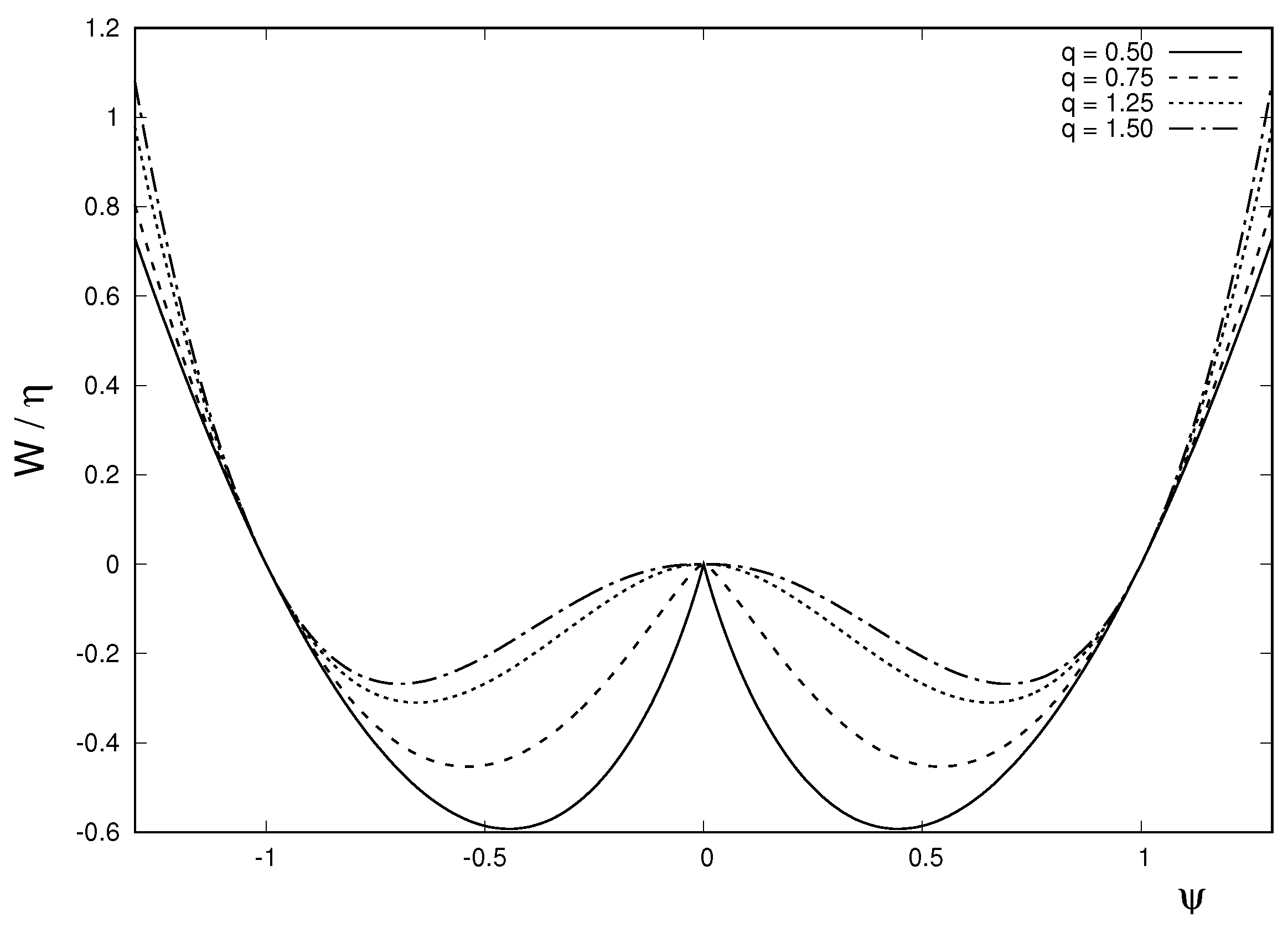
where . The wave Equation (18) has the form of a nonlinear Klein–Gordon equation. The shape of the potential is shown in Figure 2 for different q-values.
If we regard the nonlinear wave Equation (9) as governing the evolution of a real field , then the wave equation can be derived from the Lagrangian density
Indeed, the Euler–Lagrange equation,
where and , corresponds to the wave Equation (9). When regarded as describing a real field, the nonlinear wave Equation (9) admits a classical mechanical interpretation. It can be construed as governing the time evolution of a vibrating string, subjected to the effect of a lateral force field described by the potential (17). The vibration of the string is assumed to be constrained to a plane and corresponds to the lateral displacement of the string.
The appropriate Lagrangean density for a complex field , governed by the wave Equation (9), is
where the potential W, explicitly written in terms of the field ψ and its complex conjugate , is
The Euler–Lagrange equations associated with the Lagrangean (21) are
The first of the above equations is precisely the wave Equation (9), while the second one is the complex conjugate of (9).
Finally, let us consider the limit of the evolution Equation (9). In this limit, this equation becomes
We see that the nonlinearity in the wave Equation (9), which is proportional to the difference between two powers of , in the limit gives rise to a logarithmic nonlinearity. We are going to find again a logarithmic nonlinearity in Section 4, when discussing the limit of another nonlinear wave equation. Logarithmic nonlinearities have applications in quantum physics (see the comment in Section 4, after Equation (33)). In the limit of the nonlinear wave Equation (9), the space-time dependent q-Gaussian solution (10) reduces to the time-dependent Gaussian solution,
This solution is a pulse exhibiting a Gaussian profile, that propagates with a constant velocity and without changing shape.
4. A Nonlinear Schroedinger Equation with q-Gaussian-Modulated Wave Packet Solutions
We shall now discuss a nonlinear Schroedinger equation admitting wave packet solutions given by an exponential plane wave modulated by a q-Gaussian. Let us consider the wave equation,
where m, γ, q, and are real constant parameters, ℏ is Planck’s constant and i is the imaginary unit. The quantity m is a constant with dimensions of mass, γ is a constant with dimensions of energy, q is a dimensionless constant, and the constant guaranties that each term in (26) has the same dimensionality. As in the case of the wave equation considered in the previous section, it is convenient to work with the dimensionless quantity , which now satisfies the evolution equation
Now we propose the wave packet ansatz,
with real constant parameters k, ω, , and . The parameters k and have dimensions of inverse length, ω and have dimensions of inverse time, and is dimensionless. It will be convenient to rewrite the above ansatz as
with and . It follows from these definitions that, when ,
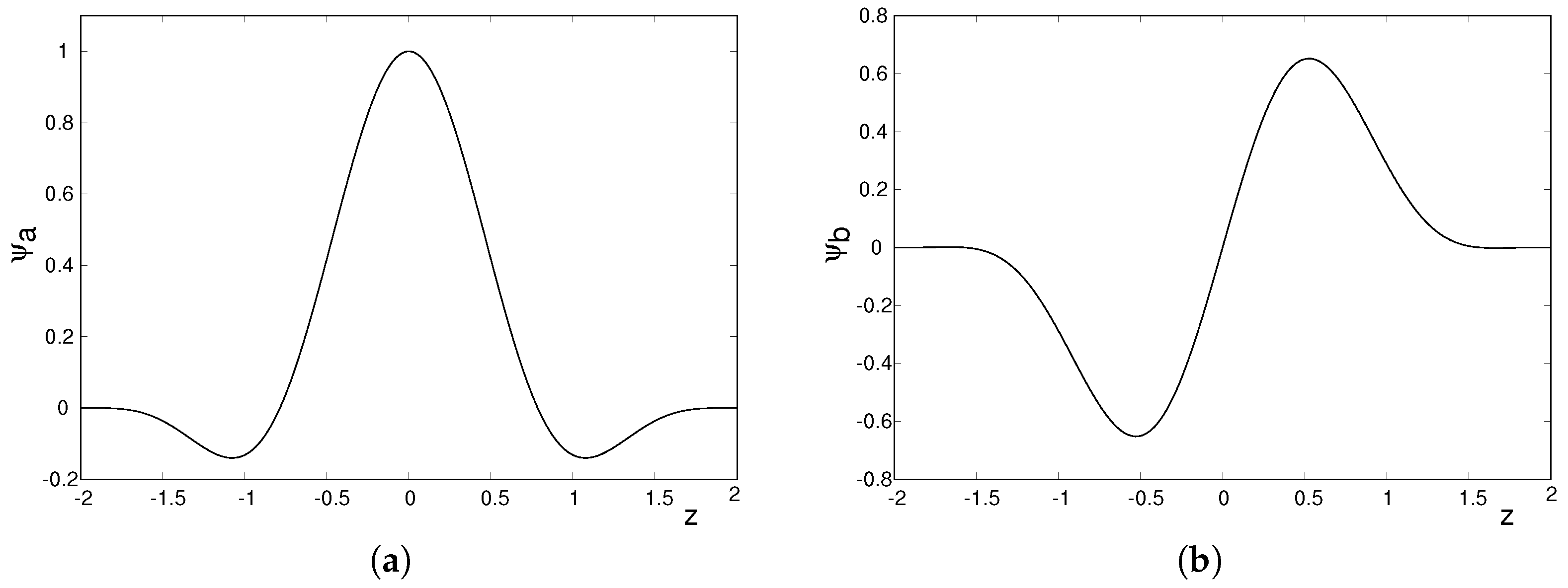
For , the wave function has two cut-off points corresponding to the points where . We then have when . For , the quantities and (besides itself) tend to zero, as we approach the cut-off points from within the region where is non-vanishing. For , there are no cut-off points. In what follows, we are going to consider only values of q larger than . As an illustrative example, the shapes of the real and imaginary parts of the wave function are given in Figure 3 for .
It follows from the above considerations that the ansatz (28) constitutes a solution of the nonlinear Schroedinger Equation (27), provided that the parameters appearing in satisfy the relations
The solution of the nonlinear Schroedinger Equation (27) can be construed as an exponential plane wave, modulated by a q-Gaussian. The parameters ω and k, appearing in this plane wave, satisfy the usual free particle relation, corresponding to the plane wave solutions of the standard linear Schroedinger equation associated with a free particle.
The Schroedinger Equation (27) can be derived from the lagrangean density,
It is interesting to consider the limit of the nonlinear Schroedinger Equation (27). In this limit, we get a Schroedinger equation with a logarithmic nonlinearity,
Schroedinger equations with logarithmic nonlinearities have been studied in the research literature [27,28,29,30]. They have been proposed to model various quantum mechanical phenomena, such as, for instance, the behavior of a quantum particle whose position is continuously being measured [28].
The nonlinear Schroedinger Equation (27) is compatible with a probabilistic interpretation of . Indeed, it can be verified that it complies with the standard conservation of probability law,
where the probability density current is,
The Schroedinger Equation (27) also admits an energy-like conserved quantity,
It can be verified after some algebra that .
It is of interest to consider briefly the nonlinear Schroedinger Equation (27) in connection with the de Broglie–Bohm model of quantum mechanics. Using the representation
the dynamics corresponding to the wave Equation (27) is equivalent to the following evolution equations for and ,
and
According to the Bohmian model of quantum mechanics, a quantum particle has a definite position and velocity at a given time, but we cannot have direct knowledge of these variables (see, for instance, [8] and references therein). The velocity of the Bohmian particle is given by . The probability density corresponding to the possible locations of the Bohmian particle is described by . Consequently, Equation (39) is the continuity equation of the probability density of the Bohmian particle. Both Equations (38) and (39) jointly govern the evolution of the probability density and of the field . This last function, in turn, determines the velocity field of the Bohmian particle.
In the case of the q-Gaussian wave packet , given by (28), the quantities and have the form,
It follows that the q-Gaussian wave packet implies a uniform Bohmian velocity field,
which coincides with the Bohmian velocity field associated with a plane wave solution of the standard, linear Schroedinger equation. Therefore, the wave packet (28) has the same velocity field as the standard plane wave, but its density differs from the (uniform) one associated with the plane wave. This anomalous density, however, evolves according to the continuity equation associated with the plane wave velocity field. This state of affairs reminds us of the intriguing extension of quantum physics proposed by Valentini, where densities differing from the ones stipulated by the strictures of standard quantum mechanics are considered (see [31,32,33] and references therein).
Up to now, we have not explicitly considered the normalization of the wave packet (28). When considering physical applications requiring a normalized wave function, one has to use the dimensional solution (as opposed to the dimensionless one ; see the comment after Equation (26)). A similar situation occurs in the case of the NRT equation [4] (see Equation (4)). The dimensional solution is,
This wave packet is normalizable for .
It is instructive to compare the main features of the nonlinear wave Equation (27) with those of the NRT Equation (4). These two nonlinear Schroedinger equations have particular analytical solutions that are related to the nonextensive thermostatistical formalism. In both cases, the squared modulus of these special solutions are q-Gaussian distributions that move with a constant velocity and without changing shape. q-Gaussian distributions play a central role in nonextensive thermostatistics and its multiple applications. They arise naturally when optimizing the power-law, entropic measure , under simple constraints. Even though the profiles of the squared modulus of the special solutions of Equation (27) and of the NRT equation are both q-Gaussians, the detailed structures of these solutions are very different. The solutions of Equation (27) are given by the product of a q-Gaussian and a standard complex exponential plane wave, while the solutions of the NRT equation are complex q-plane waves. This might suggest that the NRT is more deeply connected with the nonextensive thermostatistics than the Schroedinger Equation (27). On the other hand, the NRT equation represents a more radical departure form the standard, linear Schroedinger equation than the wave Equation (27). The NRT equation has its nonlinearity within the Laplacian term, while the nonlinearity of Equation (27) is in a potential-like term, which can be regarded as arising from an effective potential that depends on the wave function itself. Nonlinearities of this kind have been used in the literature to model different quantum effects (see, for instance, the logarithmic nonlinearity considered in [27,28]). The special solutions of the NRT equation behave in a soliton-like way, in the sense that they move with uniform velocity and without changing shape. The special solutions of Equation (27) do not, strictly speaking, exhibit this property (although their squared modulus does) because the two factors appearing in (29) move at different velocities. Equation (27) preserves the normalization of the time-dependent wave function, while the NRT equation does not, in general, preserve it (it admits, however, particular solutions whose normalization is preserved). Equation (27) can be derived from a Lagrangean involving only the wave function ψ and its complex conjugate. The NRT can be brought into a Lagrangean formulation, but only paying the price of introducing a new complex field [5]. Some of these differences (in particular, those related to the preservation of normalization) arise from the fact that the nonlinear Schroedinger Equation (27) can be obtained from a Lagrangean that is invariant under the transformation , while the NRT equation cannot. Last, but certainly not least, the q-plane wave solutions of the NRT equation behave like free particles, in the sense of being compatible with the Einstein–de Broglie relations [4]. The special solutions of Equation (27) are also related to free particle behavior, although in a less straightforward way.
As a final remark, notice that the limits of the two nonlinear evolution equations investigated here are themselves nonlinear equations. This suggests that other nonlinear wave equations may admit meaningful q-generalizations. Alas, no general procedure is known to generate these kind of q-extensions. At the present stage of development of this line of enquiry, q-extensions have to be explored on a case-by-case basis. It would be interesting, for instance, to investigate possible q-extensions of the nonlinear Schroedinger equations advanced in [34,35]. Another venue of exploration that may be worth pursuing is to investigate q-extensions of nonlinear evolution equations involving fractional derivatives, such as those considered in [36,37,38].
5. Conclusions
We proposed and explored some properties of two nonlinear wave equations admitting exact analytical solutions related to the q-Gaussian form. q-Gaussians play a central role within the nonextensive themrostatistical formalism, and it is therefore of interest to explore all the possible dynamical mechanisms that may lead to q-Gaussians.
One of the nonlinear wave equations advanced here has the form of a linear wave equation plus a nonlinear term that can be derived from an appropriate potential function. This nonlinear wave equation can be regarded as a nonlinear Klein–Gordon equation. It also admits a classical mechanical realization in terms of a vibrating string subjected to a nonlinear lateral force field. This nonlinear wave equation exhibits wave packet solutions with a q-Gaussian shape, that propagate with a constant velocity and without changing shape.
The other nonlinear wave equation proposed here is a nonlinear Schroedinger equation. This equation admits exact analytical solutions, that have the form of a plane wave modulated by a q-Gaussian. The squared modulus of these solutions has a q-Gaussian form, moving with constant velocity and no change in shape. The nonlinear Schroedinger equation considered here has some similarities, and also some fundamental differences, with the NRT equation. Both equations have solutions that are related to q-Gaussians. However, the detailed structure of these solutions is different. The equation investigated here has solutions that are given by the product of an exponential plane wave and a q-Gaussian, while the special solutions of the NRT equation are q-plane waves. The equation advanced here describes a conservative dynamics arising from a Lagrangean involving only the wave function ψ and its complex conjugate, while the NRT equation does not. Finally, the q-plane wave solutions of the NRT equation exhibit a direct connection with free particle behavior, via the Einstein–de Broglie relations [4]. This relation to free particle behavior is also observed in the special solutions of the Schroedinger equations considered in this work, although in a more indirect way.
The present developments suggest some questions for further research. It would be interesting to explore in more detail the possible relations between the nonlinear Schroedinger equation investigated in this work and (i) the process of continuously measuring the position of a quantum particle and (ii) the Valentini extension of quantum mechanics. On the other hand, the comparison between the present nonlinear Schroedinger equation and the NRT equation raises the following question: would it be possible to formulate a nonlinear Schroedinger equation having q-plane wave solutions, reducing to the standard linear Schroedinger equation in the limit, and being derivable from a Lagrangean involving only the wave function and its complex conjugate (that is, without introducing new fields)? This last question is related to another open problem: Are the q-extensions considered here unique? That is, is it possible to have different nonlinear evolution equations, all admitting q-plane wave (or q-Gaussian) solutions and sharing the same limit? To the best of our knowledge, these questions, which may have important implications, remain unexplored. Any further contributions along these or related lines will certainly be welcome.
Acknowledgments
We thank Constantino Tsallis for fruitful conversations. We acknowledge financial support from the Brazilian National Council for the Development of Research and Technology (CNPq), the Rio de Janeiro State Research Foundation (FAPERJ) and the Brazilian agency which funds graduate studies (CAPES).
Author Contributions
Both authors contributed equally to this paper, and have read and approved the final manuscript.
Conflicts of Interest
The authors declare no conflict of interest.
References
- Tsallis, C. The Nonadditive Entropy Sq and Its Applications in Physics and Elsewhere: Some Remarks. Entropy 2011, 13, 1765–1804. [Google Scholar] [CrossRef]
- Tsallis, C. Introduction to Nonextensive Statistical Mechanics; Springer: New York, NY, USA, 2009. [Google Scholar]
- Tsallis, C. Possible generalization of Boltzmann-Gibbs statistics. J. Stat. Phys. 1988, 52, 479–487. [Google Scholar] [CrossRef]
- Nobre, F.D.; Rego-Monteiro, M.A.; Tsallis, C. Nonlinear relativistic and quantum equations with a common type of solution. Phys. Rev. Lett. 2011, 106. [Google Scholar] [CrossRef] [PubMed]
- Nobre, F.D.; Rego-Monteiro, M.A.; Tsallis, C. A generalized nonlinear Schrödinger equation: Classical field-theoretic approach. Europhys. Lett. 2012, 97. [Google Scholar] [CrossRef]
- Plastino, A.R.; Tsallis, C. Nonlinear Schroedinger equation in the presence of uniform acceleration. J. Math. Phys. 2013, 54. [Google Scholar] [CrossRef]
- Curilef, S.; Plastino, A.R.; Plastino, A. Tsallis’ maximum entropy ansatz leading to exact analytical time dependent wave packet solutions of a nonlinear Schrödinger equation. Physica A 2013, 392, 2631–2642. [Google Scholar] [CrossRef]
- Pennini, F.; Plastino, A.R.; Plastino, A. Pilot wave approach to the NRT nonlinear Schroedinger equation. Physica A 2014, 403, 195–205. [Google Scholar] [CrossRef]
- Plastino, A.R.; Souza, A.M.C.; Nobre, F.D.; Tsallis, C. Stationary and uniformly accelerated states in nonlinear quantum mechanics. Phys. Rev. A 2014, 90, 062134. [Google Scholar] [CrossRef]
- Alves, L.G.A.; Ribeiro, H.V.; Santos, M.A.F.; Mendes, R.S.; Lenzi, E.K. Solutions for a q-generalized Schrödinger equation of entangled interacting particles. Physica A 2015, 429, 35–44. [Google Scholar] [CrossRef]
- Rego-Monteiro, M.A.; Nobre, F.D. Nonlinear quantum equations: Classical field theory. J. Math. Phys. 2013, 54. [Google Scholar] [CrossRef]
- Bountis, T.; Nobre, F.D. Travelling-wave and separated variable solutions of a nonlinear Schroedinger equation. J. Math. Phys. 2016, 57, 082106. [Google Scholar] [CrossRef]
- Plastino, A.; Rocca, M.C. From the hypergeometric differential equation to a non-linear Schroedinger one. Phys. Lett. A 2015, 379, 2690–2693. [Google Scholar] [CrossRef]
- Frank, T.D. Nonlinear Fokker-Planck Equations: Fundamentals and Applications; Springer: Berlin/Heidelberg, Germany, 2005. [Google Scholar]
- Plastino, A.R.; Plastino, A. Non-extensive statistical mechanics and generalized Fokker-Planck equation. Physica A 1995, 222, 347–354. [Google Scholar] [CrossRef]
- Tsallis, C.; Bukman, D.J. Anomalous diffusion in the presence of external forces: Exact time-dependent solutions and their thermostatistical basis. Phys. Rev. E 1996, 54, R2197–R2200. [Google Scholar] [CrossRef]
- Malacarne, L.C.; Mendes, R.S.; Pedron, I.T.; Lenzi, E.K. N-dimensional nonlinear Fokker-Planck equation with time-dependent coefficients. Phys. Rev. E 2002, 65, 052101. [Google Scholar] [CrossRef] [PubMed]
- Schwämmle, V.; Nobre, F.D.; Curado, E.M.F. Consequences of the H theorem from nonlinear Fokker-Planck equations. Phys. Rev. E Stat. Nonlinear Soft Matter Phys. 2007, 76, 041123. [Google Scholar] [CrossRef] [PubMed]
- Andrade, J.S., Jr.; da Silva, G.F.T.; Moreira, A.A.; Nobre, F.D.; Curado, E.M.F. Thermostatistics of overdamped motion of interacting particles. Phys. Rev. Lett. 2010, 105, 260601. [Google Scholar] [CrossRef] [PubMed]
- Ribeiro, M.S.; Nobre, F.D.; Curado, E.M.F. Classes of N-Dimensional Nonlinear Fokker-Planck Equations Associated to Tsallis Entropy. Entropy 2011, 13, 1928–1944. [Google Scholar] [CrossRef]
- Conroy, J.M.; Miller, H.G. Determining the Tsallis parameter via maximum entropy. Phys. Rev. E Stat. Nonlinear Soft Matter Phys. 2015, 91, 052112. [Google Scholar] [CrossRef] [PubMed]
- Tirnakli, U.; Borges, E.P. The standard map: From Boltzmann-Gibbs statistics to Tsallis statistics. Sci. Rep. 2016, 6, 23644. [Google Scholar] [CrossRef] [PubMed]
- Vignat, C.; Plastino, A.; Plastino, A.R. Entropic upper bound on gravitational binding energy. Physica A 2011, 390, 2491–2496. [Google Scholar]
- Brito, S.; da Silva, L.R.; Tsallis, C. Role of dimensionality in complex networks. Sci. Rep. 2016, 6, 27992. [Google Scholar] [CrossRef] [PubMed]
- Sicuro, G.; Tempesta, P.; Rodriguez, A.; Tsallis, C. On the robustness of the q-Gaussian family. Ann. Phys. 2015, 363, 316–336. [Google Scholar] [CrossRef] [Green Version]
- Afsar, O.; Tirnakli, U. Relationships and scaling laws among correlation, fractality, Lyapunov divergence and q-Gaussian distributions. Physica D 2014, 272, 18–25. [Google Scholar] [CrossRef]
- Nassar, A.B. Quantum trajectories and the Bohm time constant. Ann. Phys. 2013, 331, 317–322. [Google Scholar] [CrossRef]
- Nassar, A.B.; Miret-Artés, S. Dividing line between quantum and classical trajectories in a measurement problem: Bohmian time constant. Phys. Rev. Lett. 2013, 111, 150401. [Google Scholar] [CrossRef] [PubMed]
- Kostin, M.D. On the Schroedinger-Langevin equation. J. Chem. Phys. 1972, 57, 3589–3591. [Google Scholar] [CrossRef]
- Yamano, T. Modulational instability for a logarithmic nonlinear Schroedinger equation. Appl. Math. Lett. 2015, 48, 124–127. [Google Scholar] [CrossRef]
- Colin, S.; Valentini, A. Robust predictions for the large-scale cosmological power deficit from primordial quantum nonequilibrium. Int. J. Mod. Phys. D 2016, 25, 1650068. [Google Scholar] [CrossRef]
- Colin, S.; Valentini, A. Primordial quantum nonequilibrium and large-scale cosmic anomalies. Phys. Rev. D 2015, 92, 043520. [Google Scholar] [CrossRef]
- Valentini, A. Astrophysical and cosmological tests of quantum theory. J. Phys. A Math. Theor. 2007, 40, 3285–3303. [Google Scholar] [CrossRef]
- Ablowitz, M.J.; Musslimani, Z.H. Integrable nonlocal nonlinear Schrödinger equation. Phys. Rev. Lett. 2013, 110, 064105. [Google Scholar] [CrossRef] [PubMed]
- Ablowitz, M.J.; Musslimani, Z.H. Integrable nonlocal nonlinear equations. Stud. Appl. Math. 2016. [Google Scholar] [CrossRef]
- Baskonus, H.M.; Mekkaoui, T.; Hammouch, Z.; Bulut, H. Active control of a chaotic fractional order economic system. Entropy 2015, 17, 5771–5783. [Google Scholar] [CrossRef]
- Baskonus, H.M.; Bulut, H. On the numerical solutions of some fractional ordinary differential equations by fractional Adams-Bashforth-Moulton method. Open Math. 2015, 13, 547–556. [Google Scholar] [CrossRef]
- Baskonus, H.M.; Bulut, H. Regarding on the prototype solutions for the nonlinear fractional-order biological population model. In AIP Conference Proceedings, Proceedings of the International Conference of Numerical Analysis and Applied Mathematics 2015, Rhodes, Greece, 23–29 September 2015; Simos, T.E., Tsitouras, C., Eds.; AIP Publishing: Melville, NY, USA, 2015. [Google Scholar]
Figure 1.
Plot of the q-Gaussian solution of the nonlinear wave Equation (9), as a function of the quantity . All depicted quantities are dimensionless.
Figure 1.
Plot of the q-Gaussian solution of the nonlinear wave Equation (9), as a function of the quantity . All depicted quantities are dimensionless.
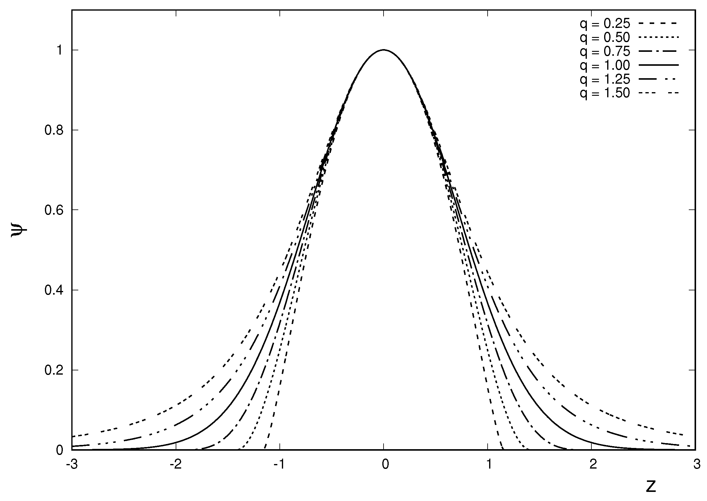
Figure 2.
Plot of against the wave amplitude ψ, for different q-values. The potential W is given by expression (17). All depicted quantities are dimensionless.
Figure 2.
Plot of against the wave amplitude ψ, for different q-values. The potential W is given by expression (17). All depicted quantities are dimensionless.
© 2017 by the authors. Licensee MDPI, Basel, Switzerland. This article is an open access article distributed under the terms and conditions of the Creative Commons Attribution (CC BY) license ( http://creativecommons.org/licenses/by/4.0/).
Share and Cite
MDPI and ACS Style
Plastino, A.R.; Wedemann, R.S. Nonlinear Wave Equations Related to Nonextensive Thermostatistics. Entropy 2017, 19, 60. https://doi.org/10.3390/e19020060
AMA Style
Plastino AR, Wedemann RS. Nonlinear Wave Equations Related to Nonextensive Thermostatistics. Entropy. 2017; 19(2):60. https://doi.org/10.3390/e19020060
Chicago/Turabian StylePlastino, Angel R., and Roseli S. Wedemann. 2017. "Nonlinear Wave Equations Related to Nonextensive Thermostatistics" Entropy 19, no. 2: 60. https://doi.org/10.3390/e19020060
Note that from the first issue of 2016, this journal uses article numbers instead of page numbers. See further details here.