Article

Classification of Normal and Pre-Ictal EEG Signals Using Permutation Entropies and a Generalized Linear Model as a Classifier

by
Francisco O. Redelico
1,
Francisco Traversaro
2,*,
María Del Carmen García
3,
Walter Silva
4,
Osvaldo A. Rosso
1,5,6 and
Marcelo Risk
1,2
1
Departamento de Informática en Salud, Hospital Italiano de Buenos Aires, C1199ABB Ciudad Autónoma de Buenos Aires, Argentina
2
Instituto Tecnológico de Buenos Aires (ITBA), C1106ACD Ciudad Autónoma de Buenos Aires, Argentina
3
Servicio de Neurología, Hospital Italiano de Buenos Aires, Gral. Juan Domingo Perón 4190, C1199ABB Ciudad Autónoma de Buenos Aires, Argentina
4
Servicio de Neurologia Infantil—Instituto Universitario (IUHI)—Hospital Italiano de Buenos Aires, Tte. Gral. Juan Domingo Perón 4190, C1199ABB Ciudad Autónoma de Buenos Aires, Argentina
5
Instituto de Física, Universidade Federal de Alagoas (UFAL), 57072-900 Maceió, Brazil
6
Complex Systems Group, Facultad de Ingeniería y Ciencias Aplicadas, Universidad de los Andes, 12455 Santiago, Chile
*
Author to whom correspondence should be addressed.
Entropy 2017, 19(2), 72; https://doi.org/10.3390/e19020072
Submission received: 17 November 2016 / Revised: 26 January 2017 / Accepted: 10 February 2017 / Published: 16 February 2017
(This article belongs to the Special Issue Entropy and Electroencephalography II)

Abstract

:
In this contribution, a comparison between different permutation entropies as classifiers of electroencephalogram (EEG) records corresponding to normal and pre-ictal states is made. A discrete probability distribution function derived from symbolization techniques applied to the EEG signal is used to calculate the Tsallis entropy, Shannon Entropy, Renyi Entropy, and Min Entropy, and they are used separately as the only independent variable in a logistic regression model in order to evaluate its capacity as a classification variable in a inferential manner. The area under the Receiver Operating Characteristic (ROC) curve, along with the accuracy, sensitivity, and specificity are used to compare the models. All the permutation entropies are excellent classifiers, with an accuracy greater than 94.5% in every case, and a sensitivity greater than 97%. Accounting for the amplitude in the symbolization technique retains more information of the signal than its counterparts, and it could be a good candidate for automatic classification of EEG signals.

1. Introduction

Epilepsy is a neurological condition in which patients suffer spontaneous seizures. The occurrence of two seizures with unknown idiopathic condition is necessary for the diagnosis of epilepsy. These seizures are caused by disturbances in the electrical activity of the brain. As was proposed by the International League Against Epilepsy (ILAE) and the International Bureau for Epilepsy (IBE), an epileptic seizure is a transient occurrence of signs and/or symptoms due to abnormal, excessive, and synchronous neuronal activity in the brain [1,2]. Epilepsy presents itself in seizures which result from abnormal hyper-synchronous brain activity. The sudden and often unforeseen occurrence of seizures represents one of the most disabling aspects of the disease. Correctly identifying the presence of epileptic activity, characterizing the spatio-temporal patterns of the corresponding brain activity, and predicting the occurrence of seizures are major challenges, and achieving this could significantly improve the quality of life for patients with epilepsy. The elapsed time between seizures in patients with epilepsy is called the inter-ictal period. This paper deals with the problem of classification between electroencephalogram (EEG) signals of seizure-free periods from patients with epilepsy and healthy persons, using several entropies based on a discrete probability distribution function derived from symbolization techniques.
Permutation entropy [3] has been used in several application to study brain (electrical) activity, namely in epilepsy research [4,5,6,7,8,9,10]—for example, for determinism detection and dynamical changes in EEG signals. Often, epileptic seizures manifest in highly stereotypical ordered sequences of symptoms and signs with limited variability, and for this reason, Schindler et al. [11] conjectured that this stereotype may imply that ictal neuronal dynamics might have a deterministic characteristic, and that this would presumably be enhanced in the ictogenic regions of the brain. Hence, for determinism detection in EEG signals, the permutation entropy was used in [10,12], among others. As for dynamical changes, accurate detection of transitions from normal to pathological states may improve diagnosis and treatment, so detection of dynamic change in EEG signals is important in clinical studies. In [4], permutation entropy was used to identify the various phases of epileptic activity in the intracranial EEG signals recorded from patients suffering from intractable epilepsy. Permutation entropy was also used in prediction and classification: [13] proved—for a population of rats—that permutation entropy can be used not only to track the dynamical changes of EEG data, but also to successfully detect pre-seizure states. The classification task is one prominent activity in epilepsy research [14] that is important for diagnostic purposes, as it allows discrimination between normal and pathological electroencephalographic records, which are often a nontrivial issue, and it is the task to cope in this contribution.
Renyi entropy [15] was used for classification purposes in [15], as it allows differentiation of the focal and non-focal EEG signals. In [16], the permutation min-entropy (i.e., the Renyi entropy with its probabilities estimates according de Bandt and Pompe methodology [3] and the α e x p o n e n t tending to infinity) was applied to discriminate between EEG signals of healthy volunteers and EEG signals from interictal periods of patients with epilepsy. Its discriminating power was compared with the usual permutation entropy in a descriptive manner.
Tsallis entropy was used in [17] in the study of human EEG-signal; it was shown that Tsallis non-extensive measures discriminate better than their Shannon counterparts.
Weighted permutation entropy (WPE) is presented in [18] and tested in Single Channel and Multichannel EEG Signals. In [19], three different EEG physiological states—eye-closed (EC), eye-open (EO), and visual oddball task (VOT)—were included in the study to examine the ability of WPE to identify and discriminate different physiological states. In the classification literature (in the context of machine learning), there exist several previous efforts to discriminate between EEG of healthy volunteers and EEG from interictal periods of patients with epilepsy; e.g., [20] uses a Recurrent neural network with time and frequency domain features, [21] use a decision tree combined with a Fast Fourier Transform, and [22] combined Discrete wavelet transform and a Mixture Expert Model. Regarding the use of entropies, [15] used an adaptive neuro fuzzy inference system endowed with entropies, [23] used Approximate Entropy and an Elman network. Most of them with high accuracy of separation between signals, more than 95% of signals were correctly classified.
The objective of the present contribution is to quantify the potential of permutation entropy and some related entropies as independent variables in a generalized linear model to discriminate between EEG records from healthy patients and from patients with epilepsy in a inferential framework. To our knowledge, aside from the mentioned machine learning approaches, no parametric models have been used with permutation entropies. The use of a logistic regression model will give new insights for classification purposes. The paper reads as follows: Section 2 briefly reviews the entropy-based quantifiers used as independent variables in the generalized linear model explained in Section 4. Section 3 presents the EEG database analyzed, and finally Section 5 is devoted to presenting the numerical results and discussion.

2. Brief Review on Permutation Entropy, Renyi Permutation Entropy, Min-Permutation Entropy, Weighted Permutation Entropy, and Tsallis Entropy

Given a continuous probability distribution function (PDF) f ( x ) with x Δ R and Δ f ( x ) d x = 1 , its associated Shannon Entropy S [24]
S [ f ] = Δ f ( x ) ln f ( x ) d x
is a measure of global character that it is not too sensitive to strong changes in the distribution taking place on a small-sized region. Let now P = { p i ; i = 1 , , N } , with i = 1 N p i = 1 , be a discrete probability distribution (PDF) with N the number of possible states of the system under study. In the discrete case, we define a “normalized” Shannon entropy ( 0 H 1 ) as
H [ P ] = S [ P ] / S m a x = i = 1 N p i ln ( p i ) / S m a x ,
where the denominator S m a x = S [ P e ] = ln N is that attained by a uniform probability distribution P e = { p i = 1 / N , i = 1 , , N } .
Bandt and Pompe introduced a successful methodology for the evaluation of the PDF associated with scalar time series data using a symbolization technique [3]. For a didactic description of the approach, as well as its main biomedical and econophysics applications, see [14]. To use the Bandt and Pompe [3] methodology for evaluating the PDF, P, associated with the time series (dynamical system) under study, one starts by considering partitions of the pertinent D-dimensional space that will hopefully “reveal” relevant details of the ordinal structure of a given one-dimensional time series X ( t ) = { x t ; t = 1 , , M } with embedding dimension D > 1 ( D N ) and time delay τ ( τ N ). We are interested in “ordinal patterns” of order (length) D generated by
( s ) x s ( D 1 ) τ , x s ( D 2 ) τ , , x s τ , x s ,
which assigns to each time s the D-dimensional vector of values at times s , s τ , , s ( D 1 ) τ . Clearly, the greater the D value, the more information on the past is incorporated into our vectors. By “ordinal pattern” related to the time ( s ) , we mean the permutation π = ( r 0 , r 1 , , r D 1 ) of [ 0 , 1 , , D 1 ] defined by
x s r D 1 τ x s r D 2 τ x s r 1 τ x s r 0 τ .
In order to get a unique result, we set r i < r i 1 if x s r i = x s r i 1 . This is justified if the values of x t have a continuous distribution, so that equal values are very unusual. Thus, for all the D ! possible permutations π of order D, their associated relative frequencies can be naturally computed by the number of times this particular order sequence is found in the time series divided by the total number of sequences,
p ( π ) = { s | s M D + 1 ; ( s ) , has type π } M D + 1 .
In this expression, the symbol ♯ stands for “number”.
Consequently, it is possible to quantify the diversity of the ordering symbols (patterns of length D) derived from a scalar time series by evaluating the so-called permutation entropy (Shannon entropy). Of course, the embedding dimension D plays an important role in the evaluation of the appropriate probability distribution, because D determines the number of accessible states D ! and also conditions the minimum acceptable length M D ! of the time series that one needs in order to work with reliable statistics [25]. Regarding the selection of the parameters, Bandt and Pompe suggested working with 3 D 6 , and specifically considered an embedding delay τ = 1 in their cornerstone paper [3]. Nevertheless, it is clear that other values of τ could provide additional information [26].
Renyi entropy, which generalizes Shannon Entropy, is defined as follows:
R α P = 1 1 α ln i = 1 D ! p i α ,
where the order α ( α 0 and α 1 ) is a bias parameter, and the Shannon entropy is recovered in the limit as α 1 . If the required p i are calculated using the Bandt & Pompe methodology, it leads to the permutation Renyi entropy [27].
Renyi entropy is linked to the probability distribution taken from the time series through α. High α emphasizes the super-Gaussian or leptokurtic distributions [28] (i.e., both a sharper peak and fatter tail than the corresponding Gaussian), whereas low-level α emphasizes the sub-Gaussian or platykurtic ones [29] (i.e., flatter peaks, thinner tail). Therefore, α can tune the sensitivity to the sub-Gaussianity, the super-Gaussianity of the BP-PDF distribution. Several special cases of α values are considered. When α 1 PE is recovered, and in the limit α , R α ( P ) converges to R ( P ) (i.e., the min-entropy).
R P = ln m a x i = 1 , , D ! p π i .
A variety of anomalous systems exist for which the powerful Boltzmann–Gibbs statistics formalism exhibits serious difficulties, as the long-range interacting systems [30], non-Markovian processes [31], among others. To deal with these systems, an attempt has been made in [32] by postulating a nonextensive entropy (Tsallis entropy).
S q = ( 1 i p i q ) 1 q ,
This Tsallis entropy endowed with probabilities calculated using the BP methodology is used in this contribution; in the limit q 1 , the Tsallis entropy converges to the Boltzmann–Gibbs statistics, recovering the permutation entropy.
All the permutation entropies considered above do not account for the amplitude of the time series, they are only aware about the relative order of the sample point within the series. In [18], a version of the PE dealing with the amplitude of the time series—named as weighted permutation entropy—is presented. This particular entropy weights each pattern according to the dispersion measure:
w j = 1 D k = 1 D x j + ( k 1 ) τ X ¯ j D , τ 2 ,
where X ¯ j D , τ stands for the mean value of the embedded vector of length D and time delay τ. Then the relative frequencies of each π is calculated as:
p w ( π ) = j M { s j | s j ,   has   type   π } w j k M s k w k
and the entropy is obtained as:
H w [ P ] = i = 1 N p i w ln ( p i w )

3. EEG Data

In order to illustrate the performance of the previously presented quantifiers in real contexts using logistic regression as the statistical model, we use free EEG time series data from the Department of Epileptology, University of Bonn [33], available at [34]. Two sets—A and B, each containing 200 single channel EEG segments of 23.6 sec duration—were recorded for the study. These segments were selected and cut out from continuous multichannel EEG recordings after visual inspection for artifacts (e.g., due to muscle activity or eye movements). Set A consisted of segments taken from surface EEG recordings that were carried out on five healthy volunteers, relaxed in an awake state. This sample will be referred to as normal within this paper. Set B was originated from an EEG archive of presurgical diagnosis during pre-ictal periods (i.e., periods when no seizure are detected in the epilepsy patient). This sample will be referred to as pre-ictal within this paper. Epileptic EEGs were collected from intracranial electrodes that were placed on the correct epileptogenic zone [33,35]. The data set consists of 400 data segments, 200 belonging the normal condition and 200 belonging to the pre-ictal condition, whose length is 4097 data points with a sampling frequency of 173.61 Hz for each group. These data were analysed for classification in a very different context—as artificial intelligence—in [36,37] among others, as well as in a information theory context [14] among others.

4. Classification Models

4.1. Logistic Regression

Logistic regression is the most popular method for predicting binary outcomes on the basis of one or more predictor variables, and the central mathematical concept that underlies logistic regression is the logit, the natural logarithm of an odds ratio. In the simplest case of linear regression for one continuous predictor X and one dichotomous outcome variable Y, the plot of such data results in two parallel lines, which are difficult to describe with an ordinary least square regression equation; it fits much better with an S-shaped curve (often referred to as sigmoidal). Applying the logit transformation to the dependent variable solves this fitting problem; it follows that the model does not require that the error should be normal or constant across the range of data. Given that the response variable Y is binary, we will describe it as a random variable on either the value 0 or the value 1, depending on whether the observation has an attribute present or not. For example, Y = 1 if the patient presents a certain illness, and Y = 0 otherwise. In a simple logistic regression equation with one predictor variable, X, we denote by ρ ( x ) the probability that the response variable Y equals 1 (the disease is present) given that X = x .
l o g i t ( Y ) = ln ρ 1 ρ = α + β x ,
ρ ( x ) = e α + β x 1 + e α + β x .
Where the value of the coefficient β determines the direction between X and the logit of Y. A test can be done where the null hypothesis states that β equals zero. Rejecting such a null hypothesis implies that a linear relationship exists between X and the logit of Y. If the predictor is binary, the interpretation of this coefficient is as follows:
ρ 1 ρ = P ( Y = 1 | X = x ) P ( Y = 0 | X = x ) = k e β x .
So, if the value of the variable X increases in one point, and the value of β is positive, the odds ratio increases in a factor of e β . Following the example, the odds ratio represents how probable it is that the patient is ill in relation with the probability that the patient does not have that illness. If the model has good forecasting properties, it can be used as a classification tool. A excellent method of testing the classification power of a logistic regression is the Receiver Operating Characteristic (ROC) curve.

4.2. ROC Curve: Classifier Performance

Initially, only a two-class classification process is considered. Each instance Y is mapped to one element of the set { P , N } , positive and negative class labels. A classification model (classifier) is a mapping from instances to predicted classes. As previously stated in Section 4.1, Logistic Regression can be an excellent classifier. Each instance Y, or observation, is either 1 or 0 (i.e., has the disease or not). The predictions produced by the model, ρ ( x ) , are continuous, so a threshold or a cut-off point ( c ) is needed to have a two-class classifier. If ρ ( x ) c , then Y is predicted as 1, and the prediction is 0 otherwise. To simplify, the prediction class is going to be in the set { P , N } .
Now, given a classifier and and instance, there are four possible outcomes: True Positive (TP) when the instance is positive and is classified as positive; False Negative (FN), the instance is positive and is classified as negative; False Positive (FP) the instance is negative and is classified as positive; and finally, True Negative (TN) when the instance is negative and is classified as negative. So, we define:
Sensitivity = T P T P + F N ,
Specificity = T N T N + F P .
Thus, sensibility reflects the power of the model to correctly identify the positive class, and the specificity is the power to identify the negative class. Another useful performance indicator for a given cut-off point ( c ) is the accuracy of the model, and is defined simply as the percentage of well-classified observations in the data set,
T P + T N N o b s ,
where N stands for the number of observations.
In a ROC curve, the sensitivity is plotted as a function of the false positive rate (1–Specificity) for different cut-off points. Each point on the ROC curve represents a sensitivity/specificity pair corresponding to a particular decision threshold. A test with perfect discrimination (no overlap in the two distributions) has a ROC plot that passes through the upper left corner (Specificity = 1 , Sensitivity = 1 ). This leads to the conclusion that the closer the ROC plot is to the upper left corner, the higher the overall accuracy of the test. As the ROC is a two-dimensional depiction of classifier performance, a single scalar value would be useful to compare classifiers. A common method is to calculate the area under the curve (AUC) [38]. Since the AUC is a portion of the area of the unit square, its area is going to be less than 1. Random guessing produces the line between ( 0 , 0 ) and ( 1 , 1 ) ; any realistic classifier should have an AUC greater than 0.5 . In general terms, any area between 0.8 and 0.9 stands for a good test, and any area between 0.9 and 1 represents an excellent test.

4.3. The Validation Set Approach: 10-Fold Cross-Validation

When the whole set of observations is used to estimate the desired indicator of classifier performance of the model (in this case, the AUC), over fitting occurs, and this performance indicator is overestimated. In order to avoid this, several methods were developed that consist of holding out a subset of testing observation from the fitting process, and then applying the model to those held-out observations to estimate the AUC. The method consists of randomly dividing the available set of observations into two parts: the training set and the validation set. The model is fit on the training set, and this fitted model is used on the validation set to the AUC or the test error rate. An improvement of this simple method is to divide the observation set in k-folds of approximately equal size, using the first k 1 folds to fit the model, and applying the fitted model to the remaining fold to estimate the AUC. Then, this methodology is repeated k times using each fold exactly one time as the validation set, and the rest as the training set. For each time, the estimated AUC is independent of the values used to fit the model. The average of this k values of the AUC (performance classifier) is the resulting overall AUC for the proposed model. Typical values of k are k = 5 and k = 10 . For this contribution, k = 10 is used.

5. Results and Discussion

To discriminate between normal and pre-ictal EEG signals, the methodology proposed by Hosmer and Lemeshow [39] is used. It is important to note that—unlike the reference articles in the Introduction Section—we use a parametric method of classification, leading to an interpretation of the estimated parameters, and we also gain an insight of the causal structure of the time series using the PDF Histogram using the BP methodology of the best combination to separate the signals. We perform a logistic regression model for each entropy (i.e., permutation entropy H ( P ) , weighted permutation entropy H w ( P ) , MinEntropy R P , Renyi Entropy R α P , and Tsallis Entropy S q P ) described in Section 2 as a explanatory variable to classify EEG signals as normal or pre-ictal. We evaluate each combination of pattern length D = { 3 , 4 , 5 , 6 } and time delay τ = { 1 , 2 , 3 , 4 , 5 } to calculate the entropies. For the Renyi entropy, we range the parameter α from 0.25 to 7.5 with 0.25 increments (following [27]), and for the Tsallis Entropy we range the parameter q from 0.1 to 3 with 0.1 increments [40]. In Figure 1, the area under ROC curve calculated by 10-fold cross-validation is plotted (AUC ± 1 sd) against the time delay τ. The figure is divided by the different entropies and by the embedding dimension D for better understanding. It reveals that—independent of the entropy used—the best model for classifying is when the discrete PDF is calculated for embedding dimension D = 3 and time delay τ = 5 , with the exception of the MinEntropy, since the model for D = 4 and τ = 4 is slightly better. When the time delay increases, all entropies perform better as a classifier distinguishing normal EEG signals from pre-ictal ones. In both Renyi Entropy R α P and Tsallis Entropy S q P , the influence of the parameter in the classification performance diminish as the τ augments, evidenced in the the decrement of the dispersion between the AUC values.
The permutation entropy H [ P ] as a classifier between normal and pre-ictal EEG signals has the strongest correlation with a β = 336 , with a p-value near to zero (Table 1). This means that for every 1 / 1000 the H [ P ] moves up, the odds ratio (the quotient between the probability of classifying the EEG signal as pre-ictal and the probability of classifying the EEG signal as normal) decreases by 28%. In other words, small increments on the H [ P ] significantly affects the probability of detecting pre-ictal states. Adding noise to a signal increases the permutation entropy, so noisy EEG signals would result in lower Sensitivity (i.e., the ability to detect pre-ictal EEG signals). On the other hand, MinEntropy R P has the weakest correlation with a β = 13.29 , meaning that for every 1 / 1000 the R P moves up, the odds ratio decreases only 1.2%, and it is still an excellent classifier. This behaviour in a classification model indicates robustness, because small increments in the value of the entropy does not affect the classification. This holds because all the entropies are on the same scale. The models with the highest (in absolute value) β coefficient have a more pronounced slope in the S-shaped curve, leading to a classification more sensible to changes. Figure 2 shows the five models presented in Table 1. The actual class of the observations are plotted as black circles. The curve in each plot represents the probability of the signal of being a pre-ictal EEG signal, according to the model, as a function of the value of the entropy. When this probability is larger than c = 0.5 , this observation is classified as pre-ictal EEG (blue crosses), and when it is less than c = 0.5 , as normal (red crosses). For all that is stated before, MinEntropy R P is the most robust model, followed by the model that uses weighted permutation entropy H w ( P ) .
These values of c can be changed according to each problem, so for purposes of comparison, the AUC is used because it accounts for all the possible values of c.
Table 1 presents the best models for each entropy, sorted by decreasing AUC. For the Renyi Entropy R α P and for the Tsallis Entropy S q P , the parameter is also chosen according to the classification performance (account for the fact that there is a model for each value of the parameter), that is Renyi Entropy with α = 2.75 and Tsallis Entropy with q = 1.1 . The entropy that has the best classification performance is the weighted permutation entropy, followed by the MinEntropy by less than a standard deviation, and the remaining entropies have similar performance in terms of the AUC (Figure 3). All the entropies have an excellent and similar performance in terms of Accuracy, so the overall classification error is small for the cut-off point c = 0.5 , and for this c, looking at the Specificity and the Sensitivity, all the models are more accurate classifying pre-ictal EEG signals as such than classifying normal EEG correctly.
The obtained AUC is the highest within the papers reviewed and noted in the Introduction Section. Using entropies endowed with the BP methodology for calculating the involved probabilities allows us to get an insight into the causal structure of the time series.
In summary, in this contribution, we compare the classification potential of several competing quantifiers: permutation entropy H ( P ) , weighted permutation entropy H w ( P ) , MinEntropy R P , Renyi Entropy R α P , and Tsallis Entropy S q P . All these quantifiers perform excellently. For this case, weighted permutation entropy H w ( P ) results in the best classifier, so taking account of the amplitude could improve the classification performance. However, as the differences between the AUC are not significant, some considerations should be done by the researcher in order to select one or the other entropy, as the noise or artifacts present in the signal. MinEntropy R P is more robust against noise than permutation entropy H ( P ) , as shown in [16]; this can be very useful in the presence of EEG with noise. The weighted permutation entropy H w ( P ) retains more information of the signal than its counterparts, and it could be a good candidate for automatic classification of EEG signals.

Acknowledgments

FOR, OAR and MR gratefully acknowledge financial support from Consejo Nacional de Investigaciones Científicas y Técnicas (CONICET), Argentina.

Author Contributions

Francisco O. Redelico and Osvaldo A. Rosso conceived the study, María del Carmen García, Walter Siva and Marcelo Risk gave technical support and conceptual advice. Francisco O. Redelico and Francisco Traversaro analyzed the data, wrote the paper and performed the statistical analysis. All authors discussed the results and implications and commented on the manuscript at all stages. All authors have read and approved the final manuscript.

Conflicts of Interest

The authors declare no conflict of interest.

References

  1. Fisher, R.S.; Boas, W.E.; Blume, W.; Elger, C.; Genton, P.; Lee, P.; Engel, J. Epileptic seizures and epilepsy: Definitions proposed by the International League Against Epilepsy (ILAE) and the International Bureau for Epilepsy (IBE). Epilepsia 2005, 46, 470–472. [Google Scholar] [CrossRef] [PubMed]
  2. Fisher, R.S.; Acevedo, C.; Arzimanoglou, A.; Bogacz, A.; Cross, J.H.; Elger, C.E.; Engel, J.; Forsgren, L.; French, J.A.; Glynn, M.; et al. ILAE official report: A practical clinical definition of epilepsy. Epilepsia 2014, 55, 475–482. [Google Scholar] [CrossRef] [PubMed]
  3. Bandt, C.; Pompe, B. Permutation entropy: A natural complexity measure for time series. Phys. Rev. Lett. 2002, 88, 174102. [Google Scholar] [CrossRef] [PubMed]
  4. Cao, Y.; Tung, W.; Gao, J.; Protopopescu, V.A.; Hively, L.M. Detecting dynamical changes in time series using the permutation entropy. Phys. Rev. E 2004, 70, 046217. [Google Scholar] [CrossRef] [PubMed]
  5. Keller, K.; Wittfeld, K. Distances of time series components by means of symbolic dynamics. Int. J. Bifurc. Chaos 2004, 14, 693–703. [Google Scholar] [CrossRef]
  6. Veisi, I.; Pariz, N.; Karimpour, A. Fast and robust detection of epilepsy in noisy EEG signals using permutation entropy. In Proceedings of the 2007 IEEE 7th International Symposium on BioInformatics and BioEngineering, Boston, MA, USA, 14–17 October 2007; pp. 200–203.
  7. Li, X.; Ouyang, G.; Richards, D.A. Predictability analysis of absence seizures with permutation entropy. Epilepsy Res. 2007, 77, 70–74. [Google Scholar] [CrossRef] [PubMed]
  8. Ouyang, G.; Li, X.; Dang, C.; Richards, D.A. Deterministic dynamics of neural activity during absence seizures in rats. Phys. Rev. E 2009, 79, 041146. [Google Scholar] [CrossRef] [PubMed]
  9. Ouyang, G.; Dang, C.; Richards, D.A.; Li, X. Ordinal pattern based similarity analysis for EEG recordings. Clin. Neurophysiol. 2010, 121, 694–703. [Google Scholar] [CrossRef] [PubMed]
  10. Bruzzo, A.A.; Gesierich, B.; Santi, M.; Tassinari, C.A.; Birbaumer, N.; Rubboli, G. Permutation entropy to detect vigilance changes and preictal states from scalp EEG in epileptic patients. A preliminary study. Neurol. Sci. 2008, 29, 3–9. [Google Scholar] [CrossRef] [PubMed]
  11. Schindler, K.; Gast, H.; Stieglitz, L.; Stibal, A.; Hauf, M.; Wiest, R.; Mariani, L.; Rummel, C. periictal intracranial EEG indicate deterministic dynamics in human epileptic seizures. Epilepsia 2011, 53, 225. [Google Scholar]
  12. Nicolaou, N.; Georgiou, J. Detection of epileptic electroencephalogram based on permutation entropy and support vector machines. Expert Syst. Appl. 2012, 39, 202–209. [Google Scholar] [CrossRef]
  13. Li, H.; Heusdens, R.; Muskulus, M.; Wolters, L. Analysis and synthesis of pseudo-periodic job arrivals in grids: A matching pursuit approach. In Proceedings of the Seventh IEEE International Symposium on Cluster Computing and the Grid (CCGrid’07), Rio de Janeiro, Brazil, 14–17 May 2007; pp. 183–196.
  14. Zanin, M.; Zunino, L.; Rosso, O.A.; Papo, D. Permutation entropy and its main biomedical and econophysics applications: A review. Entropy 2012, 14, 1553–1577. [Google Scholar] [CrossRef]
  15. Kannathal, N.; Choo, M.L.; Acharya, U.R.; Sadasivan, P. Entropies for detection of epilepsy in EEG. Comput. Methods Programs Biomed. 2005, 80, 187–194. [Google Scholar] [CrossRef] [PubMed]
  16. Zunino, L.; Olivares, F.; Rosso, O.A. Permutation min-entropy: An improved quantifier for unveiling subtle temporal correlations. EPL (Europhys. Lett.) 2015, 109, 10005. [Google Scholar] [CrossRef]
  17. Capurro, A.; Diambra, L.; Lorenzo, D.; Macadar, O.; Martín, M.; Mostaccio, C.; Plastino, A.; Perez, J.; Rofman, E.; Torres, M.; et al. Human brain dynamics: the analysis of EEG signals with Tsallis information measure. Physica A 1999, 265, 235–254. [Google Scholar] [CrossRef]
  18. Fadlallah, B.; Chen, B.; Keil, A.; Principe, J. Weighted-permutation entropy: A complexity measure for time series incorporating amplitude information. Phys. Rev. E 2013, 87, 022911. [Google Scholar] [CrossRef] [PubMed]
  19. Vuong, P.L.; Malik, A.S.; Bornot, J. Weighted-permutation entropy as complexity measure for electroencephalographic time series of different physiological states. In Proceedings of the 2014 IEEE Conference on Biomedical Engineering and Sciences (IECBES), Kuala Lumpur, Malaysia, 8–10 December 2014; pp. 979–984.
  20. Srinivasan, V.; Eswaran, C.; Sriraam, N. Artificial neural network based epileptic detection using time-domain and frequency-domain features. J. Med. Syst. 2005, 29, 647–660. [Google Scholar] [CrossRef] [PubMed]
  21. Polat, K.; Güneş, S. Classification of epileptiform EEG using a hybrid system based on decision tree classifier and fast Fourier transform. Appl. Math. Comput. 2007, 187, 1017–1026. [Google Scholar] [CrossRef]
  22. Subasi, A. EEG signal classification using wavelet feature extraction and a mixture of expert model. Expert Syst. Appl. 2007, 32, 1084–1093. [Google Scholar] [CrossRef]
  23. Ocak, H. Automatic detection of epileptic seizures in EEG using discrete wavelet transform and approximate entropy. Expert Syst. Appl. 2009, 36, 2027–2036. [Google Scholar] [CrossRef]
  24. Shannon, C.E. Communication theory of secrecy systems. Bell Syst. Tech. J. 1949, 28, 656–715. [Google Scholar] [CrossRef]
  25. Rosso, O.A.; Larrondo, H.; Martin, M.; Plastino, A.; Fuentes, M. Distinguishing noise from chaos. Phys. Rev. Lett. 2007, 99, 154102. [Google Scholar] [CrossRef] [PubMed]
  26. Zunino, L.; Soriano, M.C.; Rosso, O.A. Distinguishing chaotic and stochastic dynamics from time series by using a multiscale symbolic approach. Phys. Rev. E 2012, 86, 046210. [Google Scholar] [CrossRef] [PubMed]
  27. Mammone, N.; Duun-Henriksen, J.; Kjaer, T.W.; Morabito, F.C. Differentiating Interictal and Ictal States in Childhood Absence Epilepsy through Permutation Rényi Entropy. Entropy 2015, 17, 4627–4643. [Google Scholar] [CrossRef]
  28. Parent, A.; Morin, M.; Lavigne, P. Propagation of super-Gaussian field distributions. Opt. Quantum Electron. 1992, 24, S1071–S1079. [Google Scholar] [CrossRef]
  29. Benveniste, A.; Goursat, M.; Ruget, G. Robust identification of a nonminimum phase system: Blind adjustment of a linear equalizer in data communications. IEEE Trans. Autom. Control 1980, 25, 385–399. [Google Scholar] [CrossRef]
  30. Pavón, D. Thermodynamics of superstrings. Gen. Relativ. Gravit. 1987, 19, 375–381. [Google Scholar] [CrossRef]
  31. Cáceres, M.O. Non-Markovian processes with long-range correlations: Fractal dimension analysis. Braz. J. Phys. 1999, 29, 125–135. [Google Scholar] [CrossRef]
  32. Tsallis, C. Possible generalization of Boltzmann-Gibbs statistics. J. Stat. Phys. 1988, 52, 479–487. [Google Scholar] [CrossRef]
  33. Andrzejak, R.G.; Lehnertz, K.; Mormann, F.; Rieke, C.; David, P.; Elger, C.E. Indications of nonlinear deterministic and finite-dimensional structures in time series of brain electrical activity: Dependence on recording region and brain state. Phys. Rev. E 2001, 64, 061907. [Google Scholar] [CrossRef] [PubMed]
  34. Available online: http://www.meb.unibonn.de/epileptologie/science/physik/eegdata.html (accessed on 16 February 2017).
  35. Andrzejak, R.; Widman, G.; Lehnertz, K.; Rieke, C.; David, P.; Elger, C. The epileptic process as nonlinear deterministic dynamics in a stochastic environment: An evaluation on mesial temporal lobe epilepsy. Epilepsy Res. 2001, 44, 129–140. [Google Scholar] [CrossRef]
  36. Acharya, U.R.; Molinari, F.; Sree, S.V.; Chattopadhyay, S.; Ng, K.H.; Suri, J.S. Automated diagnosis of epileptic EEG using entropies. Biomed. Signal Process. Control 2012, 7, 401–408. [Google Scholar] [CrossRef]
  37. Ghosh-Dastidar, S.; Adeli, H. A new supervised learning algorithm for multiple spiking neural networks with application in epilepsy and seizure detection. Neural Netw. 2009, 22, 1419–1431. [Google Scholar] [CrossRef] [PubMed]
  38. Bradley, A.P. The use of the area under the ROC curve in the evaluation of machine learning algorithms. Pattern Recognit. 1997, 30, 1145–1159. [Google Scholar] [CrossRef] [Green Version]
  39. Hosmer, D.W., Jr.; Lemeshow, S.; Sturdivant, R.X. Applied Logistic Regression; John Wiley & Sons: New York, NY, USA, 2013; Volume 398. [Google Scholar]
  40. Plastino, A.; Rosso, O.A. Entropy and statistical complexity in brain activity. Europhys. News 2005, 36, 224–228. [Google Scholar] [CrossRef]
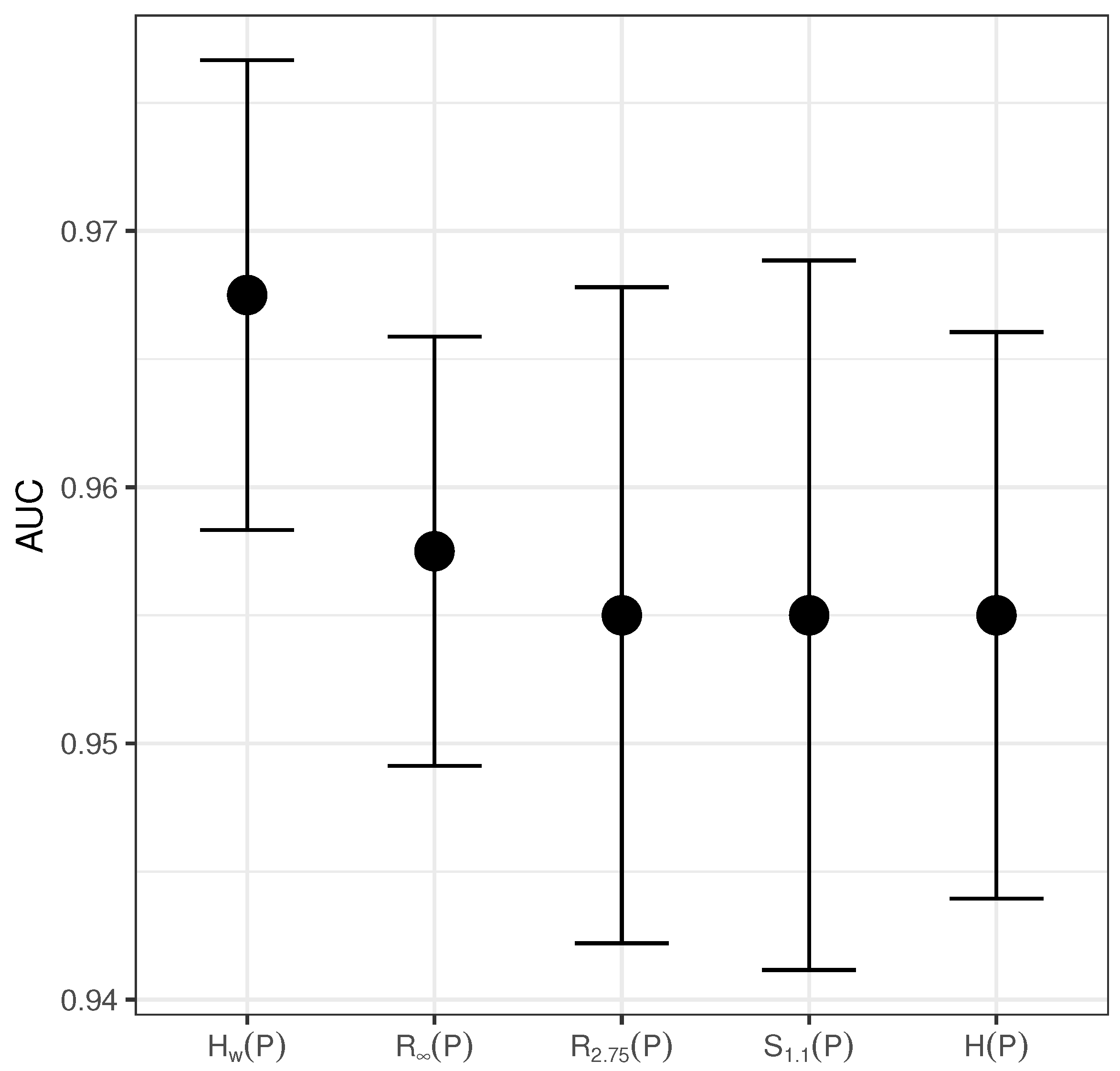
Figure 1. Area under Receiver Operating Characteristic (ROC) curve calculated by 10-fold cross-validation is plotted (area under the curve (AUC) ± 1 sd) against the time delay τ. The figure is divided by the different entropies and by the embedding dimension D for better understanding. It reveals that—independent of the entropy used—the best model for classifying is when the discrete Probability Distribution Function PDF is calculated for embedding dimension D = 3 and time delay τ = 5 , with the exception of the MinEntropy that the model for D = 4 and τ = 4 is slightly better, but with no significant difference.
Entropy 19 00072 g001
Figure 2. Shows the five logistic models presented in Table 1, with the explanatory variable in the x-axis (the different entropies), and the y-axis represents the probability that the signal is a pre-ictal EEG signal, so the curve in each plot represents the probability of the signal of being a pre-ictal EEG signal, according to the model, as a function of the value of the entropy. When this probability is larger than c = 0.5 , this observation is classified as pre-ictal EEG (blue crosses), and when it is less than c = 0.5 , as normal (red crosses). The actual class of the observations are plotted as black circles. The models with the highest (in absolute value) β coefficient have a more pronounced slope in the S-shaped curve, leading to a classification more sensible to changes. The permutation entropy H [ P ] as a classifier between normal and pre-ictal EEG signals has the strongest correlation with a β = 336 , with a p-value near to zero (Table 1). This means that for every 1 / 1000 the H [ P ] moves up, the odds ratio (the quotient between the probability of being ill and the probability of not having the disease) decreases by 28%. In other words, small increments on the H [ P ] significantly affects the probability of detecting the presence of the illness. Adding noise to a signal increases the permutation entropy, so noisy EEG signals would result in lower Sensitivity (i.e., the ability to detect pre-ictal EEG signals). On the other hand, MinEntropy R P has the weakest correlation with a β = 13.29 , meaning that for every 1 / 1000 the R P moves up, the odds ratio decreases by only 1.2%, and still is an excellent classifier. This behaviour in a classification model indicates robustness, because small increments in the value of the entropy do not affect the classification. This holds because all the entropies are on the same scale. MinEntropy R P is the most robust model, followed by the model that uses weighted permutation entropy H w ( P ) .
Entropy 19 00072 g002
Figure 3. The entropy that has the best classification performance is the weighted permutation entropy, followed by the MinEntropy by less than a standard deviation, and the remaining entropies have similar performance in terms of the AUC.
Entropy 19 00072 g003
Table 1. The best models for each entropy, sorted by decreasing AUC. For the Renyi Entropy R α P and for the Tsallis Entropy S q P , the parameter is chosen also according to the best classification performance (taking account that there is a model for each value of the parameter); that is, Renyi Entropy with α = 2.75 and Tsallis Entropy with q = 1.1 . The entropy that has the best classification performance is the weighted permutation entropy followed by the MinEntropy by less than a standard deviation, and the remaining entropies have similar performance in terms of the AUC. All the entropies have an excellent and similar performance in terms of Accuracy, so the overall classification error is small for the cut-off point c = 0.5 , and for this c, looking at the Specificity and the Sensitivity, all the models are more accurate classifying pre-ictal EEG signals as such than classifying normal EEG correctly.
EntropyAUCAccuracySensitivitySpecificityRegression
Coeficient
p-Value
H w ( P ) 0.96750.970.9850.95 107.98 3.57 × 10 13
R P 0.95750.9650.9750.94 13.298 1.86 × 10 12
H ( P ) 0.9550.9500.9750.935 335.99 2.76 × 10 12
R α P 0.9550.9500.970.94 121.78 1.26 × 10 12
S q P 0.9550.9450.970.94 203.07 2.78 × 10 12

