Pairs Generating as a Consequence of the Fractal Entropy: Theory and Applications

Abstract

In classical concepts, theoretical models are built assuming that the dynamics of the complex system’s stuctural units occur on continuous and differentiable motion variables. In reality, the dynamics of the natural complex systems are much more complicated. These difficulties can be overcome in a complementary approach, using the fractal concept and the corresponding non-differentiable theoretical model, such as the scale relativity theory or the extended scale relativity theory. Thus, using the last theory, fractal entropy through non-differentiable Lie groups was established and, moreover, the pairs generating mechanisms through fractal entanglement states were explained. Our model has implications in the dynamics of biological structures, in the form of the “chameleon-like” behavior of cholesterol.

1. Introduction

The dynamics of complex systems [1,2], from functionality and structure points of view, lead to some instabilities. These instabilities involve either chaos (e.g., noise regeneration) or pattern generation (e.g., interference, diffraction fields, etc.).

In classical concepts, the theoretical models (hydrodynamic, kinetic, etc. [1,3,4]) are built assuming that the dynamics of the complex system’s structural units occur on continuous and differentiable motion variables (energy, momentum, density, etc.), exclusively dependent on spatial coordinates and time.

In reality, the complex system’s dynamics are much more complicated and the classical theoretical models failed in the attempt to explain all these aspects, as illustrated by experimental observations [4].

These difficulties can be overcome with a complementary approach, using fractal concepts, which were defined for the first time by Mandelbrot [5]. He introduced the term “fractal” to describe the “exotic” shapes that did not fit the patterns of Euclidean geometry, i.e., irregular geometrical objects, cells of living organisms, human arterial vessels, neural networks, the convoluted surface of the brain, etc., which possess invariance with respect to the scale transformations. This approach is considered an extension of the conventional Euclidean geometry.

In this spirit, fractal analysis has proven to be a useful tool describing various systems from physics, chemistry, biology, medicine, etc. [6,7,8,9]. Moreover, the analysis of complex systems evolution showed that most of them are non-linear and, therefore, new mathematical tools were required. These have been provided by the scale relativity theory (SRT) [10,11] and by the extended scale relativity theory (ESRT) [12], i.e., the SRT with an arbitrary constant fractal dimension.

These theories consider that the motions of the complex system’s structural units take place on continuous but non-differentiable curves (fractal curves). In this situation, the Euclidean dynamics of a complex system subjected to external constraints is replaced by fractal dynamics characterizing the same system, but free of any external constraints. More precisely, the constrained motions in the Euclidian space, i.e., on continuous and differentiable curves, are substituted by free, independent motions (without constrains) in a fractal space, i.e., on continuous, but non-differentiable (fractal) curves.

Therefore, non-differentiability becomes a fundamental property of the complex system’s dynamics. In such a conjecture, a correspondence between the interaction processes and the non-differentiability (fractality) of the motion trajectories can be established. Then, for specific scales that are large with respect to the inverse of the highest Lyapunov exponent [13,14], the deterministic trajectories are replaced by a collection of potential trajectories, while the concept of definite positions is substituted by that of the probability density. Moreover, the complex system’s structural units may be reduced and identified with their own trajectories so that the complex system will behave as a special fluid lacking interactions (via their geodesics in a fractal space). Let us call such a fluid a “fractal fluid”.

In the present paper, the role of fractal entropy in the pairs generating processes is analyzed. The general theory and some applications are also discussed.

2. Hallmarks of Non-Differentiability

In such a framework, some consequences of non-differentiability, both in the usual space (of the space and time coordinates) and in the scales space, are evident [10,11,12,15,16,17]:

(i)

any continuous but non-differentiable curve of the complex system’s structural units (fractal curve) is explicitly dependent on scale resolution $\delta \omega$, i.e., its length tends to infinity when $\delta \omega$ tends to zero;

(ii)

the physics of the complex system phenomena is related to the behavior of a functions set during the zoom operation of the scale $\delta \omega$. Then, through the substitution principle, $\delta \omega$ will be identified with $d\omega$, i.e., $\delta \omega =d\omega$. Consequently, it will be considered as an independent variable;

(iii)

the complex system dynamics is described through fractal variables, i.e., functions dependent both on the space-time coordinates and the scale resolution, since the differential reflection invariance in relation to $\omega$, of any dynamical variable, is broken.

As consequence, the velocity field, both in the usual space and in the scales space, becomes a complex variable dynamic, with the form:

$$\stackrel{\wedge }{V^l}=V_D^l-i{V}_F^l, i=\sqrt{-1}$$

(1)

where the real part, $V_D^l$, is the differentiable velocity and the imaginary one, $V_F^l$, is the non-differentiable (fractal) velocity;

(iv)

the differential of the spatial coordinate field, $d_{\pm }{Y}^i$, both in the usual space and in the scales space, is expressed as the sum of two differentials, one of them being the differential part $d_{\pm }{y}^i$ and the other one being the scales fractal part, $d_{\pm }{\sigma }^i$, i.e.,:

$$d_{\pm }{Y}^i=d_{\pm }{y}^i+d_{\pm }{\sigma }^i$$

(2)

The sign “+” corresponds to the forward process, while the sign “−” to the backward one;

(v)

the fractal part of the spatial coordinate field, both in the usual space and in the scales space, satisfies the fractal equation:

$$d_{\pm }{\sigma }^i\left(\omega ,d\omega \right)={\lambda }_{\pm }^i{\left(d\omega \right)}^{1/D_F}$$

(3)

where $D_F$ defines the fractal dimension of the fractal motion curve and ${\lambda }_{\pm }^i$ are constant coefficients that indicate the fractalization type;

(vi)

an infinite number of fractal curves can be found relating any pair of points, both in the usual space and in the scales space. Then, any external constraint is interpreted as a selection of fractal curves, both in the usual space and in the scales space, and the real curves, corresponding to the maximum of the probability density;

(vii)

the complex system dynamics, both in the usual space and in the scales space, can be described through a covariant derivative:

$$\frac{\stackrel{\wedge }{d}}{d\omega }={\partial }_{\omega }+\stackrel{\wedge }{V^l}{\partial }_l-\frac{1}{4}{\left(d\omega \right)}^{\left(2/D_F\right)-1}{D}^{lk}{\partial }_l{\partial }_k$$

(4)

where:

$$\begin{array}{l}{D}^{lk}=\left({\lambda }_{+}^l{\lambda }_{+}^k-{\lambda }_{-}^l{\lambda }_{-}^k\right)-i({\lambda }_{+}^l{\lambda }_{+}^k+{\lambda }_{-}^l{\lambda }_{-}^k)\\ {\partial }_l=\frac{\partial }{\partial Y^l};{\partial }_l{\partial }_k=\frac{{\partial }^2}{\partial Y^l\partial Y^k}\end{array}$$

(5)

In the previous relations the indexes $l,k$ take the values $1,2,3$ in the usual space, while in the scales space they have an arbitrary dimension imposed by the intrinsic structure of the complex system.

Considering the functionality of a generalized covariance principle (the complex system physics laws are invariant both with respect to space-time transformations and to the scales ones), the transition from the classical physics of complex system dynamics to the non-differentiable (fractal) one can be implemented by replacing the standard derivative operator $d/d\omega$ with the non-differentiable operator $\frac{\stackrel{\wedge }{d}}{d\omega }$. Thus, this operator plays the role of the covariant derivative, namely it is used to rewrite the fundamental equations of complex system dynamics, both in the usual space and in the scales space, in the same form as in the classic (differentiable) case.

Under these conditions, applying the operator (4) to the complex velocity field (1), in the absence of any external constraint and for motions on Levy curves [5,6,7], which implies the restriction:

$${\lambda }_{+}^i{\lambda }_{+}^l=-{\lambda }_{-}^i{\lambda }_{-}^l=\pm 2\lambda {\delta }^{il}$$

(6)

where $\lambda$ is the fractal-nonfractal transition coefficient, considered with “+” for $d\omega \rangle 0$ and with “−” for $d\omega \langle 0$ (for details see [10,11,12,15,16,17]) and ${\delta }^{il}$ the Kronecker tensor, the fractal equation of the motion (geodesics equation) has the following form:

$$\frac{\stackrel{\wedge }{d}\stackrel{\wedge }{V^i}}{d\omega }={\partial }_{\omega }\stackrel{\wedge }{V^i}+\stackrel{\wedge }{V^l}{\partial }_l\stackrel{\wedge }{V^i}-i\lambda {\left(d\omega \right)}^{\left(2/D_F\right)-1}{\partial }^l{\partial }_l\stackrel{\wedge }{V^i}$$

(7)

Previous results show that, both in the usual space and in the scales space, the local “acceleration”, the ”convection” and the “dissipation” make their balance at any point of the non-differentiable curve. Moreover, the presence of the complex viscosity-type coefficient indicates that the complex system is a rheological medium.

For irrotational motions, the complex velocity field $\stackrel{\wedge }{V^i}$ takes the form:

$$\stackrel{\wedge }{V^i}=-2i\lambda {\left(d\omega \right)}^{\left(2/D_F\right)-1}{\partial }^{i}ln\mathrm{\Psi }$$

(8)

Then substituting this relation in Equation (7), the geodesics equation, both in the usual space and in the scales space, becomes:

$${\lambda }^2{\left(d\omega \right)}^{\left(4/D_F\right)-2}{\partial }^l{\partial }_l\mathrm{\Psi }+i\lambda {\left(d\omega \right)}^{\left(2/D_F\right)-1}{\partial }_{\omega }\mathrm{\Psi }=0$$

(9)

In the previous Equations (8) and (9), $\mathit{ln}\mathrm{\Psi }$ is the scalar potential of the complex velocity field. As the geodesics Equation (15) is of a fractal Schrödinger type, the function $\mathrm{\Psi }$, through $\rho ={\left|\mathrm{\Psi }\right|}^2$, becomes a density probability, thus motivating the procedure for deterministic trajectories substitution with “potential trajectories collection”, i.e., the probability densities.

Moreover, if $\mathrm{\Psi }=\sqrt{\rho }\exp \left(iS\right)$ with $\sqrt{\rho }$ is the amplitude and $S$ is the phase of $\mathrm{\Psi }$, the complex velocity field has the real part:

$$V_D^i=2\lambda {\left(d\omega \right)}^{\left(2/D_F\right)-1}{\partial }^{i}S$$

(10)

and the imaginary one:

$$V_F^i=\lambda {\left(d\omega \right)}^{\left(2/D_F\right)-1}{\partial }^i\mathit{ln}\rho$$

(11)

Substituting Equation (1) with Equations (10) and (11) in Equation (7) and separating the real and the imaginary parts, up to an arbitrary phase factor which may be set to zero by a suitable choice of the phase of $\mathrm{\Psi }$, we obtained:

$${\partial }_{\omega }{V}_D^i+\left(V_D^l{\partial }_l\right)V_D^i=-{\partial }^{i}Q$$

(12)

$${\partial }_{\omega }\rho +{\partial }^i\left(\rho V_D^i\right)=0$$

(13)

where $Q$ is the specific fractal potential:

$$Q=-2{\lambda }^2{\left(d\omega \right)}^{\left(4/D_F\right)-2}\frac{{\partial }^l{\partial }_l\sqrt{\rho }}{\sqrt{\rho }}=-\frac{V_F^l{V}_{Fl}}{2}-\lambda {\left(d\omega \right)}^{\left(2/D_F\right)-1}{\partial }_i{V}_F^i$$

(14)

Equation (12) represents the specific momentum conservation law, while Equation (13) represents the states density conservation law. These equations define the fractal hydrodynamical model both in the usual space and in the scales space.

From such a perspective, the non-linear interactions between the structural units of the complex system induce a “fractal medium”; therefore, every structural unit is in a perpetual “interaction” with the “fractal medium”. The “fractal medium” dynamics are described by the fractal hydrodynamics equations, i.e., by the momentum and states density conservation laws.

The specific fractal potential is, at the same time, both a measure of the interaction degree between the structural unit and the fractal medium, as well as of the motion curves fractality. The fractal velocity field does not represent actual motion, but contributes to the transfer of the specific momentum and energy. This may be seen clearly from the absence of this velocity from the states density conservation law.

Any interpretation of the specific fractal potential should take cognizance of the “self” nature of the specific momentum transfer. While the standard energies are stored both in the form of the mass motion (kinetic energy) and potential energy, some is available elsewhere and only the total energy is conserved. It is the conservation of the total energy and momentum that ensures “fractal reversibility” and the existence of the fractal eigenstates, but denies a Levy motion fractal force of interaction with the “fractal medium”.

3. Fractal Entropy through Non-Differentiable Lie’s Group

Working with a variant of the Schrodinger-type geodesics equation (see Equation (9)), it implies that to each dynamic variable ${\Theta }_i$, a fractal operator can be associated $\stackrel{\wedge }{{\Theta }_i}$. This leads us to fractal differential equations with eigenfunctions and eigenvalues [10,11,12]. For example, the fractal operator of the angular momentum is given by the equation [10,11,12]:

$$\stackrel{\wedge }{L}=\stackrel{\wedge }{r}\times \stackrel{\wedge }{P}=-i\lambda {(dt)}^{(2/D_F)-1}\left(\stackrel{\wedge }{r}\times \nabla \right)$$

(15)

where $\stackrel{\wedge }{r}$, $\stackrel{\wedge }{P}$ are the fractal position-type and, specific momentum-type (the momentum of the mass unit) operators, respectively.

Thus, Equation (15) becomes:

$$\begin{array}{l}\stackrel{\wedge }{M_1}=-i\lambda {(dt)}^{(2/D_F)-1}\left(Y_2\frac{\partial }{\partial Y_3}-Y_3\frac{\partial }{\partial Y_2}\right)\\ \stackrel{\wedge }{M_2}=-i\lambda {(dt)}^{(2/D_F)-1}\left(Y_3\frac{\partial }{\partial Y_1}-Y_1\frac{\partial }{\partial Y_3}\right)\\ \stackrel{\wedge }{M_3}=-i\lambda {(dt)}^{(2/D_F)-1}\left(Y_1\frac{\partial }{\partial Y_2}-Y_2\frac{\partial }{\partial Y_1}\right)\end{array}$$

(16)

These non-diferentiable operators satisfy the Lie fractal algebra [10,11,12]:

$$\begin{gathered} \left[\stackrel{\wedge }{M_1},\stackrel{\wedge }{M_2}\right]=i\lambda {(dt)}^{(2/D_F)-1}\stackrel{\wedge }{L_3} \\ \left[\stackrel{\wedge }{M_2},\stackrel{\wedge }{M_3}\right]=i\lambda {(dt)}^{(2/D_F)-1}\stackrel{\wedge }{L_1} \\ \left[\stackrel{\wedge }{M_3},\stackrel{\wedge }{M_1}\right]=i\lambda {(dt)}^{(2/D_F)-1}\stackrel{\wedge }{L_2} \end{gathered}$$

(17)

and they make invariant the norm of the null vectors [10,11,12]:

$$Y_1^2+Y_2^2+Y_3^2=0$$

(18)

In the coordinates system:

$$Y_1=\rho \mathit{sin}\omega , Y_2=-\rho \mathit{cos}\omega , Y_3=-i\rho$$

(19)

and neglecting the fractality degree $\lambda {(dt)}^{(2/D_F)-1}$, operators (16) take the form:

$$\begin{array}{l}\stackrel{\wedge }{M_1}=\mathit{cos}\omega \cdot \rho \frac{\partial }{\partial \rho }-\mathit{sin}\omega \cdot \frac{\partial }{\partial \omega }\\ \stackrel{\wedge }{M_2}=\mathit{sin}\omega \cdot \rho \frac{\partial }{\partial \rho }+\mathit{cos}\omega \cdot \frac{\partial }{\partial \omega }\\ \stackrel{\wedge }{M_3}=-i\frac{\partial }{\partial \omega }\end{array}$$

(20)

Now, the action of the operators (20) on the spin-type fractal “eigenfunctions”:

$$v_{+}=\sqrt{\rho }{e}^{\frac{i\omega }{2}}, v_{-}=\sqrt{\rho }{e}^{-\frac{i\omega }{2}}$$

(21)

reproduces the action of the Pauli matrices, according to relations:

$$\begin{array}{l}\left[\begin{array}{cc}\stackrel{\wedge }{M_1}& v_{+}\\ \stackrel{\wedge }{M_1}& v_{-}\end{array}\right]=\frac{1}{2}\left[\begin{array}{cc}0& 1\\ 1& 0\end{array}\right]\left[\begin{array}{c}{v}_{+}\\ v_{-}\end{array}\right]\\ \left[\begin{array}{cc}\stackrel{\wedge }{M_2}& v_{+}\\ \stackrel{\wedge }{M_2}& v_{-}\end{array}\right]=\frac{1}{2}\left[\begin{array}{cc}0& i\\ -i& 0\end{array}\right]\left[\begin{array}{c}{v}_{+}\\ v_{-}\end{array}\right]\\ \left[\begin{array}{cc}\stackrel{\wedge }{M_3}& v_{+}\\ \stackrel{\wedge }{M_3}& v_{-}\end{array}\right]=\frac{1}{2}\left[\begin{array}{cc}-1& 0\\ 0& 1\end{array}\right]\left[\begin{array}{c}{v}_{+}\\ v_{-}\end{array}\right]\end{array}$$

(22)

It can be shown, in a “strange” manner, that the operators (20) satisfy the same algebras as Pauli’s matrices.

The infinitesimal operators (16) and (20) do not tell us very much about this group. In this respect, we shall set operators (20) in a form capable of putting into evidence its isomorphism to known groups [18,19].

The new operators are given by the linear combinations:

$$\stackrel{\wedge }{L_1}=\stackrel{\wedge }{M_1}-i\stackrel{\wedge }{M_2}, \stackrel{\wedge }{L_2}=\stackrel{\wedge }{M_3}, \stackrel{\wedge }{L_3}=-(\stackrel{\wedge }{M_1}+i\stackrel{\wedge }{M_2})$$

(23)

Taking $\alpha$ and $\overline{\alpha }$ as group variables, with $\alpha =v_{+}$ and $\overline{\alpha }=v_{-}$, from Equation (21), the operators (23) can be also written, in the new variabiles, as:

$$\stackrel{\wedge }{O_1}=\overline{\alpha }\frac{\partial }{\partial \alpha }, \stackrel{\wedge }{O_2}=\frac{1}{2}\left(\alpha \frac{\partial }{\partial \alpha }-\overline{\alpha }\frac{\partial }{\partial \overline{\alpha }}\right), \stackrel{\wedge }{O_3}=-\alpha \frac{\partial }{\partial \overline{\alpha }}$$

(24)

and satisfy the algebra:

$$\left[\stackrel{\wedge }{O_1},\stackrel{\wedge }{O_2}\right]=\stackrel{\wedge }{O_1}, \left[\stackrel{\wedge }{O_2},\stackrel{\wedge }{O_3}\right]=\stackrel{\wedge }{O_3}, \left[\stackrel{\wedge }{O_3},\stackrel{\wedge }{O_1}\right]=-2\stackrel{\wedge }{O_2}$$

(25)

Thus, the structure constants of the group algebra are revealed:

$$C_{12}^1=C_{23}^3=1, C_{31}^2=-2$$

the others being null.

The characteristic equations of the group are:

$$\overline{\alpha }\frac{\partial F}{\partial \alpha }=0, \frac{\partial }{\partial \alpha }(\alpha F)-\frac{\partial }{\partial \overline{\alpha }}(\overline{\alpha }F)=0, \alpha \frac{\partial F}{\partial \overline{\alpha }}=0$$

and admits the solution $F=const.$; therefore, we can take $F=1$.

Thus, the group is measurable, having as an elementary measure

$$dM\left(\alpha ,\overline{\alpha }\right)=d\alpha \wedge d\overline{\alpha }$$

where “$\wedge$” represents the external products of the diferential 1-forms $d\alpha$ and $d\overline{\alpha }$. According to the Jaynes observations [20], if there are unspecified circumstances that admit this group of invariance, then the equally probable situations a priori accept a uniform distribution of the elementary measure given by $dM$.

Further, we will illustrate such an unspecified circumstance as a direct result of considering a canonic formalism. Indeed, the fact that our Lie’s group in the space of null vectors makes invariant the elementary measure $dM$ shows that it is, equally, a simplectic group.

The corresponding Hamiltonian dynamics is generated in the tangent space by the vectors $\stackrel{\wedge }{O_1}$, $\stackrel{\wedge }{O_2}$, $\stackrel{\wedge }{O_3}$ from Equation (24), that satisfy the commutation relations (25). A general vector is a linear combination of the form:

$$\stackrel{\wedge }{T}=\mu \stackrel{\wedge }{O_1}+2\nu \stackrel{\wedge }{O_2}+\lambda \stackrel{\wedge }{O_3}$$

(26)

A problem arises: finding the functions that are invariant along the trajectories tangent to this vector, i.e., the solutions of the equations:

$$\stackrel{\wedge }{T}H(\alpha ,\overline{\alpha })=0$$

(27)

Taking into consideration Equation (24), this equation can be explicitly written as:

$$(\nu \alpha +\mu \overline{\alpha })\frac{\partial H}{\partial \alpha }-(\lambda \alpha +\nu \overline{\alpha })\frac{\partial H}{\partial \overline{\alpha }}=0$$

(28)

The characteristic differential system of this equation has the form:

$$\frac{d\alpha }{\nu \alpha +\mu \overline{\alpha }}=-\frac{d\alpha }{\lambda \alpha +\nu \overline{\alpha }}=d\tau$$

(29)

and admits the first integral:

$$H(\alpha ,\overline{\alpha })=\frac{1}{2}\left(\mu {\overline{\alpha }}^2+2\nu \alpha \overline{\alpha }+\lambda {\alpha }^2\right)$$

(30)

Therefore, the solution of Equation (29) will be an arbitrary function of this expression that has a particular role in the theory [18,19], namely that of the Hamiltonian that generates the motion.

Indeed, the differential system (29) is the Hamilton’s equations system associated with Equation (30), i.e.,:

$$\frac{d\alpha }{d\tau }=\frac{\partial H}{\partial \overline{\alpha }}=\nu \alpha +\mu \overline{\alpha }, \frac{d\overline{\alpha }}{d\tau }=-\frac{\partial H}{\partial \alpha }=-\lambda \alpha +\nu \overline{\alpha }$$

(31)

in which case $\alpha$ is a coordinate-type variable and $\overline{\alpha }$ a momentum-type one. We noted with $d\tau$ the common value of the two differentials from Equation (29), i.e., the differential of the affine parameter on the integral curves of the vector (26).

Deriving relations (31) with respect to the affine parameter $\tau$ and eliminating $\alpha$ and $\overline{\alpha }$ based on Equation (30), the symmetric equations are obtained:

$$\begin{array}{l}\stackrel{\cdot \cdot }{\alpha }+\left(\mu \lambda -{\nu }^2\right)\alpha =0\\ \stackrel{\cdot \cdot }{\overline{\alpha }}+\left(\mu \lambda -{\nu }^2\right)\overline{\alpha }=0\end{array}$$

(32)

In principle, among the solutions of Equation (27) is, also, the density of the complex Gaussian probability expressed as:

$$P(\alpha ,\overline{\alpha })=\frac{1}{\sqrt{\mu \lambda -{\nu }^2}}\exp (-H)$$

(33)

where statistical significances can be associated with parameters $\mu$, $\lambda$ and $\nu$ (for details, see [12]). This fact may confirm, from a mathematical point of view, the idea from statistical fractal mechanics [5,6,7,8,9], according to which the complex probability density must be, also, a movement integral.

Since our Lie’s group in the space of null vectors is isomorphic to the Barbilian group (for details, see [17]), it results that the complex Gaussian Equation (33), with additional constrains [21], can have the role of an entropy in a fractal theory of motion [12].

4. Pairs Generating Mechanisms: Implications in Dynamics of Biostructures

Schrodinger-type fractal dynamics implies the functionality of the “states entanglement” [11,12] for the structural units of a complex system [1,2], and, implicitly, their “monogamy”. For example, the electron with a spin value of $+1/2$ is entangled with the electron with a spin value of $-1/2$, generating the Cooper pairs from superconductivity. Also, the neutron and the proton are entangled, generating the pair from superfluidity.

At another scale, high density lipoproteins (HDL) and low density proteins (LDL), the two forms of cholesterol, entangle and generate the “structural unit” of cholesterol-type. The fact that these two forms are entangled is confirmed by the “chameleon-like” behavior of cholesterol, confirmed by different medical experiments. For example, Van Lenten [22] found that HDL taken from the same subjects before and after an acute phase behaved differently: before, HDL prevented the mild oxidation of LDL, while the same concentrations of HDL taken during the acute-phase response were not as effective in preventing lipid hydroperoxide formation. Moreover, the HDL taken during the acute phase actually enhanced LDL-induced monocyte migration. This, together with other experiments performed by van Lenten [22], support the concept that unlike LDL, HDL is chameleon-like, changing its colors (apoproteins and associated enzymes) as the landscape changes (going from the basal state to the acute-phase response and back to the basal state), i.e., if HDL protection is largely due to its ability to inhibit or destroy the biologically active lipids in LDL, the changes in HDL induced by the acute-phase response could result in an increase in the local modification of LDL.

In such a context, in order to describe the dynamics for HDL and LDL cholesterol, presented above, we will use the Schrödinger-type representation in Equation (9) for the stationary case, which can be viewed as a fundamental equation of biological structures morphogenesis. It has not been yet considered as such, because its unique domain of application was, up to now, the microscopic (molecular, atomic, nuclear and elementary particle) domain, in which the available information was mainly about energy and momentum.

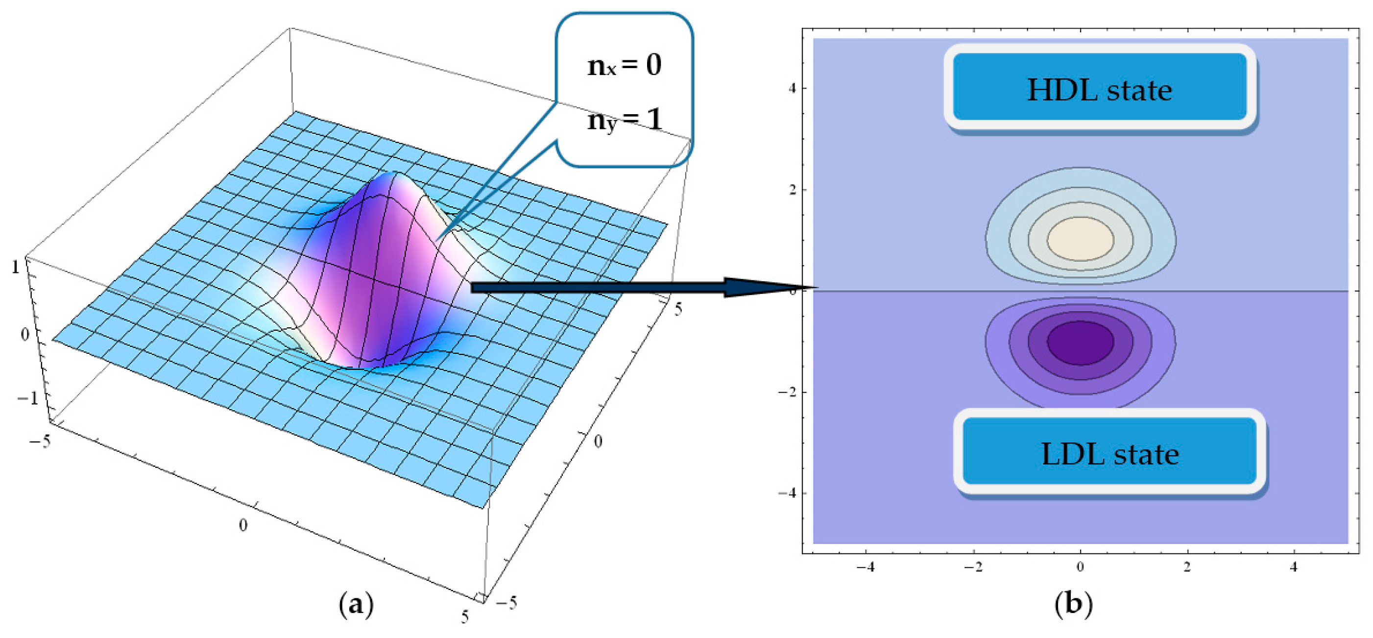
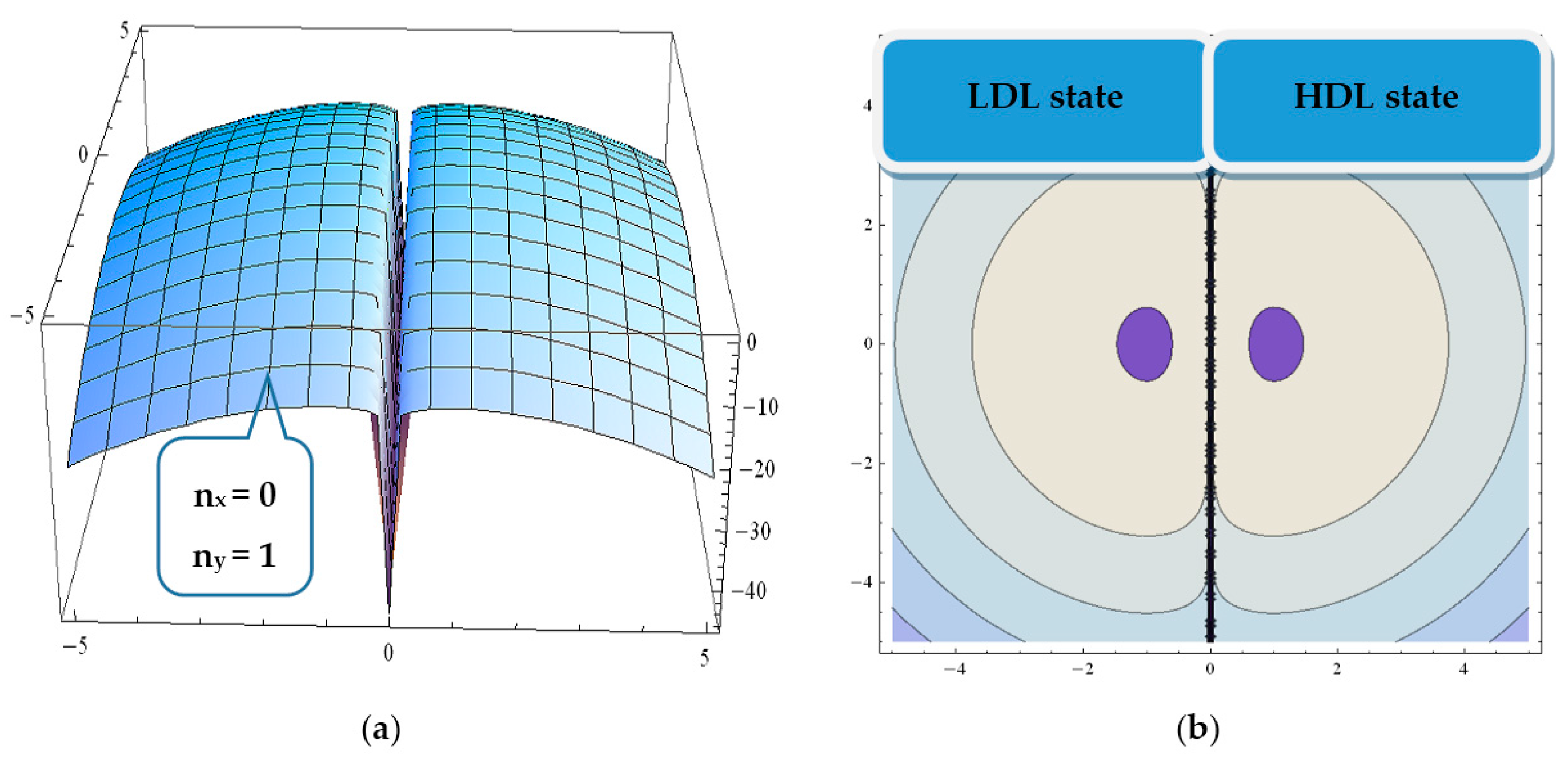
However, our fractal model extends the potential domain of applications for Schrödinger-type equations to every system in which the three conditions (an infinite or very large number of trajectories, a fractal dimension of individual trajectories, local irreversibility) are fulfilled. Macroscopic Schrödinger equations can be constructed, not based on Planck’s constant $\hslash$, but on constants that are specific to each biological structure and may emerge from their self-organization. Indeed, considering that both LDL and HDL are two different states of the same “entity”, i.e., cholesterol in the form of a LDL-HDL pair, the dynamics of such a biological structure can be described, for example, by means of a harmonic oscillator with a plane symmetry (states densities are described by means of associated Hermite polynomials, while the informational entropy is given by the logarithm of the same polynomials [6,7]); we note that these polynomials are solutions of Equation (9) for the stationary case and for plane symmetry. In this framework, in Figure 1 we present the states density $\rho =\Psi \overline{\Psi }$ for this system, where $\overline{\Psi }$ is the complex conjugate of $\Psi$ determined from Equation (9) for the stationary case, while in Figure 2 the associated informational entropy is shown. It can be seen that such a pair “operates” in a state of maximum informational entropy (for details see [12,15]).

5. Conclusions

In order to overcome the difficulties generated by the fact that the classical theories failed in explaining the dynamics of real complex sytems, i.e., fluid and kinetic models in the study of some phenomena, such as combustion, drug delivery, solid components separation in mixtures, and plasma ablation behavior, the fractal concepts and the corresponding non-differentiable theoretical models can be applied. Thus, the fractal entropy through non-differentiable Lie groups, compatible with a Hamiltonian-type formalism, was established. Furthermore, the pairs generating mechanism was explained through fractal entanglement states. We identified implications of the presented theory in the dynamics of some physical systems (the electron with a spin value of $+1/2$ is entangled with the electron with a spin value of $-1/2$, generating the Cooper pairs from superconductivity; the neutron and the proton are entangled, generating the pair from superfluidity) and biological structures (in the form of the “chameleon-like” behavior of cholesterol).