
A Study of the Transfer Entropy Networks on Industrial Electricity Consumption

1
School of Economics and Commerce, South China University of Technology, Guangzhou 510006, China
2
Industrial and Urban Development Research Center, South China University of Technology, Guangzhou 510006, China
3
School of Computer Science & Engineering, South China University of Technology, Guangzhou 510006, China
*
Author to whom correspondence should be addressed.
Entropy 2017, 19(4), 159; https://doi.org/10.3390/e19040159
Submission received: 11 January 2017
/
Revised: 29 March 2017
/
Accepted: 3 April 2017
/
Published: 13 April 2017
(This article belongs to the Special Issue Symbolic Entropy Analysis and Its Applications)
Abstract
:We study information transfer routes among cross-industry and cross-region electricity consumption data based on transfer entropy and the MST (Minimum Spanning Tree) model. First, we characterize the information transfer routes with transfer entropy matrixes, and find that the total entropy transfer of the relatively developed Guangdong Province is lower than others, with significant industrial cluster within the province. Furthermore, using a reshuffling method, we find that driven industries contain much more information flows than driving industries, and are more influential on the degree of order of regional industries. Finally, based on the Chu-Liu-Edmonds MST algorithm, we extract the minimum spanning trees of provincial industries. Individual MSTs show that the MSTs follow a chain-like formation in developed provinces and star-like structures in developing provinces. Additionally, all MSTs with the root of minimal information outflow industrial sector are of chain-form.
1. Introduction
Information flow is characterized by interaction, and is successfully used in analyzing economic systems [1,2,3]. A variety of methods can be used to extract the fundamental features caused by internal and external environments, such as cross-correlation [4], autocorrelation [5], and complexity [6,7]. However, although appropriate for measuring the relationships, they fail to illustrate the asymmetry and directionality among components of a system. The Granger causality method, proposed by Granger [8], has been used to measure the causality, but the information flow estimated by the traditional Granger causality method just provides binary information for causal relationships, whether one component is the Granger causality of the others or not. In other words, it is weak in measuring the strength of causality.
The main idea of exploring the interaction is the strength and direction of coupling. Transfer entropy (TE), developed by Schreiber [9], has a prominent contribution to detecting the mutual influence between the components of a dynamic system. It is worth mentioning that Granger causality and transfer entropy are equivalent for Gaussian distributions according to Barnett et al. [10]. After transfer entropy was proposed, it has been widely used in diverse fields, such as statistics [11,12], dynamical systems [13,14,15], social networks [16], physiology [17,18,19], the study of cellular automata in computer science [20,21], and so on.
On the basis of transfer entropy, some other transfer entropy analysis methods were also developed [22,23,24,25,26,27,28]. For instance, Marschinski and Kantz [29] introduced a measure called effective transfer entropy, by subtracting the effects of noise or of a highly volatile time series from the transfer entropy. This concept is now widely used, particularly in the study of the cerebral cortex.
In terms of the applications of transfer entropy to finance, Kwon and Yang [30] used the stock market indices of 25 countries and discovered that the biggest source of information flow is America, while most receivers are in the Asia-Pacific regions. By means of the minimum spanning tree, Standard and Poor’s 500 Index (S&P500) is a hub of information sources for the world stock markets. Kwon and Oh [31] found that the amount of information flows from an index to a stock is larger than the ones from a stock to an index between the stock market index and their component stocks. By using the stocks of the 197 largest companies in the world, Sandoval [32] assessed which companies influenced others according to sub-areas of the financial sector, and also analyzed the exchange of information between those stocks as seen by the transfer entropy and the network formed by them based on this measure. Making use of rolling estimations of extended matrixes and time-varying network topologies, Bekiros et al. [33] showed evidence of emphasized disparity of correlation and entropy-based centrality measurements for the U.S. equity and commodity futures markets between pre-crisis and post-crisis periods. M. Harré [34] used a novel variation of transfer entropy that dynamically adjusts to the arrival rate of individual prices and does not require the binning of data to show that quite different relationships emerge from those given by the conventional Pearson correlation.
Studying the industry section, Oh et al. [35] have investigated the information flows among 22 industry sectors in the Korean stock market by using the symbolic transfer entropy method. They found that the amount of information flows and the number of links during the financial crisis in the Korean stock market are higher than those before and after the market crisis. In the process of production, industries usually utilize raw materials and energy from other industries as inputs. Meanwhile, their outputs can also be consumed by other industries. Upstream industries supply raw materials for downstream industries; in return, downstream industries serve back upstream industries. Therefore, the industrial structure can be treated as a network, where each sector is represented by a node, and the intermediate products flow through the connections among the nodes.
Complex networks [36] and correlation-based algorithms like the MST model have been gradually adopted as efficient pattern-identification tools in complex systems, and are widely applied in financial markets. Trancoso et al. [37] researched interdependence and decoupling situations among emerging markets and developed countries in global economic networks, and demonstrated that emerging markets have not cohesively formed into global networks. However, they evolved into two main emerging market clusters of East European countries and East Asia. Zheng et al. [38] discussed the lag relationship between worldwide finance and commodities markets based on the MST evolution process. Zhang et al. [39] studied the world international shipping market, especially on evolutionary rules of MSTs, systemic risk, and the transmission relationship of Granger causality dynamics in pre-crisis and post-crisis times. Additionally, they replaced the Pearson distance of the traditional similarity index of sequences with Brownian distance, proposed by Székely and Rizzo [40], and better revealed the non-linear correlation among time series. Yao et al. [41] characterized the correlation evolution of South China industrial electricity consumption in pre-crisis and post-crisis periods, and demonstrated the industrial clustering from perspectives of industrial organization and specialization theories. Based on Granger causality networks, Yao et al. [42] also studied the industrial energy transferring routes among the industries of South China by distinguishing direct causality from the indirect, and with complementary graphs, ref. [42] proposed that industrial causal relationship can be heterogeneous, and provided insights for refining robust industrial causality frameworks.
Recently, most works of MST models studied multiple time series of price-based sequences, whereas a few studies focused on volume-based ones. These two types are significantly different: price-based sequences are mainly affected by cost and expectation, and are usually utilized for the analysis of prices of raw material and expectative behavioral determination; instead, volume-based ones directly reflect behaviors of economic units in the markets and they are consequently fitted for behavior analysis, such as consumption volume and investment volume. We choose monthly electricity consumption volume as an indicator of industrial production, based on the three reasons below: first, compared with industrial added value and GDP (Gross Domestic Product), the electricity consumption volume will be relatively less influenced by inflation, expectation factors, and will objectively reflect the behaviors of industrial production; second, the electricity consumption volume is the lead indicator for most economic variables’ future trend especially in China; third, the monthly electricity consumption volume is more stable in time, allowing us to record and study industrial correlation without delay.
Motivated by these previous studies, we mainly apply transfer entropy and MST models to analyzing industrial causality among the different industrial sectors. Based on the electricity consumption sequences, including the industries of five southern provinces in China, we construct transfer entropy networks to explore the information transfer routes among different industries.
The remaining arrangement of this article is as follows. Section 2 explains the definition of transfer entropy and the MST method. Section 3 describes the statistical characteristics of industrial electricity consumptions sequences. In Section 4 and Section 5, we demonstrate our detailed results and analysis of the empirical study. Finally, Section 6 is the conclusion of this paper.
2. Methodology Statement
2.1. Transfer Entropy
Given two discrete processes, Y and X, Shannon entropy [43], which measures the uncertainty of information, is represented as follows (Considering a discrete process Y):
The base 2 for the logarithm is chosen so that the measure is given in bits. The more bits that are needed to achieve optimal encoding of the process, the higher the uncertainty is.
According to the explanation of Maxwell’s Demon by Charles H. Bennett, the destruction of information is an irreversible process and hence it satisfies the second law of thermodynamics. Therefore, information has negative entropy. Since the generation of information is a process of involving negative entropy in a system, the sign of information entropy is opposite to the sign of thermodynamics entropy. Additionally, information entropy follows a law of decreasing.
On the basis of Shannon entropy, Kullback entropy is used to define the excess number of bits needed for encoding when improperly assuming a probability distribution of Y different things from . The formula is represented as follows [44]:
When it comes to the bivariate background, the mutual information of the two processes is given by reducing uncertainty compared to the circumstance where both processes are independent, i.e., where the joint distribution is given by the product of the marginal distributions, . The corresponding Kullback entropy, known as the formula for mutual information, is defined as follows [45,46]:
where the summation runs over the distinct values of x and y. Any form of statistical dependencies between different variables can be detected by mutual information. However, it is a symmetric measure and therefore any evidence related to the dynamics of information exchange is not available.
Transfer entropy is quantified by information flow, and measures the extent to which one dynamical process influences the transition probabilities of another process. It is applied for quantifying the strength and asymmetry of information flow between two components of a dynamical system. Learning from the experience mentioned above, we also define the transfer entropy relating k1 previous observations of process Y and k2 previous observations of process X as follows [47,48]:
where
Here, and represent the discrete states at time t of Y and X, respectively. and denote k1 and k2 dimensional delay vectors of the two time series of Y and X, respectively. The joint probability density function is the probability that the combination of , , and have particular values. The conditional probability density functions and determine the probability that has a particular value when the value of the previous samples and are known and are known, respectively. The reverse dependency is calculated by exchanging y and x of the joint and conditional probability density functions. The log is with base 2, thus the transfer entropy is given in bits.
The calculation of transfer entropy may involve significant computational burden, particularly when the number of variables is large. Therefore, simply assuming processes Y and X as Markov processes, we set k1 = k2 = 1. In fact, the parameter settings of k1 and k2 are not influential on the direction of information flow.
2.2. Symbolization
We estimate transfer entropy using a technique of symbolization, which has already been introduced with the concept of permutation entropy [49]. Staniek and Lehnertz [50] proposed a method for symbolization, and demonstrated numerically that symbolic transfer entropy is a robust and computationally efficient method for quantifying the dominant direction of information flow among time series from structurally identical and non-identical coupled systems.
The procedure of symbolization is demonstrated as follows:
Let and denote sequences of observations from discrete processes Y and X. Following ref. [50], we define the symbol by reordering the amplitude values of the time series and . Amplitude values are arranged in an ascending order , where m is the embedding dimension, and l denotes the time delay. In case of equal amplitude values, the rearrangement is carried out according to the associated index s, i.e., for , we write if . Therefore, every is uniquely mapped onto one of the m! possible permutations. A symbol is thus defined as , and with the relative frequency of symbols, we estimate the joint and conditional probabilities of the sequences of permutation indices. is also symbolized by this method. Finally, we estimate the transfer entropy using symbol sequences and on the basis of Formula (4).
The following is an example of symbolization. Assume that m = 3, l = 1, and there are 3! = 6 possible permutations. Let and . The amplitude values corresponds to a permutation or symbol , and the remainder can be processed by the same method. Then, and . We set the mapping relationships as: , , , , , . The symbol sequences are also denoted such that and . Therefore, continuous states can be also transformed into discrete states for the TE (Transfer Entropy) calculation.
If there is no extra explanation, we set m = 2, l = 1 for estimating transfer entropy in our study. This will be verified if it is a reasonable assumption.
Transfer entropy is explicitly asymmetric under the exchange of source and destination. It can thus provide information regarding the direction of interaction between two discrete processes. The asymmetric degree of information flow (ADIF) from X to Y can be defined as follows [51]:
If this value is positive, it means that the information flows run mostly from X to Y; whereas information flows in reverse run mostly from Y to X when the value is negative.
According to formula (8), we can obtain the net information outflow. Assuming that there are n discrete processes, we define the net asymmetric degree of information flow of X, which measures the net information outflow of X as follows:
2.3. Minimum Spanning Tree
Firstly, assuming N sectors, we construct a matrix to save the values of ADIF, and it is an anti-symmetric matrix.
Enlightened by the distance metric introduced by Onnela et al. [52], we define a pseudo-distance of MST by the procedure:
Here, is the pseudo-distance from i to j. c is an arbitrary constant, and the value of c is greater than the maximum value of . In our study, we set . Thus, we obtain a directed graph.
After the above process, we understand that: there is only one direction between two nodes for rejecting the other direction because of its negative value of ADIF; the greater the value of ADIF, the shorter the pseudo-distance of the two nodes.
Finally, illuminated by the intuition of taxonomy from the conventional minimum spanning tree, we step further with Chu–Liu–Edmonds MST algorithm [53,54] using the pseudo-distance above, and extract the directed minimum spanning tree from the transfer entropy networks, which may be interpreted with route and transmission recognition.
3. Data Description
The data we used are based on monthly industrial electricity consumption from January 2005 to December 2013 from five southern provinces in China, including GD (Guangdong Province), GX (Guangxi Zhuang Autonomous Region), YN (Yunnan Province), GZ (Guizhou Province) and HN (Hainan Province). Specifically, the power grids of these five provinces are operated by the China Southern Power Grid Limited Companies, which are relatively independent from the grids of the remaining 26 provinces operated by the State Grid Corporation of China, especially on power transmission and distribution. Thus, we sum the volume of industrial electricity consumption of these five provinces as the total electricity consumption volume of South China (NF). Consequently we obtain 6 observations units—GD, GX, YN, GZ, HN, and NF, covering 28 industries of manufacture of food, mining and dressing of ferrous metal ores, energy and chemical production, manufacture of machinery, etc.
Yao et al. [55] modeled industrial Granger networks using industrial electricity consumption as an indicator. This paper applied the same techniques. The reason, similar to Yao et al., is that: first, electricity consumption is a leading indicator of industrial production; and second, the monthly electricity consumption is timely, compared with a relative longer update period of industrial input–output tables of five years, and industrial GDP, with inflation by the office of statistics. Therefore, our study of the industrial causality mechanism based on industrial electricity consumption is less dependent on time.
In order to calculate TE, we convert industrial electricity consumption to the simple rate of change following the routine of ref. [35]:
where is the industrial electricity consumption in month t. Then, we calculate TE using the time series .
The codes and corresponding industries have been shown in Table 1. Table 2 demonstrates the statistical properties of the rate of change time series of the 28 South China industry sectors.
From Table 2, we have concluded that: the means range from 0.014 to 0.068; the sequence of V26 fluctuates the most, and the sequence of V15 has the least fluctuations; the kurtosis of V28 is the highest, and V15 has the lowest kurtosis; except for V15 and V27, the sequences of the remaining industries contain a degree of right skew; by means of calculating the JB-statistic (Jarque-Bera Statistic), we find that the sequences of V1, V4, and V15 follow Gaussian distributions.
4. Empirical Results on Transfer Entropy Networks
4.1. Industrial Analysis
Based on Formula (4), we calculate the transfer entropy of the rate of change on electricity consumption among different industrial sectors in five provinces of South China. As noted in Section 3, we list totally 140 exclusive industrial sectors of provinces (i.e., we issue different codes for same sectors from different provinces) ranking from 1 to 140 by industrial sectors of GD, GX, YN, GZ, and HN.
Figure 1 shows both the TEs of two sectors inside a given province and the cross-TEs of a given industrial sector between two provinces. A higher value of transfer entropy will be reflected by a brighter color in the heat map.
The square area surrounded by (0, 0), (28, 0), (0, 28), and (28, 28) contains many dark grids, reflecting the situation of the industrial correlation in GD. First, no matter the perspective of in-weight or out-weight, lower transfer entropy is observed in GD and there is no significant clustering for the remaining four provinces, implying relative independence of the internal information transfer structure of GD. Furthermore, other than lower transfer entropy inside the industrial sectors of GD, they show relatively high transfer entropy to industrial sectors of other provinces. This confirms a higher degree of order in industrial sectors of GD, but disorder for the influence of other provinces. The column dark lines in the figure illustrate that the corresponding industries received a lower entropy volume and have a higher degree of order.
Notes: Industrial sectors corresponding to the nine dark grid blocks in Figure 2 cover: Textile Industry (V8), Manufacture of Textile Garments, Fur, Feather, and Related Products (V9), Timber Processing, Products, and Manufacture of Furniture (V10), Papermaking and Paper Products (V11), Printing and Record Medium Reproduction (V12), Manufacture of Cultural, Educational, Sports, and Entertainment Articles (V13), Manufacture of Medicines (V16), Manufacture of Chemical Fibers (V17), Rubber and Plastic Products (V18), Nonmetal Mineral Products (V19), Metal Products (V22), Manufacture of General-purpose and Special-purpose Machinery (V23), Manufacture of Transport, Electrical, and Electronic Machinery (V24).
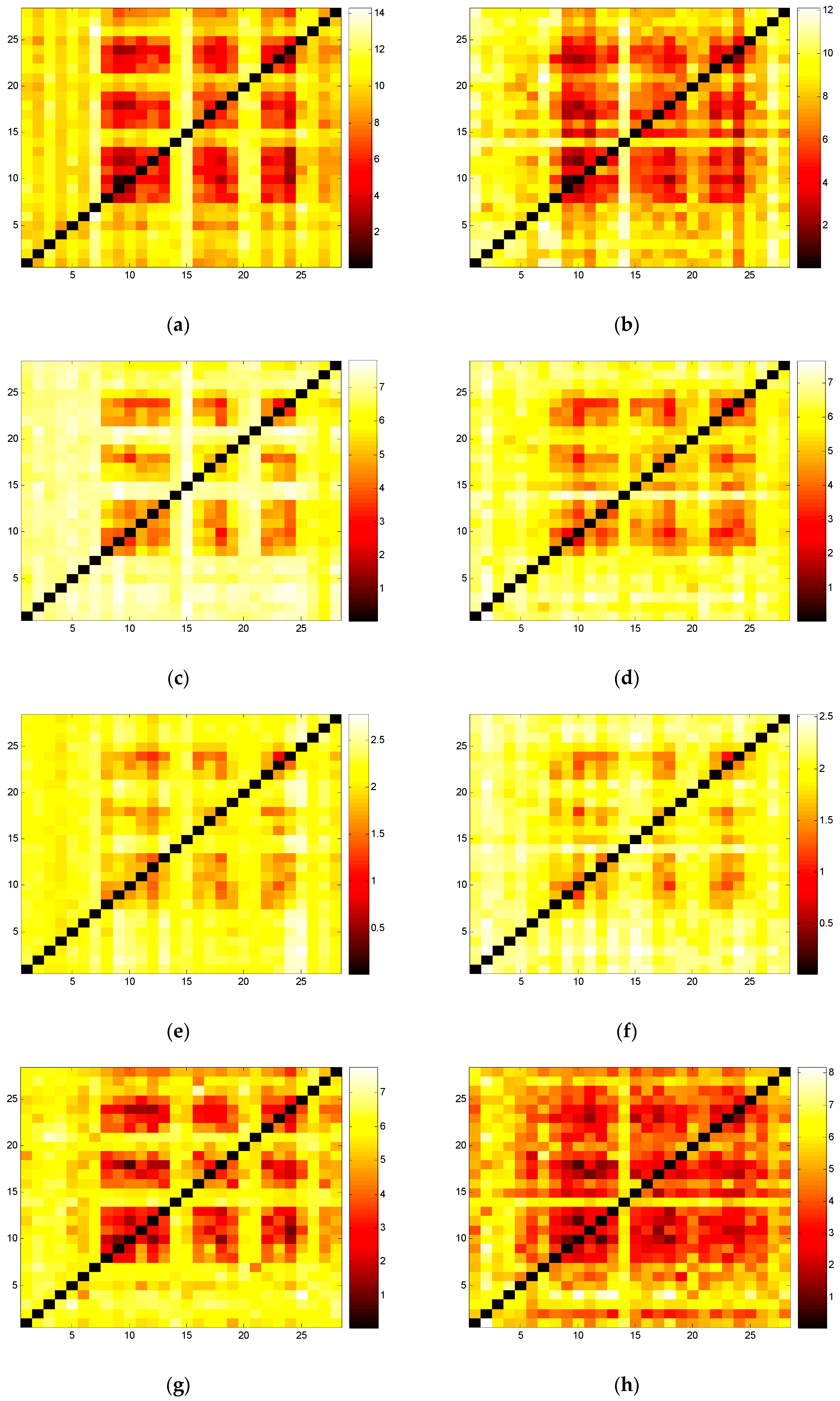
By summing the electricity consumption of a given industry of the five provinces of GD, GX, YN, GZ, and HN, we gain the total electricity consumption of the 28 industries of South China. Figure 2a is the transfer entropy heat map of South China. Nine grid blocks with lower transfer entropy imply that ordered industrial sectors tend to cluster and each grid block is one industrial cluster. Blocks close to the diagonal stand for those with a low transfer entropy and a high degree of order among the internal industrial sectors. Blocks far from the diagonal stand for clusters with higher transfer entropy and a high degree of order for other external clusters. Thus, transfer entropy can be used for a measure of the degree of order of an industrial cluster. Comparing Figure 2a,b, we find high similarity between them: 13 industrial sectors in dark grid blocks are of a higher degree of order. We also find that the industrial clusters of NF are more significant than the industrial clusters of GD. The reason is likely that NF consists of GD, GX, YN, GZ, and HN, thus there is a complementary effect among the five provinces in the industrial division.
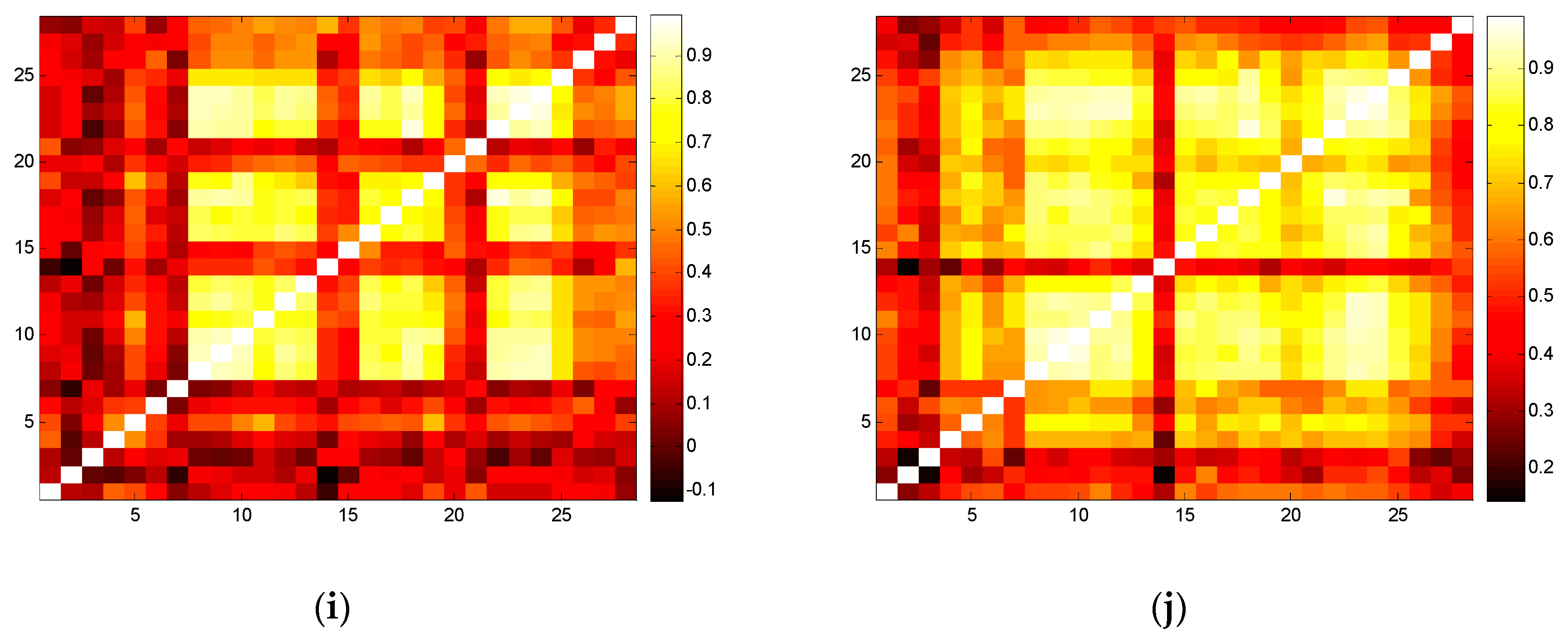
Comparing transfer entropy with the correlation coefficient, we conclude that lower transfer entropy always corresponds to a higher correlation coefficient. Figure 2a–h show that the different parameter settings of m and l have significantly different TE, but it is not influential on the correlation of industrial sectors, and the general features of the heat maps with the different parameter settings are similar. Therefore, the parameter setting of m = 2, l = 1 is a better choice for relieving the computational burden.
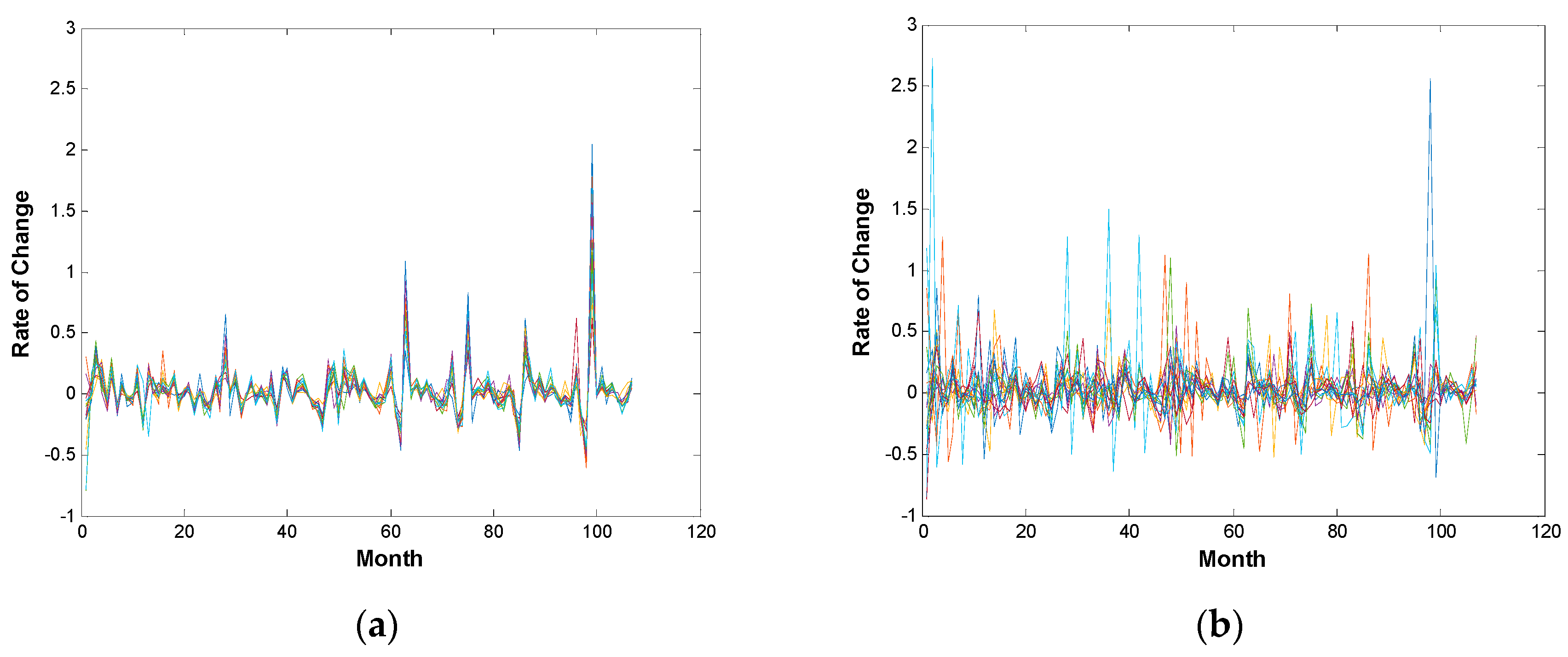
According to the information extracted from the nine dark grid blocks, we plot the line chart of the rate of change time series. Different color lines correspond to different industrial sectors. We find that the industrial sectors in Figure 3a have a higher degree of uniformity on the fluctuation of the rate of change, while the ones in Figure 3b do not show synchronization features. Hence, the transfer entropy is able to interpret the homogeneity of the industrial sectors to some extent, and it has shown that lower entropy volume always corresponds to a higher degree of order.
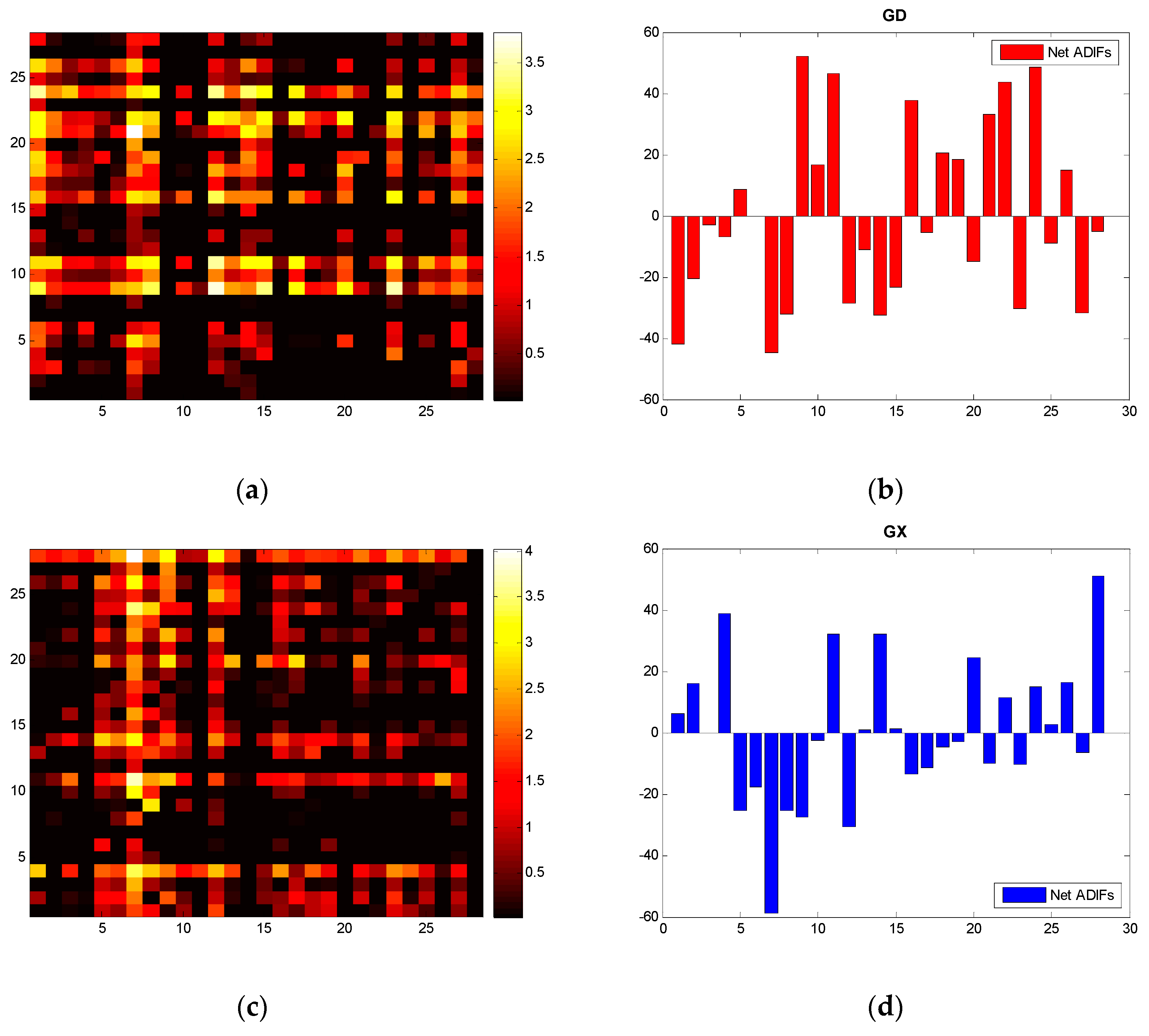
For the information flow among the industries of each province, and referring to Formulas (7) and (8), we compute the ADIF of five provinces in South China, and present the heat maps and histograms in Figure 4.
Notes: according to the formula in Section 2, the ADIF matrix is anti-symmetric. We set 0 for a negative ADIF on the heat maps for a more clear explanation.
With the heat maps and histograms, we find even distributions of bright spots of GD, but it appears to have uneven distributions of YN. Referring to the histogram of YN, we see the net information outflow of V9 and V26 is much higher than the others. This also confirms the balanced development and industrial specialization of GD and the seriously imbalanced development and probable homogeneous information of YN.
It is worth mentioning that Comprehensive Utilization of Waste (V26) will be greatly affected if the production of other industrial sectors increases. Other than HN, the remaining four provinces exhibit significant net information outflow, especially in YN and GZ. Our finding demonstrates that the increase (decrease) of electricity consumption of V26 will lead to the increase (decrease) of electricity consumption of other industries and similarly verifies this process of information feedback: V26 as a measure of waste reproduction implies the upgrade of green economies in South China.
4.2. Reshuffled Analysis
With the industrial electricity consumption of the whole of South China, we study the in-weight and out-weight of transfer entropy and compute the reshuffling transfer entropy by the three methods below [56]:
Here, for all i, is a shuffled time series of X, and is a shuffled time series of Y. Assuming that the data size is n, there are n! possibilities to shuffle the time series. Hence we set M = 1000 intermediately. These three methods randomly shuffle the state of each time point, but the expectation, standard deviation, and distribution before and after the shuffling remain approximately the same.
From Figure 5, we conclude that Figure 5f preserves the most features in Figure 5e. This implies that the target sequence Y contains much information, since the general distribution of in-weight does not change by shuffling X, but by keeping X unchanged. Besides, only shuffling Y (Figure 5c,g) and simultaneously shuffling X and Y (Figure 5d,h) achieve similar effects. By comparing TE with the shuffled data based on the three methods, we demonstrate that the inflows and outflows of transfer entropy from real data are not obtained by chance. Therefore, the characteristics of target sequences can approximately determine the values of the transfer entropy. The industries representing for target sequences tend to be driven industries, other than driving industries. Driven industries usually contain much more information flows and are more influential on determining the order of degree distribution of the whole industrial system.
5. Route Extraction of the Causality Structure and Dynamics
Effective models of transfer entropy networks provide the basic framework for extracting the causality structure and dynamics of the rate of change on electricity consumption among industrial sectors. Considering the characteristics of weighted directed networks, we extract the most probable route of directed transfer entropy networks of different provinces, which is composed of the links of the lowest weight based on the Chu-Liu-Edmonds MST algorithm and provide related decision support of macroeconomic adjustment for economic systems.
The basic processes of the algorithm covers three steps: (1) Judge whether all nodes of the original graphs are attainable with a fixed root; if there is not any available option, no MST can be extracted from this graph; (2) Traverse all the edges for the least in-edge of the nodes except the root node, accumulate the weights, and form a new graph with the least weights; (3) Judge whether any loop exists in that graph, if not, that graph is the MST we acquire; otherwise, shrink that directed loop into a node and go back to Step (2).
5.1. Analysis of a Single Province
Traditional stimulus policies for developing industries are sometimes groundless in choosing target industries. According to the leading industry theory and strategic emerging industry theory, the ignorance of the intrinsic topology of causality probably leads to serious industrial overcapacity. Therefore, with the causality structures among industries, policymakers tend to determine a more precise regulation strategy on industrial systems by pointing out those key nodes, especially the root nodes of industries, and reduce the potential overcapacity problems caused by overall stimulus [55].
Based on different root-chosen methods, we extract the MSTs of Figure 6 and Figure 7 from the ADIF transfer entropy network of each province. Figure 6 is rooted in the industry of maximal information outflows [30] while Figure 7 is rooted in the industry of minimal information outflows. We can obviously observe that the hierarchical structure of information flows along the arrows.
Figure 6 shows the information spreading routes of a given root. The MSTs of GD and GX follow a significant hierarchical structure, implying the routes and effects of influence from the roots are heterogeneous, and the influence on some nodes is indirect. The MSTs of other provinces are star-like, and hence the influence from the roots is homogeneous. From the perspectives of industrial correlation, the correlation of GD and GX will be higher than the remaining three provinces and therefore tend to balance development.
Based on Figure 6 and Figure 7, we find the diameter of Figure 7 is usually greater than the one of Figure 6, and the MSTs rooted in the industry of minimal information outflow are usually of chain-like form and with feedback loops. The structure of minimal information outflow can characterize the maximal order of the system and can be used as a reference of the system evolutionary direction.
Combining the industrial need to regulate with the topology of causality, policymakers may precisely stimulate industries by choosing root nodes, hub nodes, and probably reduce serious overcapacity problems of other industries.
5.2. Inter-Provincial Analysis
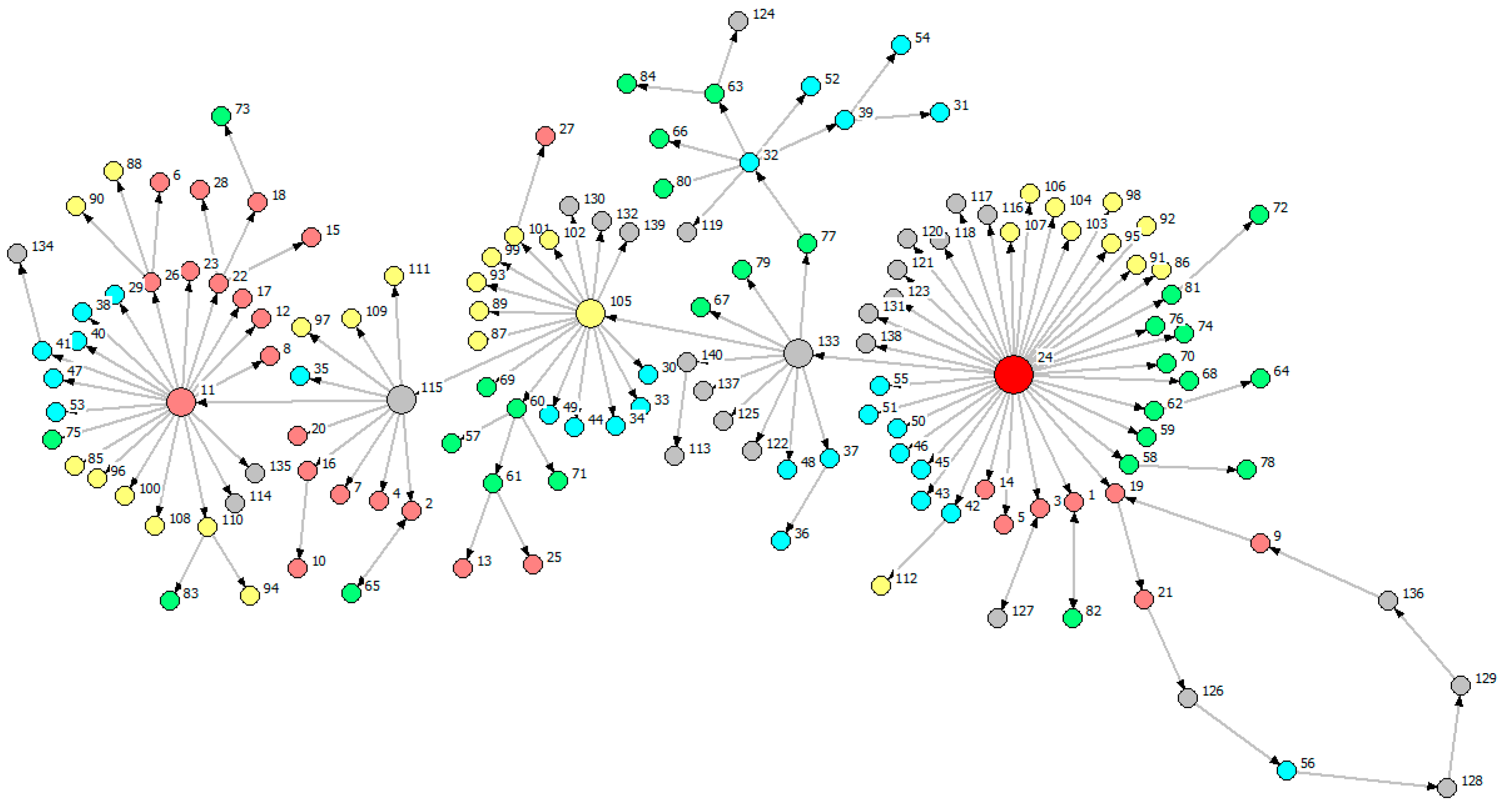
Including the 140 provincial industries of the five provinces of South China, we study their cross-province interactive relationship. Rooted on a node of GD, Figure 8 is rooted in the industry of maximal information outflow while Figure 9 is rooted in the industry of minimal information outflow.
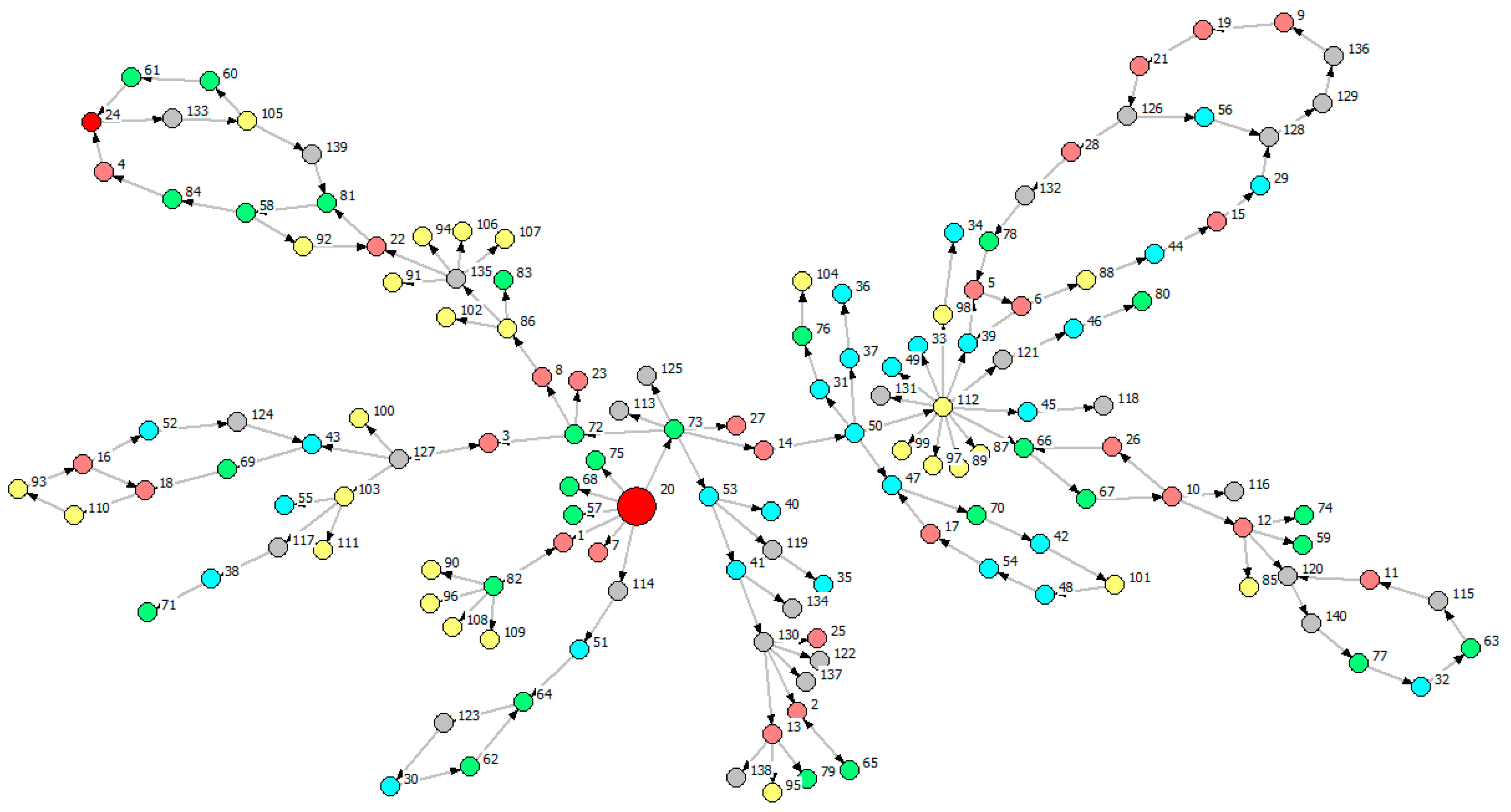
Comparing the MST of Figure 8 with the MST of Figure 9, we find a star-like structure in Figure 8 and a chain-like structure in Figure 9. According to the information in Table 3, we found 12 feedback loops inside the chain-like structure in Figure 9, and some of the loops are nested. We also observe that the node with maximal information outflow is surrounded by more nodes than the node with minimal information outflow. It demonstrates that the root node in Figure 8 plays a greater role than the one in Figure 9. The reason why the two MSTs are different from each other is probably because the more information the root node has, the more efficient the network is in the method of information transfer.
Notes: Colors of Nodes: GD (red), GX (blue), YN (green), GZ (yellow), HN (grey).
We introduce Figure 8 by three parts: the node group linked with the root node V24; the hierarchical structure that information flows spread along according to the determined route V133 V105 V115 V11 (four key nodes are HN Smelting and Pressing of Nonferrous Metals (V133), GZ Smelting and Pressing of Nonferrous Metals (V105), HN Mining and Dressing of Ferrous Metal Ores (V115), GD Papermaking and Paper Products (V11)); feedback loop V19 V21 V126 V56 V128 V129 V136 V9 V19. We notice that most of the red nodes are directly or indirectly linked with V115 and V11 which are far away from the root node, and many of grey nodes, labeling industries of HN, are close to the root node.
6. Conclusions
Based on the transfer entropy matrixes of each provincial industry, we found a lower transfer entropy of the relatively developed GD, and higher transfer entropy for the remaining four provinces. According to the principle of entropy increase, we proposed that GD exhibits a higher degree of internal industrial order, but the remaining provinces tends to be more disordered, and hence, transfer entropy can be a measure of the degree of industry order.
Besides the other provinces, GD shows significant block-clustering of internal transfer entropy, implying its independence of the internal industrial information transfer structure. In this aspect, the~transfer entropy can be used as a measure of the industrial clustering emergence. By reshuffling, we found the target industries or driven industries tend to contain much more information flows than driving industries, and are more influential on determining the degree of regional industrial order.
Finally, based on the Chu-Liu-Edmonds MST algorithm, we studied their provincial MSTs. Individual MSTs show chain-like structures in developed provinces and star-like structures in developing areas. Rooted in the minimal information outflow sectors, the generated MSTs all follow a chain-like structure, which are similar to the cross-province results. Therefore, the chain-like structure and feedback loop can be used as a measure of industrial ordered evolution.
Acknowledgments
This research was supported by the National Natural Science Foundation of China (Grant 71201060), Research Fund for the Doctoral Program of Higher Education (Grant 20120172120051), and the Fundamental Research Funds for the Central Universities (Grant 2015ZZ059, 2015ZDXM04).
Author Contributions
Canzhong Yao and Pengcheng Kuang conceived and designed the experiments; Qingwen Lin contributed analysis tools. Boyi Sun contributed the discussion and revision.
Conflicts of Interest
The authors declare no conflict of interest.
References
- Miśkiewicz, J.; Ausloos, M. Influence of Information Flow in the Formation of Economic Cycles. Underst. Complex. Syst. 2006, 9, 223–238. [Google Scholar]
- Zhang, Q.; Liu, Z. Coordination of Supply Chain Systems: From the Perspective of Information Flow. In Proceedings of the 4th International Conference on Wireless Communications, Networking and Mobile Computing, Dalian, China, 12–14 October 2008; pp. 1–4. [Google Scholar]
- Eom, C.; Kwon, O.; Jung, W.S.; Kim, S. The effect of a market factor on information flow between stocks using the minimal spanning tree. Phys. A Stat. Mech. Appl. 2009, 389, 1643–1652. [Google Scholar] [CrossRef]
- Shi, W.; Shang, P. Cross-sample entropy statistic as a measure of synchronism and cross-correlation of stock markets. Nonlinear Dyn. 2012, 71, 539–554. [Google Scholar] [CrossRef]
- Gao, F.J.; Guo, Z.X.; Wei, X.G. The Spatial Autocorrelation Analysis on the Regional Divergence of Economic Growth in Guangdong Province. Geomat. World 2010, 4, 29–34. [Google Scholar]
- Mantegna, R.N.; Stanley, H.E. An Introduction to Econophysics: Correlations and Complexity in Finance; Cambridge University Press: Cambridge, UK, 1999. [Google Scholar]
- Song, H.L.; Zhang, Y.; Li, C.L.; Wang, C.P. Analysis and evaluation of structural complexity of circular economy system’s industrial chain. J. Coal Sci. Eng. 2013, 19, 427–432. [Google Scholar] [CrossRef]
- Granger, C.W.J. Investigating causal relations by econometric models and cross-spectral methods. Econometrica 1969, 37, 424–438. [Google Scholar] [CrossRef]
- Schreiber, T. Measuring Information Transfer. Phys. Rev. Lett. 2000, 85, 461–464. [Google Scholar] [CrossRef] [PubMed]
- Barnett, L.; Barrett, A.B.; Seth, A.K. Granger Causality and Transfer Entropy Are Equivalent for Gaussian Variables. Phys. Rev. Lett. 2009, 103, 4652–4657. [Google Scholar] [CrossRef] [PubMed]
- Amblard, P.O.; Michel, O.J.J. The Relation between Granger Causality and Directed Information Theory: A Review. Entropy 2012, 15, 113–143. [Google Scholar] [CrossRef]
- Liu, L.; Hu, H.; Deng, Y.; Ding, N.D. An Entropy Measure of Non-Stationary Processes. Entropy 2014, 16, 1493–1500. [Google Scholar] [CrossRef]
- Liang, X.S. The Liang-Kleeman Information Flow: Theory and Applications. Entropy 2013, 1, 327–360. [Google Scholar] [CrossRef]
- Prokopenko, M.; Lizier, J.T.; Price, D.C. On Thermodynamic Interpretation of Transfer Entropy. Entropy 2013, 15, 524–543. [Google Scholar] [CrossRef]
- Materassi, M.; Consolini, G.; Smith, N.; de Marco, R. Information Theory Analysis of Cascading Process in a Synthetic Model of Fluid Turbulence. Entropy 2014, 16, 1272–1286. [Google Scholar] [CrossRef]
- Steeg, G.V.; Galstyan, A. Information transfer in social media. In Proceedings of the 21st International Conference on World Wide Web, Lyon, France, 16–20 April 2012. [Google Scholar]
- Vicente, R.; Wibral, M.; Lindner, M.; Pipa, G. Transfer entropy—A model-free measure of effective connectivity for the neurosciences. J. Comput. Neurosci. 2011, 30, 45–67. [Google Scholar] [CrossRef] [PubMed]
- Shew, W.L.; Yang, H.; Yu, S.; Roy, R. Information Capacity and Transmission are Maximized in Balanced Cortical Networks with Neuronal Avalanches. J. Neurosci. 2011, 31, 55–63. [Google Scholar] [CrossRef] [PubMed]
- Faes, L.; Nollo, G.; Porta, A. Compensated Transfer Entropy as a Tool for Reliably Estimating Information Transfer in Physiological Time Series. Entropy 2013, 15, 198–219. [Google Scholar]
- Lizier, J.T.; Prokopenko, M.; Zomaya, A.Y. Local information transfer as a spatiotemporal filter for complex systems. Phys. Rev. E 2008, 77, 026110. [Google Scholar] [CrossRef] [PubMed]
- Lizier, J.T.; Mahoney, J.R. Moving Frames of Reference, Relativity and Invariance in Transfer Entropy and Information Dynamics. Entropy 2013, 15, 177–197. [Google Scholar] [CrossRef]
- Lizier, J.T.; Heinzle, J.; Horstmann, A.; Haynes, J.D. Multivariate information-theoretic measures reveal directed information structure and task relevant changes in fMRI connectivity. J. Comput. Neurosci. 2011, 30, 85–107. [Google Scholar] [CrossRef] [PubMed]
- Lam, L.; Mcbride, J.W.; Swingler, J. Renyi’s information transfer between financial time series. Phys. A Stat. Mech. Appl. 2011, 391, 2971–2989. [Google Scholar]
- Runge, J.; Heitzig, J.; Petoukhov, V.; Kurths, J. Escaping the curse of dimensionality in estimating multivariate transfer entropy. Phys. Rev. Lett. 2012, 108, 1–5. [Google Scholar] [CrossRef] [PubMed]
- Dimpfl, T.; Peter, F.J. The impact of the financial crisis on transatlantic information flows: An intraday analysis. J. Int. Financ. Mark. Inst. Money 2014, 31, 1–13. [Google Scholar] [CrossRef]
- Melzer, A.; Schella, A. Symbolic transfer entropy analysis of the dust interaction in the presence of wakefields in dusty plasmas. Phys. Rev. E 2014, 89, 187–190. [Google Scholar] [CrossRef] [PubMed]
- Lobier, M.; Siebenhühner, F.; Palva, S.; Palva, J.M. Phase transfer entropy: A novel phase-based measure for directed connectivity in networks coupled by oscillatory interactions. Neuroimage 2014, 85, 853–872. [Google Scholar] [CrossRef] [PubMed]
- Daugherty, M.S.; Jithendranathan, T. A study of linkages between frontier markets and the U.S. equity markets using multivariate GARCH and transfer entropy. J. Multinatl. Financ. Manag. 2015, 32, 95–115. [Google Scholar] [CrossRef]
- Marschinski, R.; Kantz, H. Analysing the information flow between financial time series. Eur. Phys. J. B 2002, 30, 275–281. [Google Scholar] [CrossRef]
- Kwon, O.; Yang, J.S. Information flow between stock indices. Europhys. Lett. 2008, 82, 68003. [Google Scholar] [CrossRef]
- Kwon, O.; Oh, G. Asymmetric information flow between market index and individual stocks in several stock markets. Europhys. Lett. 2012, 97, 28007–28012. [Google Scholar] [CrossRef]
- Sandoval, L. Structure of a Global Network of Financial Companies Based on Transfer Entropy. Entropy 2014, 16, 110–116. [Google Scholar] [CrossRef]
- Bekiros, S.; Nguyen, D.K.; Junior, L.S.; Uddin, G.S. Information diffusion, cluster formation and entropy-based network dynamics in equity and commodity markets. Eur. J. Oper. Res. 2017, 256, 945–961. [Google Scholar] [CrossRef]
- Harré, M. Entropy and Transfer Entropy: The Dow Jones and the Build Up to the 1997 Asian Crisis. In Proceedings of the International Conference on Social Modeling and Simulation, plus Econophysics Colloquium 2014; Springer: Zurich, Switzerland, 2015. [Google Scholar]
- Oh, G.; Oh, T.; Kim, H.; Kwon, O. An information flow among industry sectors in the Korean stock market. J. Korean Phys. Soc. 2014, 65, 2140–2146. [Google Scholar] [CrossRef]
- Yang, Y.; Yang, H. Complex network-based time series analysis. Phys. A Stat. Mech. Appl. 2008, 387, 1381–1386. [Google Scholar] [CrossRef]
- Trancoso, T. Emerging markets in the global economic network: Real(ly) decoupling? Phys. A Stat. Mech. Appl. 2014, 395, 499–510. [Google Scholar] [CrossRef]
- Zheng, Z.; Yamasaki, K.; Tenenbaum, J.N.; Stanley, H.E. Carbon-dioxide emissions trading and hierarchical structure in worldwide finance and commodities markets. Phys. Rev. E 2012, 87, 417–433. [Google Scholar] [CrossRef] [PubMed]
- Zhang, X.; Podobnik, B.; Kenett, D.Y.; Stanley, H.E. Systemic risk and causality dynamics of the world international shipping market. Phys. A Stat. Mech. Appl. 2014, 415, 43–53. [Google Scholar] [CrossRef]
- Székely, G.J.; Rizzo, M.L. Rejoinder: Brownian distance covariance. Ann. Appl. Stat. 2010, 3, 1303–1308. [Google Scholar] [CrossRef]
- Yao, C.Z.; Lin, J.N.; Liu, X.F. A study of hierarchical structure on South China industrial electricity-consumption correlation. Phys. A Stat. Mech. Appl. 2016, 444, 129–145. [Google Scholar] [CrossRef]
- Yao, C.Z.; Lin, Q.W.; Lin, J.N. A study of industrial electricity consumption based on partial Granger causality network. Phys. A Stat. Mech. Appl. 2016, 461, 629–646. [Google Scholar] [CrossRef]
- Shannon, C.E. A Mathematical Theory of Communication. Bell Syst. Tech. J. 1948, 27, 379–423, 623–656. [Google Scholar] [CrossRef]
- Olivares, S.; Paris, M.G.A. Quantum estimation via the minimum Kullback entropy principle. Phys. Rev. A 2007, 76, 538. [Google Scholar] [CrossRef]
- Dimpfl, T.; Peter, F.J. Using Transfer Entropy to Measure Information Flows Between Financial Markets. Stud. Nonlinear Dyn. Econom. 2013, 17, 85–102. [Google Scholar] [CrossRef]
- Teng, Y.; Shang, P. Transfer entropy coefficient: Quantifying level of information flow between financial time series. Phys. A Stat. Mech. Appl. 2016, 469, 60–70. [Google Scholar] [CrossRef]
- Nichols, J.M.; Seaver, M.; Trickey, S.T.; Todd, M.D.; Olson, C. Detecting nonlinearity in structural systems using the transfer entropy. Phys. Rev. E Stat. Nonlinear Soft Matter Phys. 2005, 72, 046217. [Google Scholar] [CrossRef] [PubMed]
- Boba, P.; Bollmann, D.; Schoepe, D.; Wester, N. Efficient computation and statistical assessment of transfer entropy. Front. Phys. 2015, 3, 267–278. [Google Scholar] [CrossRef]
- Bandt, C.; Pompe, B. Permutation entropy: A natural complexity measure for time series. Phys. Rev. Lett. 2002, 88, 174102. [Google Scholar] [CrossRef] [PubMed]
- Staniek, M.; Lehnertz, K. Symbolic transfer entropy. Phys. Rev. Lett. 2008, 100, 3136–3140. [Google Scholar] [CrossRef] [PubMed]
- Chen, G.; Xie, L.; Chu, J. Measuring causality by taking the directional symbolic mutual information approach. Chin. Phys. B 2013, 22, 556–560. [Google Scholar] [CrossRef]
- Onnela, J.P.; Chakraborti, A.; Kaski, K.; Kertesz, J. Dynamic Asset Trees and Black Monday. Phys. A Stat. Mech. Appl. 2002, 324, 247–252. [Google Scholar] [CrossRef]
- Chu, Y.J.; Liu, T.H. On the Shortest Arborescence of a Directed Graph. Sci. Sin. 1965, 14, 1396–1400. [Google Scholar]
- Edmonds, J. Optimum branchings. J. Res. Natl. Bur. Stand. B 1967, 71, 233–240. [Google Scholar] [CrossRef]
- Yao, C.Z.; Lin, J.N.; Lin, Q.W.; Zheng, X.Z.; Liu, X.F. A study of causality structure and dynamics in industrial electricity consumption based on Granger network. Phys. A Stat. Mech. Appl. 2016, 462, 297–320. [Google Scholar] [CrossRef]
- Sensoy, A.; Sobaci, C.; Sensoy, S.; Alali, F. Effective transfer entropy approach to information flow between exchange rates and stock markets. Chaos Solitons Fractals 2014, 68, 180–185. [Google Scholar] [CrossRef]
Figure 1.
Transfer entropy heat map among industrial sectors of five provinces in South China where m = 2 and l = 1. (Code in the Y-axis denotes industry of information outflow, and code in the X-axis denotes industry of information inflow; GD: 1–28, GX: 29–56, YN: 57–84, GZ: 85–112, HN: 113–140).
Figure 1.
Transfer entropy heat map among industrial sectors of five provinces in South China where m = 2 and l = 1. (Code in the Y-axis denotes industry of information outflow, and code in the X-axis denotes industry of information inflow; GD: 1–28, GX: 29–56, YN: 57–84, GZ: 85–112, HN: 113–140).
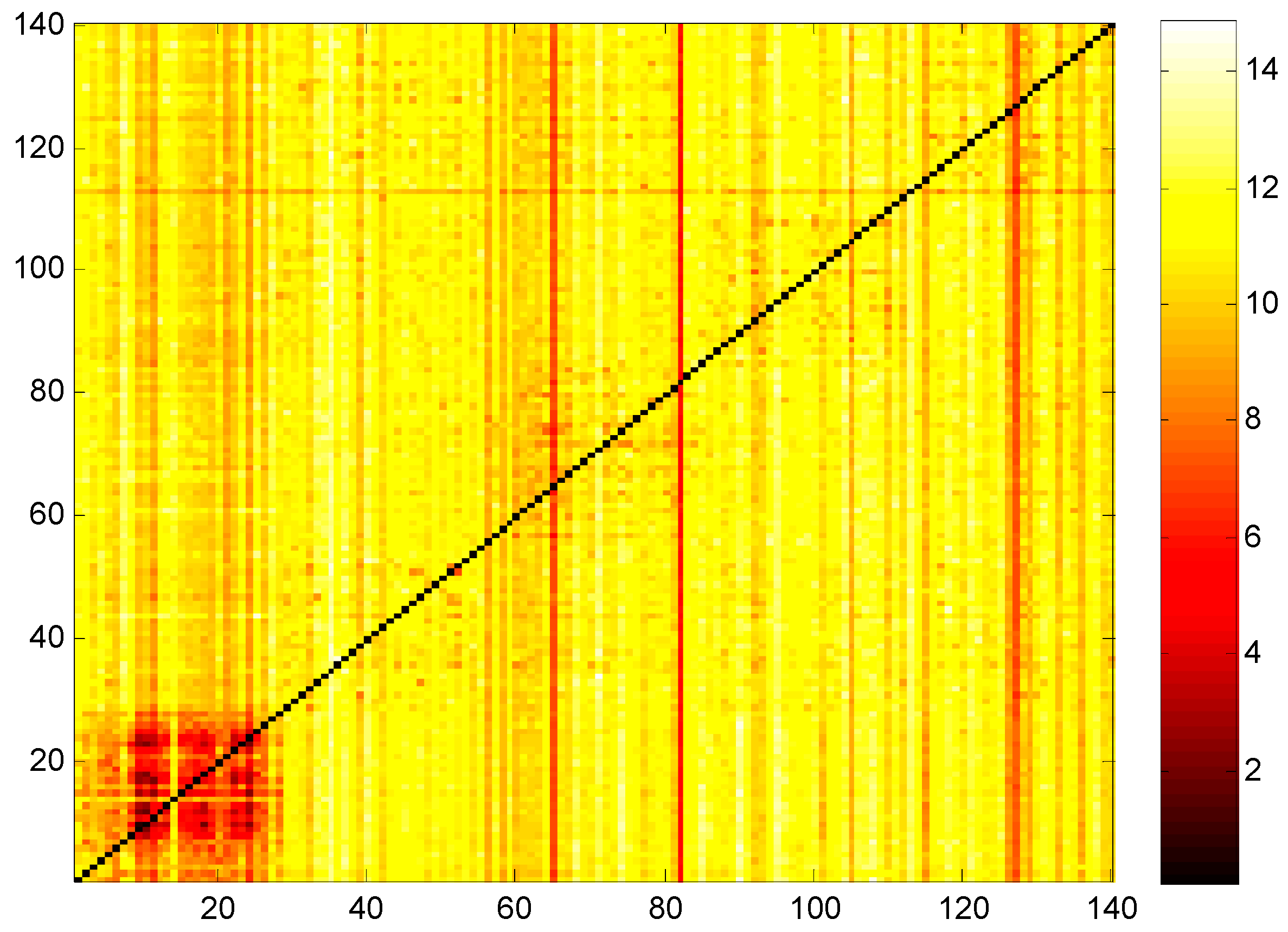
Figure 2.
(a) Transfer entropy heat map of South China where m = 2 and l = 1; (b) Transfer entropy heat map of GD where m = 2 and l = 1; (c) Transfer entropy heat map of South China where m = 3 and l = 1; (d) Transfer entropy heat map of GD where m = 3 and l = 1; (e) Transfer entropy heat map of South China where m = 4 and l = 1; (f) Transfer entropy heat map of GD where m = 4 and l = 1; (g) Transfer entropy heat map of South China where m = 2 and l = 2; (h) Transfer entropy heat map of GD where m = 2 and l = 2; (i) Spearman’s rank correlation coefficient heat map of South China; (j) Spearman’s rank correlation coefficient heat map of GD.


Figure 3.
Line chart of the rate of change time series: (a) contains 13 industrial sectors corresponding to nine dark grid blocks in Figure 2; (b) contains the remaining 15 industrial sectors.
Figure 3.
Line chart of the rate of change time series: (a) contains 13 industrial sectors corresponding to nine dark grid blocks in Figure 2; (b) contains the remaining 15 industrial sectors.

Figure 4.
Heat maps of the five provinces based on ADIF (Asymmetric Degree of Information Flow): (a) GD; (c) GX; (e) YN; (g) GZ; (i) HN; Net ADIF histograms: (b) GD; (d) GX; (f) YN; (h) GZ; (j) HN.
Figure 4.
Heat maps of the five provinces based on ADIF (Asymmetric Degree of Information Flow): (a) GD; (c) GX; (e) YN; (g) GZ; (i) HN; Net ADIF histograms: (b) GD; (d) GX; (f) YN; (h) GZ; (j) HN.

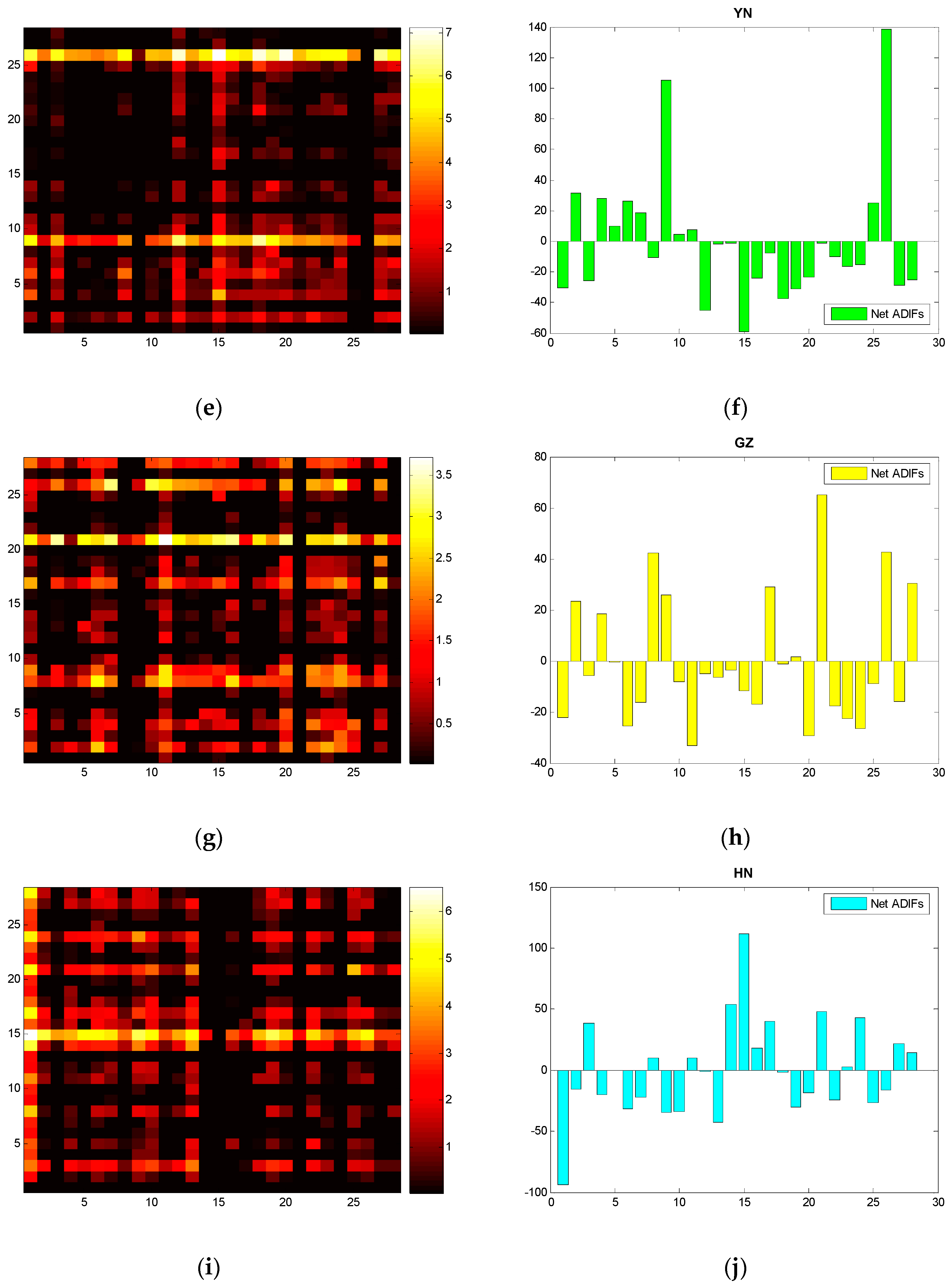
Figure 5.
Transfer entropy of South China: (a) initial out-weight boxplot; (b) out-weight boxplot after shuffling X; (c) out-weight boxplot after shuffling Y; (d) out-weight boxplot after shuffling both X and Y; (e) initial in-weight boxplot; (f) in-weight boxplot after shuffling X; (g) in-weight boxplot after shuffling Y; (h) in-weight boxplot after shuffling both X and Y.
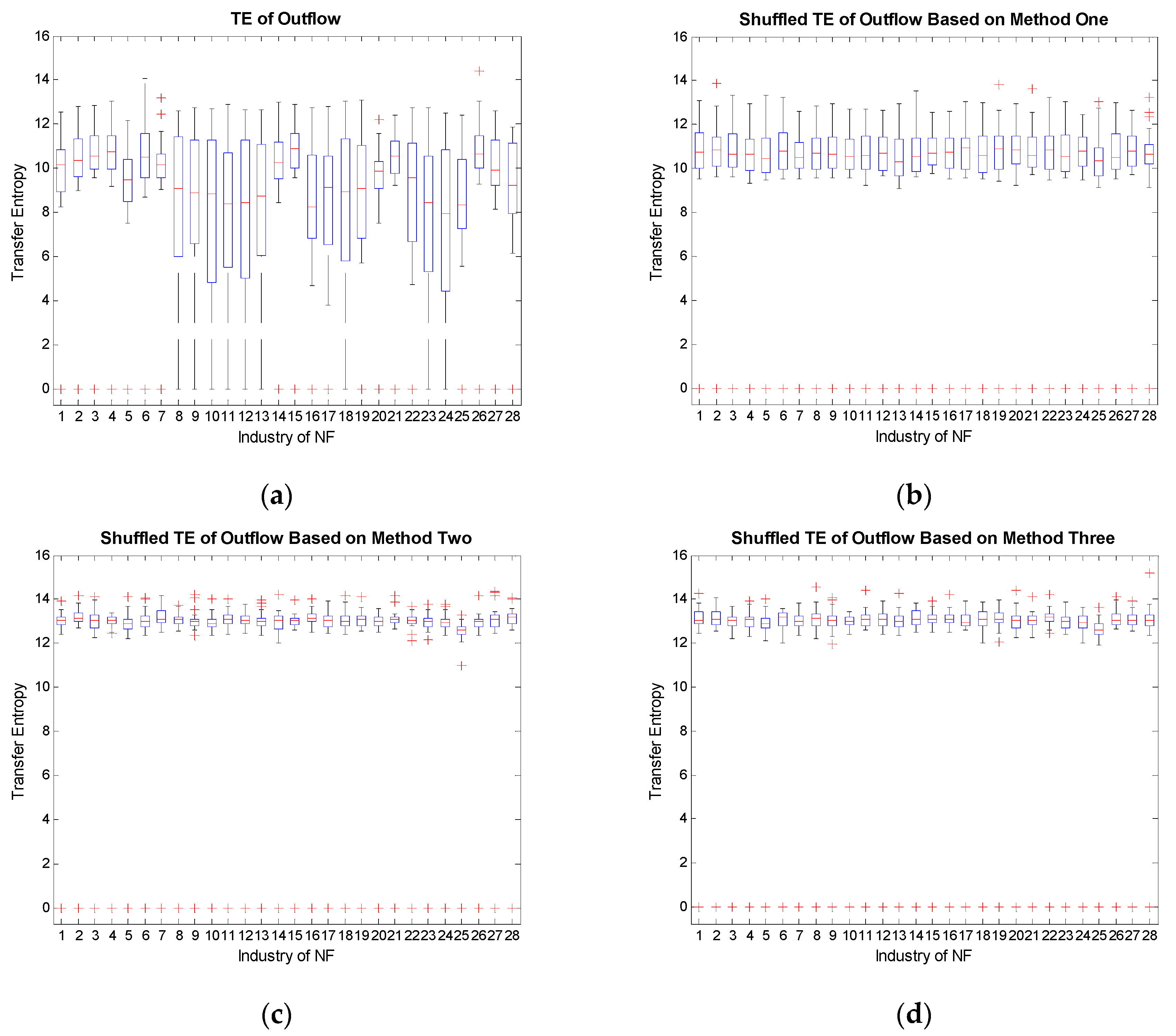
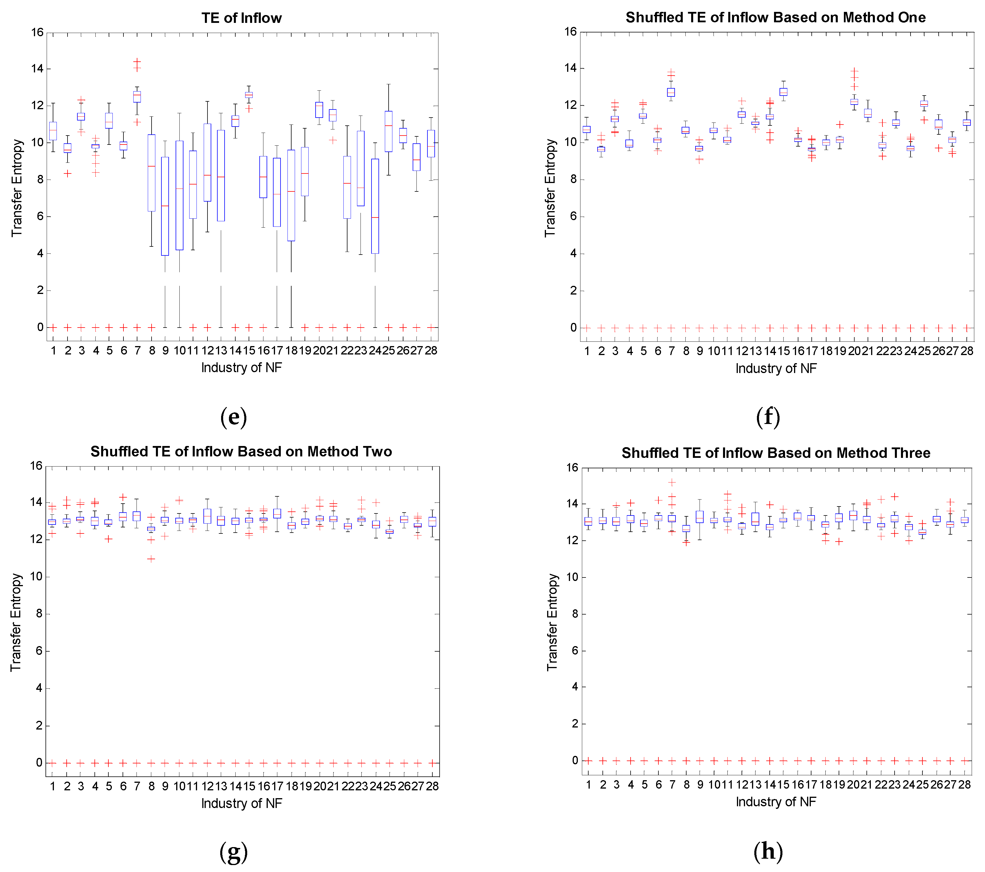
Figure 6.
Provincial MSTs (Minimum Spanning Trees) rooted in the industry of maximal information outflow: (a) GD (root: V9); (b) GX (root: V28); (c) YN (root: V26); (d) GZ (root: V21); (e) HN (root: V15).
Figure 6.
Provincial MSTs (Minimum Spanning Trees) rooted in the industry of maximal information outflow: (a) GD (root: V9); (b) GX (root: V28); (c) YN (root: V26); (d) GZ (root: V21); (e) HN (root: V15).
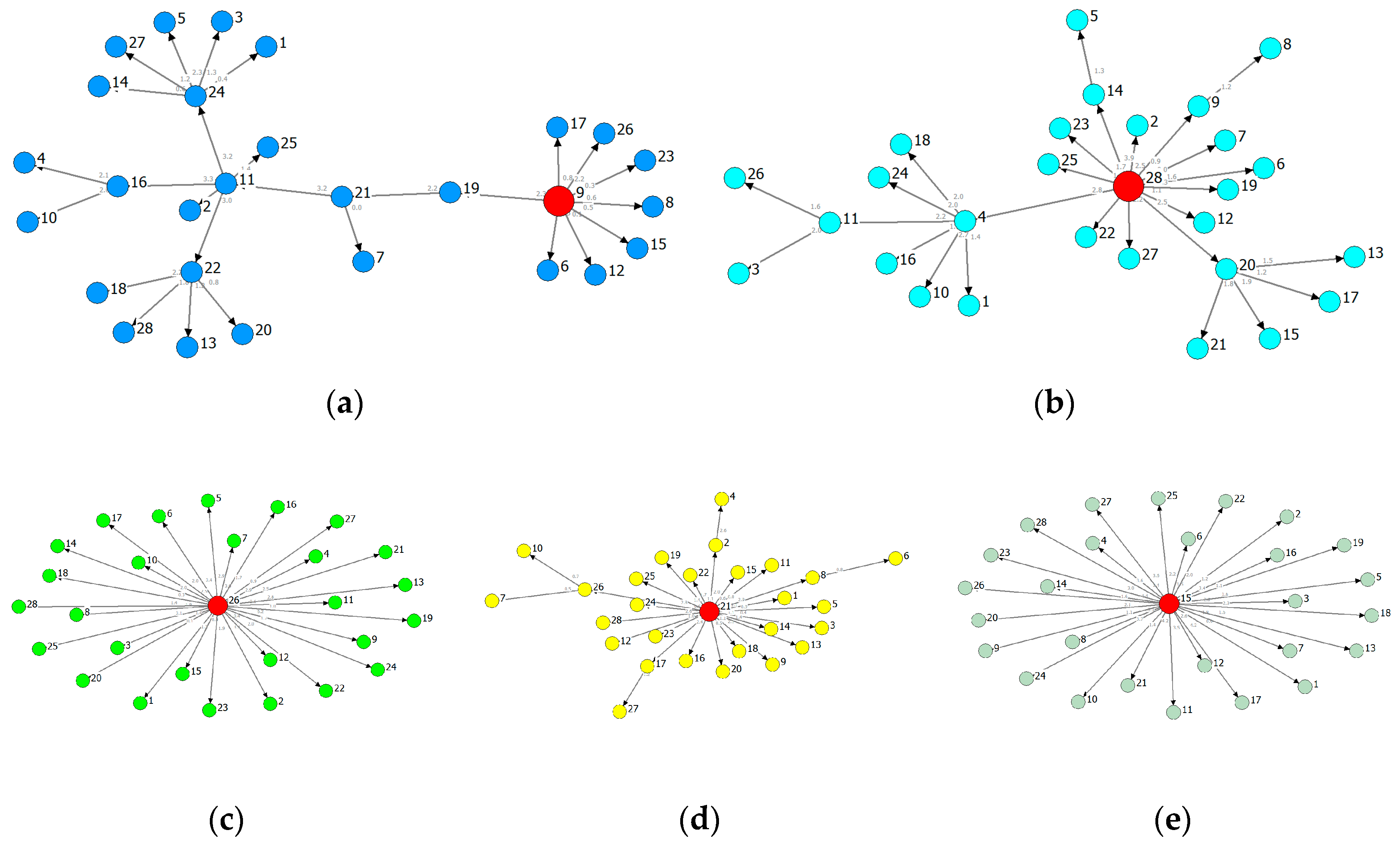
Figure 7.
Provincial MSTs rooted in the industry of minimal information outflow: (a) GD (root: V5); (b) GX (root: V13); (c) YN (root: V10); (d) GZ (root: V19); (e) HN (root: V23).
Figure 7.
Provincial MSTs rooted in the industry of minimal information outflow: (a) GD (root: V5); (b) GX (root: V13); (c) YN (root: V10); (d) GZ (root: V19); (e) HN (root: V23).
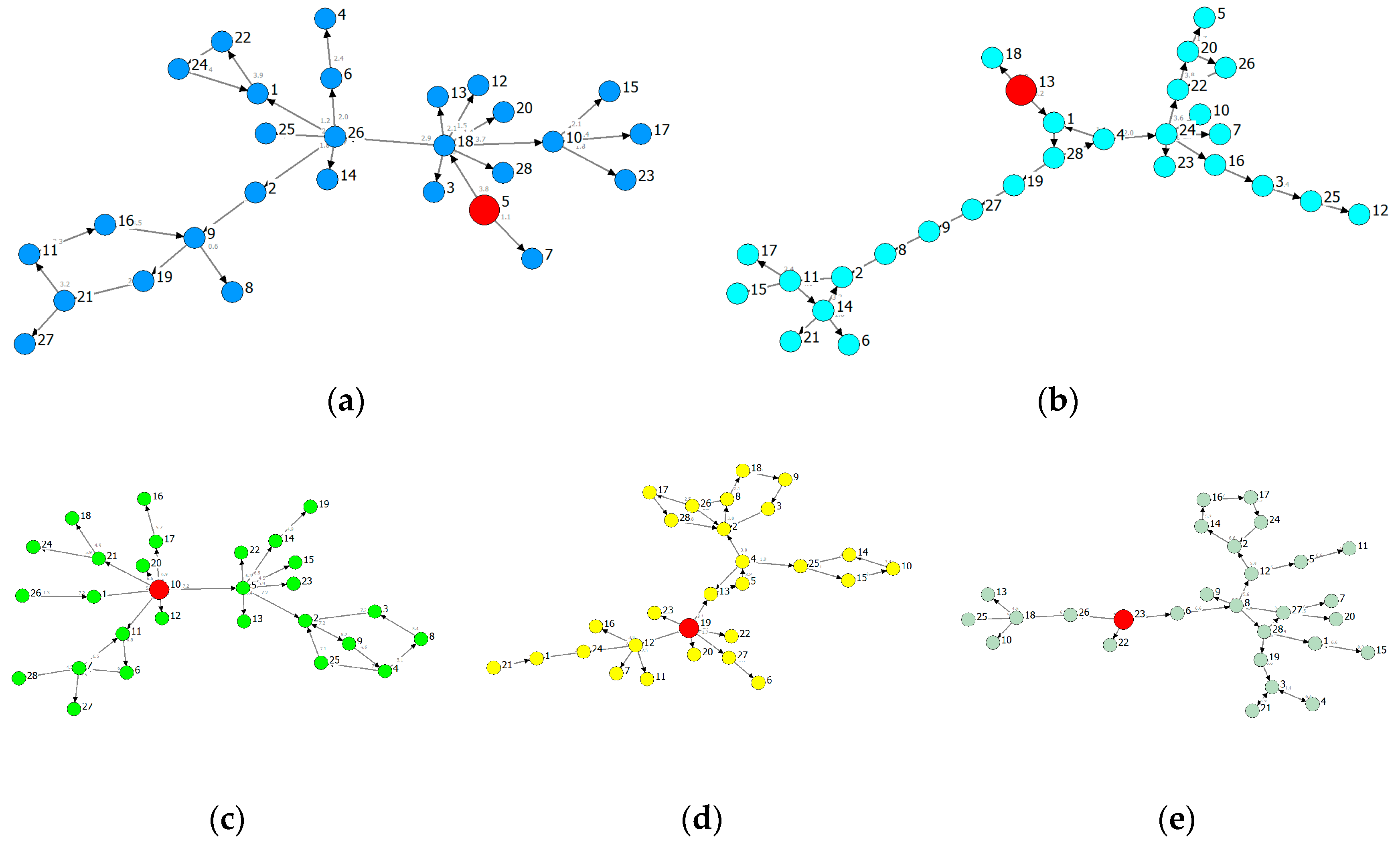
Figure 8.
Cross-province MST of South China (Rooted in the industry of maximal information outflow of GD, i.e., GD Manufacture of Transport, Electrical and Electronic Machinery (V24)).
Figure 8.
Cross-province MST of South China (Rooted in the industry of maximal information outflow of GD, i.e., GD Manufacture of Transport, Electrical and Electronic Machinery (V24)).

Figure 9.
Cross-province MST of South China (Rooted in the industry of minimal information outflow of GD, i.e., GD Smelting and Pressing of Ferrous Metals (V20)).
Figure 9.
Cross-province MST of South China (Rooted in the industry of minimal information outflow of GD, i.e., GD Smelting and Pressing of Ferrous Metals (V20)).


Table 1.
Code of the nodes and corresponding industries.
| Code | Industry |
|---|---|
| V1 | Mining and Washing of Coal |
| V2 | Extraction of Petroleum and Natural Gas |
| V3 | Mining and Dressing of Ferrous Metal Ores |
| V4 | Mining and Dressing of Nonferrous Metal Ores |
| V5 | Mining and Dressing of Nonmetal Ores |
| V6 | Mining and Dressing of Other Ores |
| V7 | Manufacture of Food, Beverage, and Tobacco |
| V8 | Textile Industry |
| V9 | Manufacture of Textile Garments, Fur, Feather, and Related Products |
| V10 | Timber Processing, Products, and Manufacture of Furniture |
| V11 | Papermaking and Paper Products |
| V12 | Printing and Record Medium Reproduction |
| V13 | Manufacture of Cultural, Educational, Sports, and Entertainment Articles |
| V14 | Petroleum Refining, Coking, and Nuclear Fuel Processing |
| V15 | Manufacture of Raw Chemical Materials and Chemical Products |
| V16 | Manufacture of Medicines |
| V17 | Manufacture of Chemical Fibers |
| V18 | Rubber and Plastic Products |
| V19 | Nonmetal Mineral Products |
| V20 | Smelting and Pressing of Ferrous Metals |
| V21 | Smelting and Pressing of Nonferrous Metals |
| V22 | Metal Products |
| V23 | Manufacture of General-purpose and Special-purpose Machinery |
| V24 | Manufacture of Transport, Electrical, and Electronic Machinery |
| V25 | Other Manufactures |
| V26 | Comprehensive Utilization of Waste |
| V27 | Production and Supply of Gas |
| V28 | Production and Supply of Water |
Table 2.
Statistical properties of the rate of change time series of 28 South China industry sectors.
Table 2.
Statistical properties of the rate of change time series of 28 South China industry sectors.
| Code | Mean | STD | Skewness | Kurtosis | JB-Statistic | Probability |
|---|---|---|---|---|---|---|
| V1 | 0.028593 | 0.159676 | 0.022191 | 3.728845 | 2.377116 | 0.304660 |
| V2 | 0.050715 | 0.325692 | 1.383137 | 6.100709 | 76.98059 | 0.000000 |
| V3 | 0.030155 | 0.194552 | 0.753318 | 6.280401 | 58.09648 | 0.000000 |
| V4 | 0.022994 | 0.141241 | 0.113567 | 3.899567 | 3.837782 | 0.146770 |
| V5 | 0.02181 | 0.186587 | 1.930843 | 14.32913 | 638.7092 | 0.000000 |
| V6 | 0.068385 | 0.321179 | 1.665988 | 8.443783 | 181.6184 | 0.000000 |
| V7 | 0.014926 | 0.159499 | 0.827264 | 5.225815 | 34.29224 | 0.000000 |
| V8 | 0.031674 | 0.284571 | 3.837147 | 26.56859 | 2739.081 | 0.000000 |
| V9 | 0.033462 | 0.257691 | 3.051374 | 21.80968 | 1743.420 | 0.000000 |
| V10 | 0.025657 | 0.209002 | 2.190527 | 14.91872 | 718.9044 | 0.000000 |
| V11 | 0.014068 | 0.131022 | 1.103867 | 6.753926 | 84.55699 | 0.000000 |
| V12 | 0.021448 | 0.222096 | 1.316007 | 12.19274 | 407.6430 | 0.000000 |
| V13 | 0.02337 | 0.246749 | 2.609256 | 21.83432 | 1702.926 | 0.000000 |
| V14 | 0.024322 | 0.172692 | 1.40529 | 11.33782 | 345.1580 | 0.000000 |
| V15 | 0.017798 | 0.116727 | −0.23907 | 3.183362 | 1.169192 | 0.557331 |
| V16 | 0.022083 | 0.135479 | 1.56146 | 8.714324 | 189.0606 | 0.000000 |
| V17 | 0.016444 | 0.193304 | 2.335657 | 13.33235 | 573.2465 | 0.000000 |
| V18 | 0.032043 | 0.236534 | 2.773104 | 18.81172 | 1251.771 | 0.000000 |
| V19 | 0.022901 | 0.160858 | 1.515492 | 9.312477 | 218.6109 | 0.000000 |
| V20 | 0.020431 | 0.135593 | 0.646182 | 4.847269 | 22.65996 | 0.000012 |
| V21 | 0.017874 | 0.121844 | 0.397835 | 6.999253 | 74.12922 | 0.000000 |
| V22 | 0.036121 | 0.24267 | 2.783564 | 18.11194 | 1156.329 | 0.000000 |
| V23 | 0.024369 | 0.177941 | 2.167856 | 15.36133 | 765.0540 | 0.000000 |
| V24 | 0.025961 | 0.180863 | 1.461672 | 9.638931 | 234.6035 | 0.000000 |
| V25 | 0.032045 | 0.233692 | 0.967952 | 5.123345 | 36.80940 | 0.000000 |
| V26 | 0.043833 | 0.367526 | 4.013498 | 29.4557 | 3407.669 | 0.000000 |
| V27 | 0.020359 | 0.180185 | −0.43386 | 8.581308 | 142.2384 | 0.000000 |
| V28 | 0.02955 | 0.286529 | 6.398114 | 58.17704 | 14303.45 | 0.000000 |
Table 3.
The information of the above MSTs.
| Root | Key Nodes | Number of Feedback Loop | |
|---|---|---|---|
| Figure 8 | V24 | Radial nodes of hierarchical structure (V133, V105, V115, V11) | 1 |
| Figure 9 | V20 | Nodes with an out-degree more than 3 (V12, V13, V50, V53, V72,V73, V82,V86, V103, V112, V127, V130,V135) | 12 |
Notes: The feedback loop doesn’t contain two-node loop in our study.
© 2017 by the authors. Licensee MDPI, Basel, Switzerland. This article is an open access article distributed under the terms and conditions of the Creative Commons Attribution (CC BY) license (http://creativecommons.org/licenses/by/4.0/).
Share and Cite
MDPI and ACS Style
Yao, C.-Z.; Kuang, P.-C.; Lin, Q.-W.; Sun, B.-Y. A Study of the Transfer Entropy Networks on Industrial Electricity Consumption. Entropy 2017, 19, 159. https://doi.org/10.3390/e19040159
AMA Style
Yao C-Z, Kuang P-C, Lin Q-W, Sun B-Y. A Study of the Transfer Entropy Networks on Industrial Electricity Consumption. Entropy. 2017; 19(4):159. https://doi.org/10.3390/e19040159
Chicago/Turabian StyleYao, Can-Zhong, Peng-Cheng Kuang, Qing-Wen Lin, and Bo-Yi Sun. 2017. "A Study of the Transfer Entropy Networks on Industrial Electricity Consumption" Entropy 19, no. 4: 159. https://doi.org/10.3390/e19040159
Note that from the first issue of 2016, this journal uses article numbers instead of page numbers. See further details here.