Modelling Urban Sprawl Using Remotely Sensed Data: A Case Study of Chennai City, Tamilnadu


 ,
,  ,
, 
Abstract
:1. Introduction
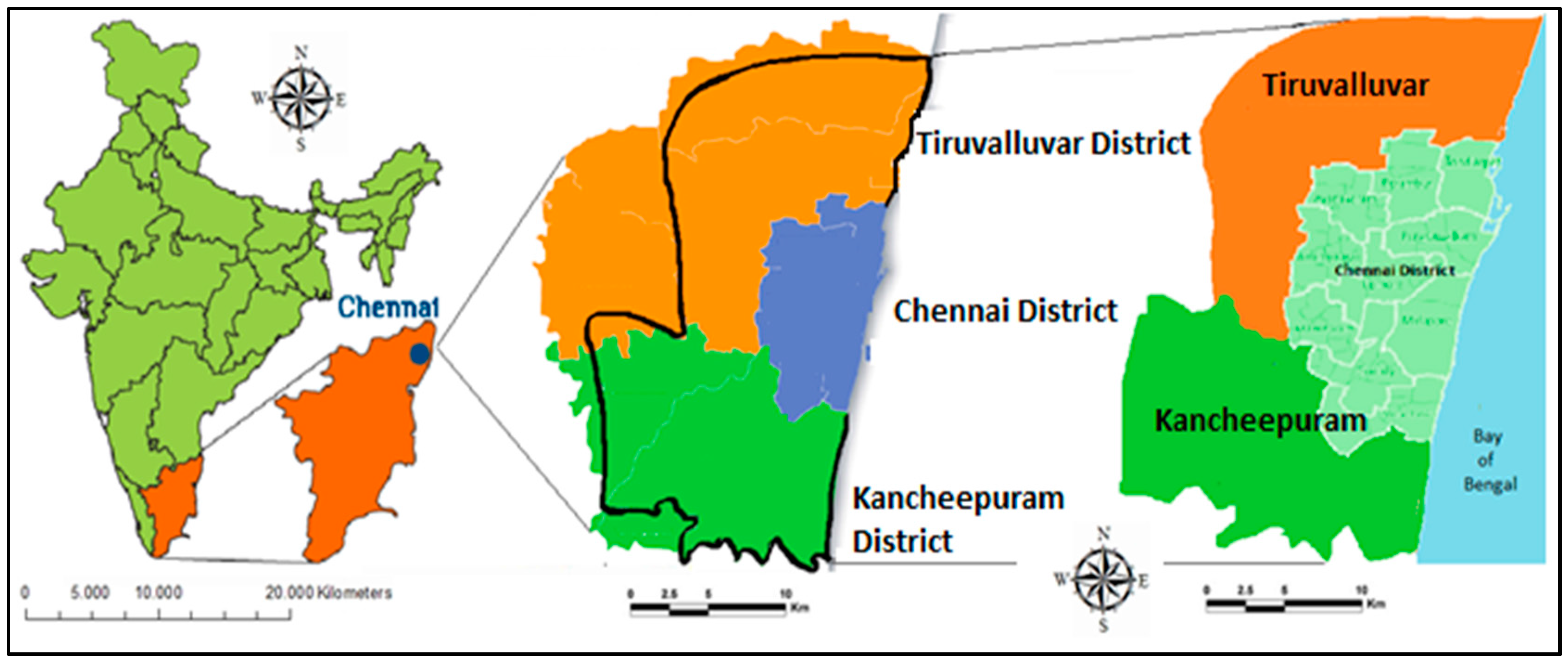
2. Study Area
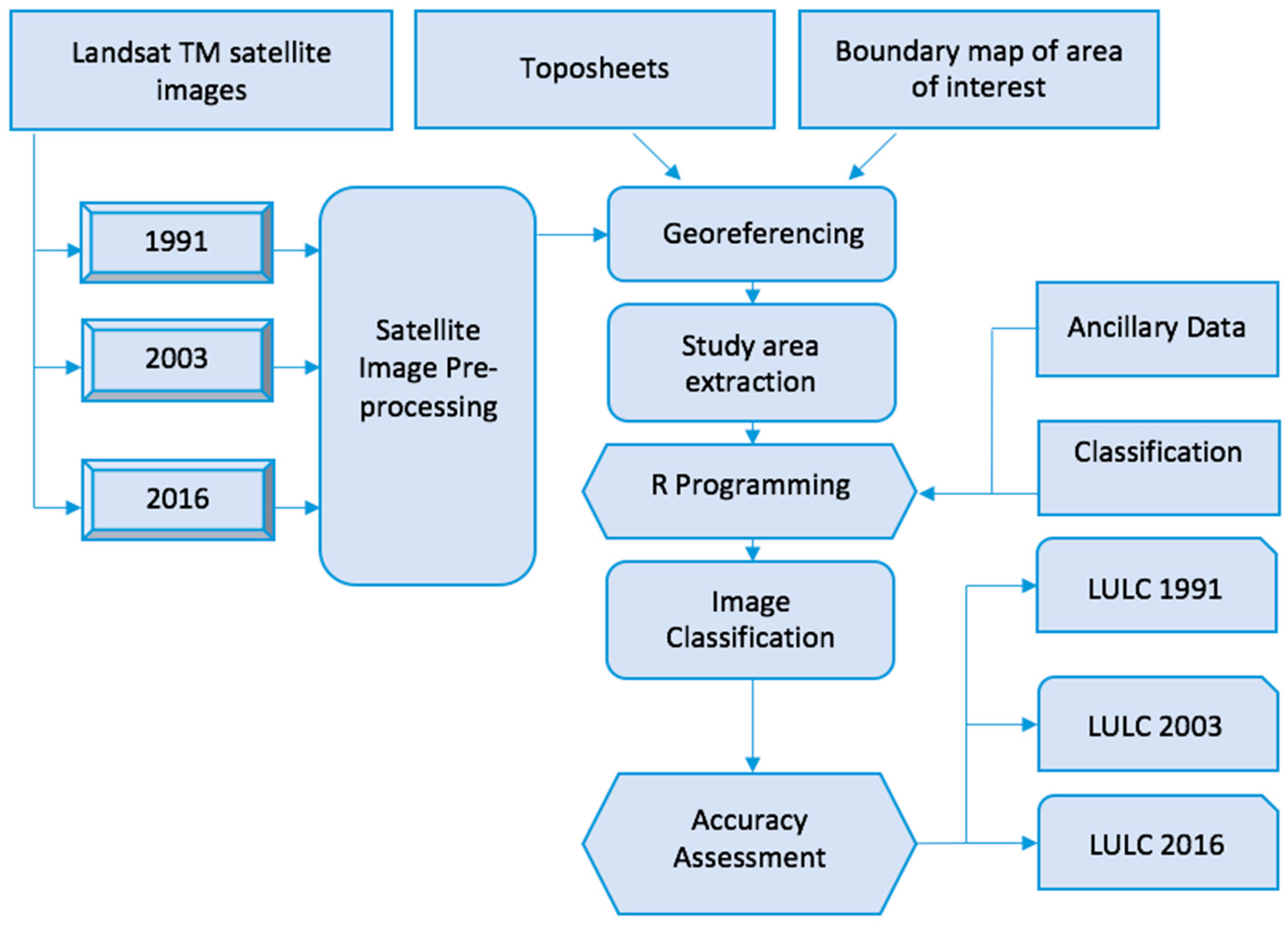
3. Materials and Methods
3.1. Data and Pre-Processing
3.2. Landuse and Landcover (LULC) Mapping, and Accuracy Assessment
- Create the stack for the available raster data;
- Create n-tree bootstrap samples from the raster data;
- Apply an unpruned classification grown for each of the bootstrap samples according to the Digital Number (DN) values of the raster data;
- Create N number of polygons according to the DN raster values;
- Assign different color bands to the several classes;
- Display the unsupervised classification.
3.3. Quantification of Extent and Level of Urban Sprawl (US)
3.3.1. Extent of US
3.3.2. Level of US
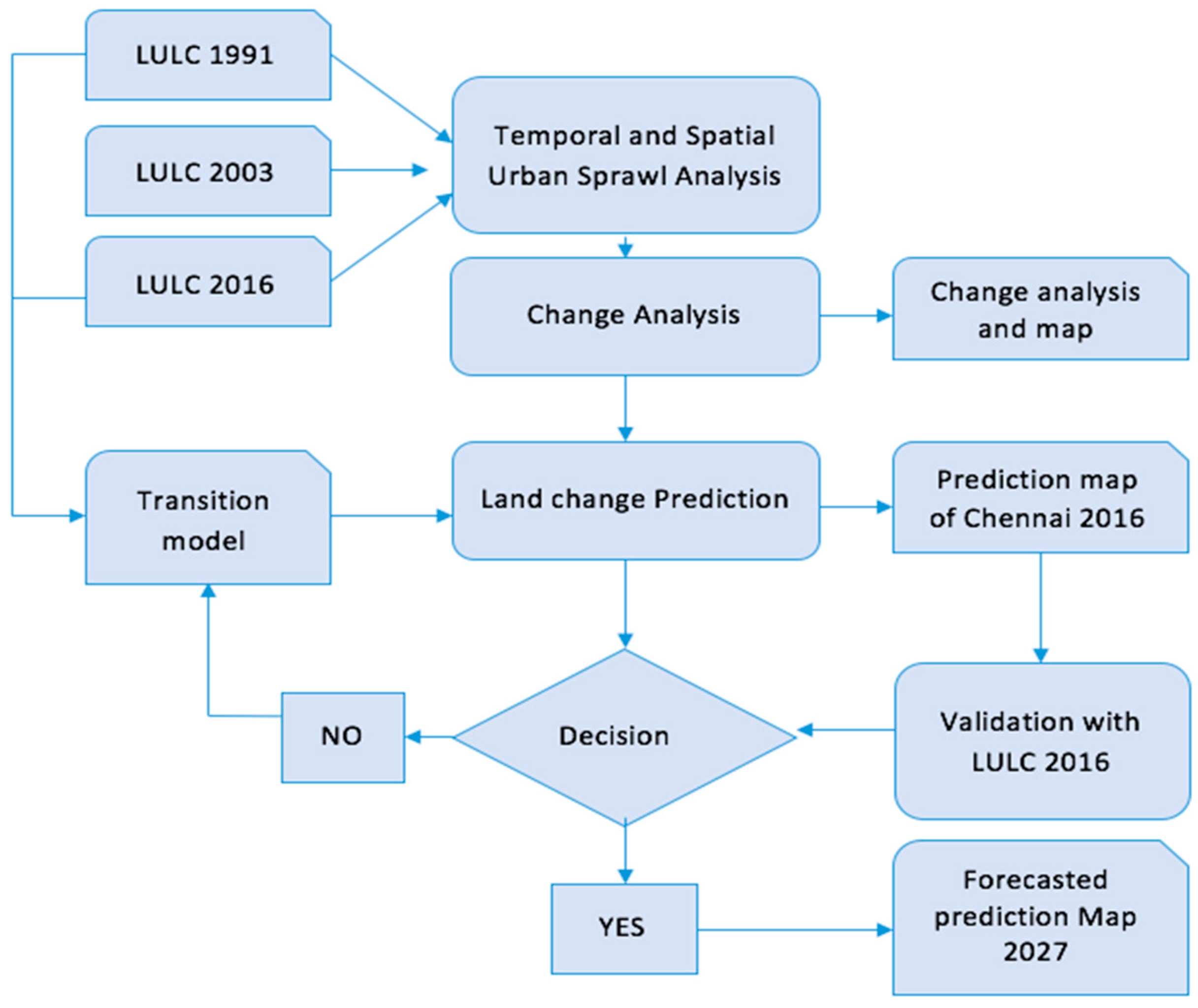
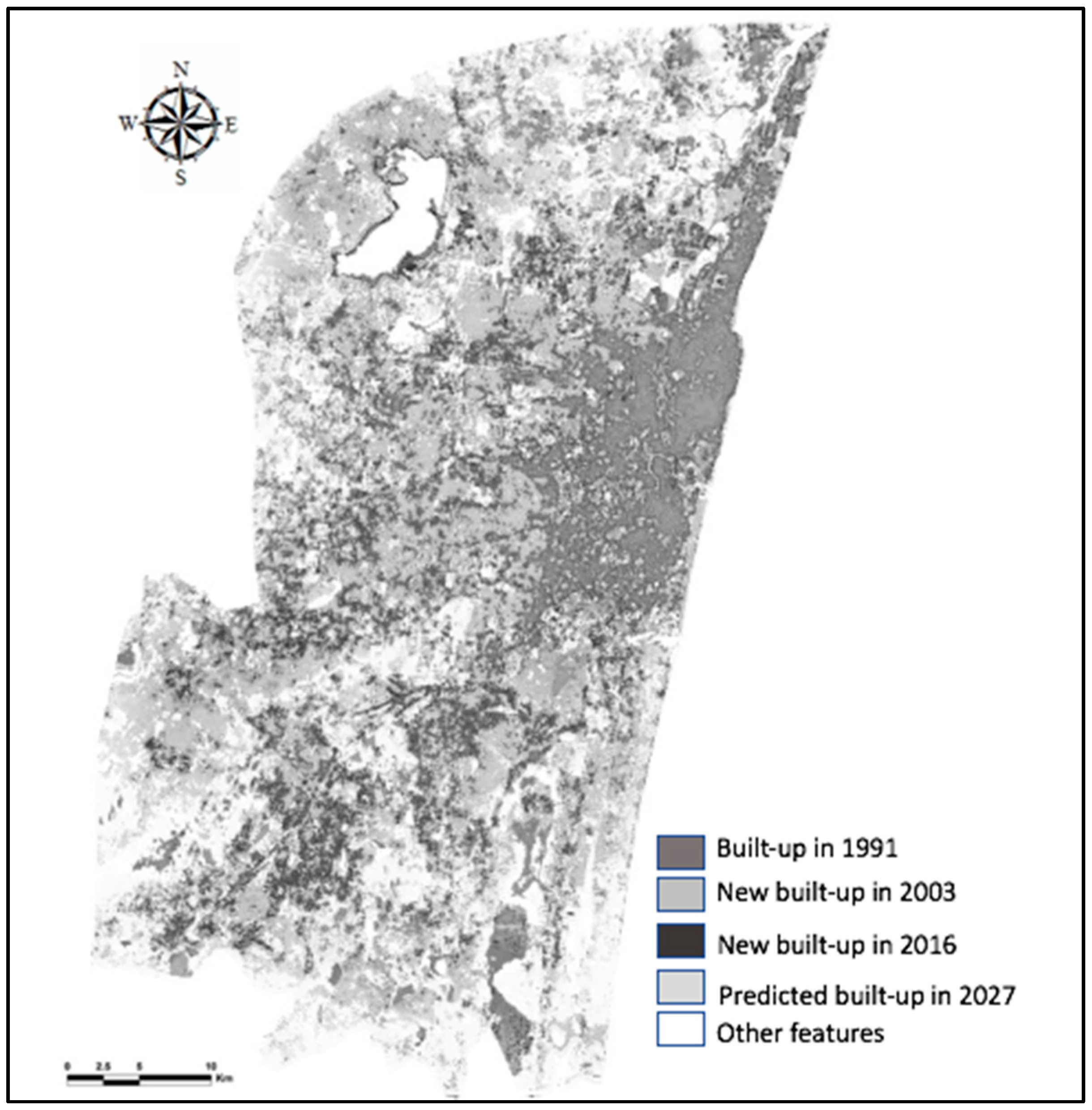
3.4. Prediction of Urban Extent for 2027
4. Results and Discussion
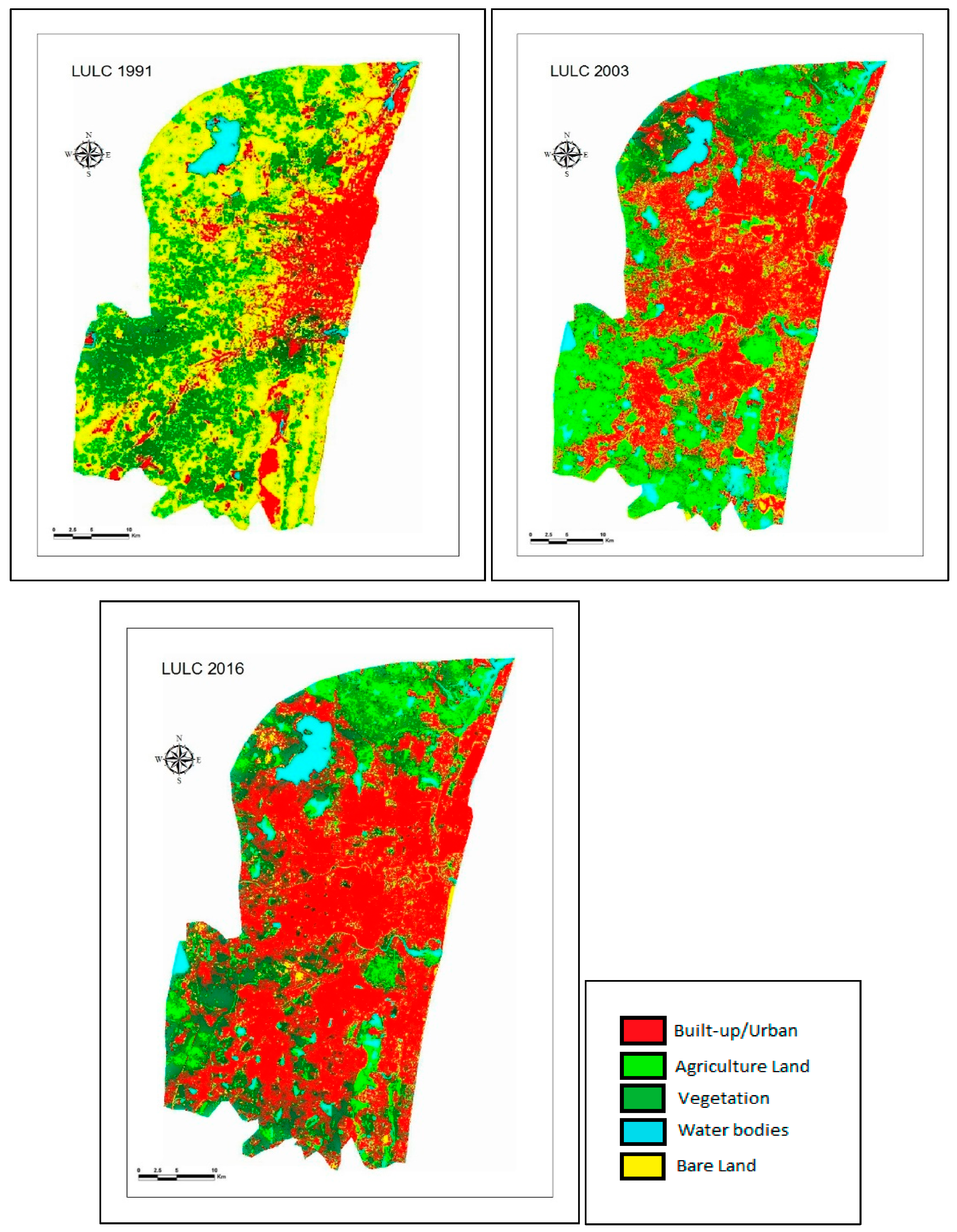
4.1. The Extent and Patterns of US in Chennai between 1991 and 2016
4.2. Change in US Level in Chennai
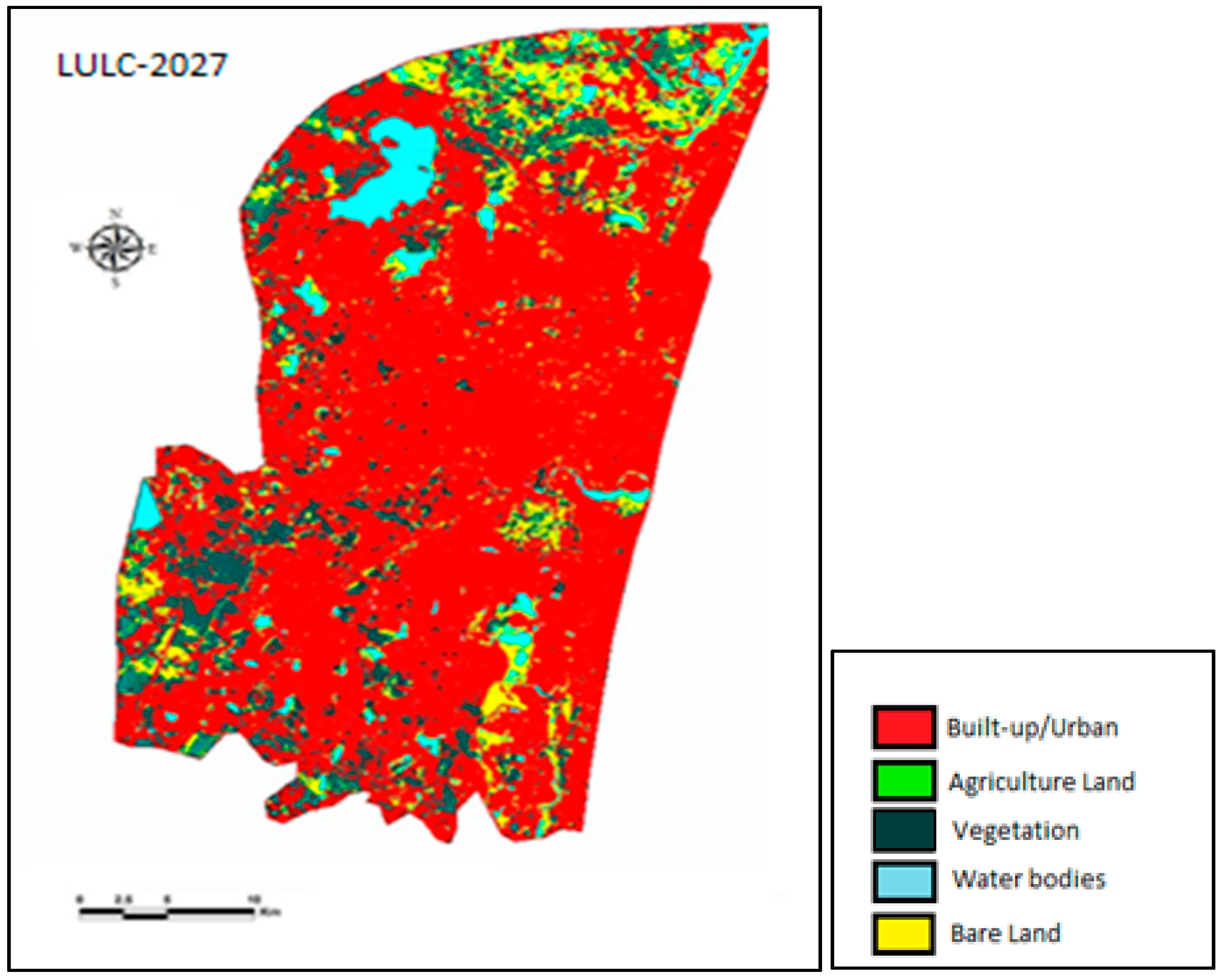
4.3. US Extent and Level Prediction for 2027
5. Concluding Remarks
Acknowledgments
Author Contributions
Conflicts of Interest
References
- Stow, D.A.; Hope, A.; McGuire, D.; Verbyla, D.; Gamon, J.; Huemmrich, F.; Houston, S.; Racine, C.; Sturm, M.; Tape, K.; et al. Remote sensing of vegetation and land-cover change in Arctic Tundra Ecosystems. Remote Sens. Environ. 2004, 89, 281–308. [Google Scholar] [CrossRef]
- Lambin, E.F.; Turner, B.L.; Geist, H.J.; Agbola, S.B.; Angelsen, A.; Folke, C.; Bruce, J.W.; Coomes, O.T.; Dirzo, R.; George, P.S.; et al. The causes of land-use and land-cover change: Moving beyond the myths. Glob. Environ. Chang. 2001, 11, 261–269. [Google Scholar] [CrossRef]
- Visalatchi, A.; Padmanaban, R. Land Use and Land Cover Mapping and Shore Line Changes Studies in Tuticorin Coastal Area Using Remote Sensing. Int. J. Remote Sens. 2012, 1, 1–12. [Google Scholar]
- Monishiya, B.G.; Padmanaban, R. Mapping and change detection analysis of marine resources in Tuicorin and Vembar group of Islands using remote sensing. Int. J. Adv. For. Sci. Manag. 2012, 1, 1–16. [Google Scholar]
- Squires, G.D. Urban Sprawl Causes, Consequences and Policy Responses; Corrier, K., Gorham, W., Hadley, J., Harrell, A.V., Reischauer, R.D., Rogers, J.R., Peterson, G.E., Nightingale, D.S., Eds.; The Urban Institute Press: Washington, DC, USA, 2002. [Google Scholar]
- Cabral, P.; Feger, C.; Levrel, H.; Chambolle, M.; Basque, D. Assessing the impact of land-cover changes on ecosystem services: A first step toward integrative planning in Bordeaux, France. Ecosyst. Serv. 2016, 22, 318–327. [Google Scholar] [CrossRef]
- Schafer, A.; Victor, D.G. The future mobility of the world population. Transp. Res. Part A Policy Pract. 2000, 34, 171–205. [Google Scholar] [CrossRef]
- Dewan, A.M.; Corner, R.J. Spatiotemporal Analysis of Urban Growth, Sprawl and Structure. In Dhaka Megacity: Geospatial Perspectives on Urbanisation, Enviornment and Health; Dewan, A., Corner, R.J., Eds.; Springer Science and Business Media: Dordretch, The Netherlands; pp. 99–121.
- Megahed, Y.; Cabral, P.; Silva, J.; Caetano, M. Land Cover Mapping Analysis and Urban Growth Modelling Using Remote Sensing Techniques in Greater Cairo Region—Egypt. ISPRS Int. J. Geo-Inf. 2015, 4, 1750–1769. [Google Scholar] [CrossRef]
- Cadenasso, M.L.; Pickett, S.T.A.; Schwarz, K. Spatial heterogeneity in urban ecosystems: Conceptualizing land cover and a framework for classification. Front. Ecol. Environ. 2007, 5, 80–88. [Google Scholar] [CrossRef]
- Zhang, Q.; Wang, J.; Peng, X.; Gong, P.; Shi, P. Urban built-up land change detection with road density and spectral information from multi-temporal Landsat TM data. Int. J. Remote Sens. 2002, 23, 3057–3078. [Google Scholar] [CrossRef]
- Luck, M.; Wu, J.G. A gradient analysis of urban landscape pattern: A case study from the Phoenix metropolitan region, Arizona, USA. Landsc. Ecol. 2002, 17, 327–340. [Google Scholar] [CrossRef]
- Cabral, P.; Santos, J.A.; Augusto, G. Monitoring Urban Sprawl and the National Ecological Reserve in Sintra-Cascais, Portugal: Multiple OLS Linear Regression Model Evaluation. J. Urban Plan. Dev. 2011, 137, 346–353. [Google Scholar] [CrossRef]
- Jayaprakash, M.; Senthil Kumar, R.; Giridharan, L.; Sujitha, S.B.; Sarkar, S.K.; Jonathan, M.P. Bioaccumulation of metals in fish species from water and sediments in macrotidal Ennore creek, Chennai, SE coast of India: A metropolitan city effect. Ecotoxicol. Environ. Saf. 2015, 120, 243–255. [Google Scholar] [CrossRef] [PubMed]
- Gowri, V.S.; Ramachandran, S.; Ramesh, R.; Pramiladevi, I.R.; Krishnaveni, K. Application of GIS in the study of mass transport of pollutants by Adyar and Cooum Rivers in Chennai, Tamilnadu. Environ. Monit. Assess. 2008, 138, 41–49. [Google Scholar] [CrossRef] [PubMed]
- Aithal, B.H.; Ramachandra, T.V. Visualization of Urban Growth Pattern in Chennai Using Geoinformatics and Spatial Metrics. J. Indian Soc. Remote Sens. 2016, 44, 617–633. [Google Scholar] [CrossRef]
- Jat, M.K.; Garg, P.K.; Khare, D. Monitoring and modelling of urban sprawl using remote sensing and GIS techniques. Int. J. Appl. Earth Obs. Geoinf. 2008, 10, 26–43. [Google Scholar] [CrossRef]
- Sudhira, H.S.; Ramachandra, T.V.; Jagadish, K.S. Urban sprawl pattern recognition and modelling using GIS. In Proceedings of the 2003 Map India, New Delhi, India, 28–30 January 2003; pp. 1–9. [Google Scholar]
- Moghadam, H.S.; Helbich, M. Spatiotemporal urbanization processes in the megacity of Mumbai, India: A Markov chains-cellular automata urban growth model. Appl. Geogr. 2013, 40, 140–149. [Google Scholar] [CrossRef]
- Dewan, A.M.; Yamaguchi, Y. Land use and land cover change in Greater Dhaka, Bangladesh: Using remote sensing to promote sustainable urbanization. Appl. Geogr. 2009, 29, 390–401. [Google Scholar] [CrossRef]
- Dewan, A.M.; Yamaguchi, Y.; Rahman, M.Z. Dynamics of land use/cover changes and the analysis of landscape fragmentation in Dhaka Metropolitan, Bangladesh. GeoJournal 2012, 77, 315–330. [Google Scholar] [CrossRef]
- Poelmans, L.; Van Rompaey, A. Computers, Environment and Urban Systems Complexity and performance of urban expansion models. Comput. Environ. Urban Syst. 2010, 34, 17–27. [Google Scholar] [CrossRef]
- Padmanaban, R. Integrating of Urban Growth Modelling and Utility Management System using Spatio Temporal Data Mining. Int. J. Adv. Earth Sci. Eng. 2012, 1, 13–15. [Google Scholar]
- Padmanaban, R. Modelling the Transformation of Land use and Monitoring and Mapping of Environmental Impact with the help of Remote Sensing and GIS. Int. J. Adv. Altern. Energy Environ. Ecol. 2012, 1, 36–38. [Google Scholar]
- Herold, M.; Goldstein, N.C.; Clarke, K.C. The spatiotemporal form of urban growth: Measurement, analysis and modeling. Remote Sens. Environ. 2003, 86, 286–302. [Google Scholar] [CrossRef]
- De Oliveira Filho, F.J.B.; Metzger, J.P. Thresholds in landscape structure for three common deforestation patterns in the Brazilian Amazon. Landsc. Ecol. 2006, 21, 1061–1073. [Google Scholar] [CrossRef]
- Tv, R.; Aithal, B.H.; Sanna, D.D. Insights to urban dynamics through landscape spatial pattern analysis. Int. J. Appl. Euarth Obs. Geoinf. 2012, 18, 329–343. [Google Scholar] [CrossRef]
- Byomkesh, T.; Nakagoshi, N.; Dewan, A.M. Urbanization and green space dynamics in Greater Dhaka, Bangladesh. Landsc. Ecol. Eng. 2012, 8, 45–58. [Google Scholar] [CrossRef]
- Ferdinent, J.; Padmanaban, R. Development of a Methodology to Estimate Biomass from Tree Height Using Airborne Digital Image. Int. J. Adv. Remote Sens. GIS 2013, 2, 49–58. [Google Scholar]
- Sabet Sarvestani, M.; Ibrahim, A.L.; Kanaroglou, P. Three decades of urban growth in the city of Shiraz, Iran: A remote sensing and geographic information systems application. Cities 2011, 28, 320–329. [Google Scholar] [CrossRef]
- Fistola, R. Urban entropy vs. sustainability: A new town planning perspective. WIT Trans. Ecol. Environ. 2012, 155, 195–204. [Google Scholar]
- Ji, W.; Ma, J.; Twibell, R.W.; Underhill, K. Characterizing urban sprawl using multi-stage remote sensing images and landscape metrics. Comput. Environ. Urban Syst. 2006, 30, 861–879. [Google Scholar] [CrossRef]
- Cabral, P.; Augusto, G.; Tewolde, M.; Araya, Y. Entropy in Urban Systems. Entropy 2013, 15, 5223–5236. [Google Scholar] [CrossRef]
- Tewolde, M.G.; Cabral, P. Urban sprawl analysis and modeling in Asmara, Eritrea. Remote Sens. 2011, 3, 2148–2165. [Google Scholar] [CrossRef]
- Fan, Y.; Yu, G.; He, Z.; Yu, H.; Bai, R.; Yang, L.; Wu, D. Entropies of the Chinese Land Use/Cover Change from 1990 to 2010 at a County Level. Entropy 2017, 19, 51. [Google Scholar] [CrossRef]
- Dewan, A.M.; Humayun, K.; Nahar, M.K.; Rahman, Z. Urbanisation and environmental degradation in Dhaka Metropolitan Area of Bangladesh. Environ. Sustain. Dev. 2012, 11, 118–147. [Google Scholar] [CrossRef]
- Shanmugam, P.; Neelamani, S.; Ahn, Y.H.; Philip, L.; Hong, G.H. Assessment of the levels of coastal marine pollution of Chennai city, Southern India. Water Resour. Manag. 2007, 21, 1187–1206. [Google Scholar] [CrossRef]
- Raman, N.; Narayanan, D.S. Impact of Solid Waste Effect on Ground Water and Soil Quality Nearer to Pallavaram Solid Waste Landfill Site in Chennai. Rasayan 2008, 1, 828–836. [Google Scholar]
- Arabindoo, P. “City of sand”: Stately Re-Imagination of Marina Beach in Chennai. Int. J. Urban Reg. Res. 2011, 35, 379–401. [Google Scholar] [CrossRef]
- Rani, C.S.S.; Rema, M.; Deepa, R.; Premalatha, G.; Ravikumar, R.; Mohan, A.; Ramu, M.; Saroja, R.; Kayalvizhi, G.; Mohan, V. The Chennai Urban Population Study (Cups)—Methodological Details—(Cups Paper No. 1). Int. J. Diabetes Dev. Ctries. 1999, 19, 149–155. [Google Scholar]
- Padmanaban, R.; Sudalaimuthu, K. Marine Fishery Information System and Aquaculture Site Selection Using Remote Sensing and GIS. Int. J. Adv. Remote Sens. GIS 2012, 1, 20–33. [Google Scholar]
- Padmanaban, R.; Thomas, V. Inventory of Liquefaction Area and Risk Assessment Region Using Remote Sensing. Int. J. Adv. Remote Sens. GIS 2013, 2, 198–204. [Google Scholar]
- Huttner, S.; Bruse, M.; Dostal, P. Using ENVI-met to simulate the impact of global warming on the mi-croclimate in central European cities. In Proceedings of the 5th Japanese-German Meeting on Urban Climatology, Freiburg im Breisgau, Germany, 6–8 October 2008; Volume 18, pp. 307–312. [Google Scholar]
- Yee, K.M.; Wai, K.P.; Jinhyung, B.; Uong, C.C. Land Use and Land Cover Mapping Based on Band Ratioing with Subpixel Classification by Support Vector Machine Techniques (A Case Study on Ngamoeyeik Dam Area, Yangon Region). J. Geol. Resour. Eng. 2016, 4, 127–133. [Google Scholar]
- Loveland, T.R.; Reed, B.C.; Brown, J.F.; Ohlen, D.O.; Zhu, Z.; Yang, L.; Merchant, J.W. Development of a global land cover characteristics database and IGBP DISCover from 1 km AVHRR data. Int. J. Remote Sens. 2000, 21, 1303–1330. [Google Scholar] [CrossRef]
- Vincenzi, S.; Zucchetta, M.; Franzoi, P.; Pellizzato, M.; Pranovi, F.; De Leo, G.A.; Torricelli, P. Application of a Random Forest algorithm to predict spatial distribution of the potential yield of Ruditapes philippinarum in the Venice lagoon, Italy. Ecol. Model. 2011, 222, 1471–1478. [Google Scholar] [CrossRef]
- Venkatesan, G.; Padmanaban, R. Possibility Studies and Parameter Finding for Interlinking of Thamirabarani and Vaigai Rivers in Tamil Nadu, India. Int. J. Adv. Earth Sci. Eng. 2012, 1, 16–26. [Google Scholar]
- Congalton, R.G. A review of assessing the accuracy of classifications of remotely sensed data. Remote Sens. Environ. 1991, 37, 35–46. [Google Scholar] [CrossRef]
- Kong, F.; Yin, H.; Nakagoshi, N. Using GIS and landscape metrics in the hedonic price modeling of the amenity value of urban green space: A case study in Jinan City, China. Landsc. Urban Plan. 2007, 79, 240–252. [Google Scholar] [CrossRef]
- UMass Landscape Ecology Lab FRAGSTATS: Spatial Pattern Analysis Program for Categorical Maps. Available online: http://www.umass.edu/landeco/research/fragstats/fragstats.html (accessed on 20 December 2016).
- Herold, M.; Scepan, J.; Clarke, K.C. The use of remote sensing and landscape metrics to describe structures and changes in urban land uses. Environ. Plan. A 2002, 34, 1443–1458. [Google Scholar] [CrossRef]
- Tsallis, C. Possible generalization of Boltzmann-Gibbs statistics. J. Stat. Phys. 1988, 52, 479–487. [Google Scholar] [CrossRef]
- Drius, M.; Malavasi, M.; Acosta, A.T.R.; Ricotta, C.; Carranza, M.L. Boundary-based analysis for the assessment of coastal dune landscape integrity over time. Appl. Geogr. 2013, 45, 41–48. [Google Scholar] [CrossRef]
- Pontius, R.G. Quantification Error Versus Location Error in Comparison of Categorical Maps. Photogramm. Eng. Remote Sens. 2000, 1610, 1011–1016. [Google Scholar]
- Pontius, R.G., Jr.; Boersma, W.; Clarke, K.; Nijs, T.; De Dietzel, C.; Duan, Z.; Fotsing, E.; Goldstein, N.; Kok, K.; Koomen, E.; et al. Comparing the input, output, and validation maps for several models of land change. Ann. Reg. Sci. 2008, 42, 11–37. [Google Scholar] [CrossRef]
- Martins, V.N.; Cabral, P.; Silva, D.S. System Sciences Urban modelling for seismic prone areas: The case study of Vila Franca do Campo (Azores Archipelago, Portugal). Nat. Hazards Earth Syst. Sci. 2012, 12, 2731–2741. [Google Scholar] [CrossRef]
- Zyczkowski, K. Renyi extrapolation of Shannon entropy. Open Syst. Inf. Dyn. 2003, 10, 297–310. [Google Scholar] [CrossRef]
- Langley, S.K.; Cheshire, H.M.; Humes, K.S. A comparison of single date and multitemporal satellite image classifications in a semi-arid grassland. J. Arid Environ. 2001, 49, 401–411. [Google Scholar] [CrossRef]
- Araya, Y.H.; Cabral, P. Analysis and modeling of urban land cover change in Setúbal and Sesimbra, Portugal. Remote Sens. 2010, 2, 1549–1563. [Google Scholar] [CrossRef]
- Chaves, A.B.; Lakshumanan, C. Remote Sensing and GIS-Based Integrated Study and Analysis for Mangrove-Wetland Restoration in Ennore Creek, Chennai, South India. In Proceedings of the Taal2007: The 12th World Lake Conference, Jaipur, India, 29 October–2 November 2008; pp. 685–690. [Google Scholar]
- Tanaka, N. Vegetation bioshields for tsunami mitigation: Review of effectiveness, limitations, construction, and sustainable management. Landsc. Ecol. Eng. 2009, 5, 71–79. [Google Scholar] [CrossRef]
- Kerr, A.M.; Baird, A.H.; Bhalla, R.S.; Srinivas, V. Reply to “Using remote sensing to assess the protective role of coastal woody vegetation against tsunami waves”. Int. J. Remote Sens. 2009, 30, 3817–3820. [Google Scholar] [CrossRef]
- Dhorde, A.; Gadgil, A. Long-term temperature trends at four largest cities of India during the twentieth Century. J. Ind. Geophys. Union 2009, 13, 85–97. [Google Scholar]
- Kim Oanh, N.T.; Upadhyay, N.; Zhuang, Y.H.; Hao, Z.P.; Murthy, D.V.S.; Lestari, P.; Villarin, J.T.; Chengchua, K.; Co, H.X.; Dung, N.T.; et al. Particulate air pollution in six Asian cities: Spatial and temporal distributions, and associated sources. Atmos. Environ. 2006, 40, 3367–3380. [Google Scholar] [CrossRef]
- Chithra, V.S.; Shiva Nagendra, S.M. Indoor air quality investigations in a naturally ventilated school building located close to an urban roadway in Chennai, India. Build. Environ. 2012, 54, 159–167. [Google Scholar] [CrossRef]
- Padmanaban, R.; Kumar, R. Mapping and Analysis of Marine Pollution in Tuticorin Coastal Area Using Remote Sensing and GIS. Int. J. Adv. Remote Sens. GIS 2012, 1, 34–48. [Google Scholar]
- Giridharan, L.; Venugopal, T.; Jayaprakash, M. Evaluation of the seasonal variation on the geochemical parameters and quality assessment of the groundwater in the proximity of River Cooum, Chennai, India. Environ. Monit. Assess. 2008, 143, 161–178. [Google Scholar] [CrossRef] [PubMed]
- Vasanthi, P.; Kaliappan, S.; Srinivasaraghavan, R. Impact of poor solid waste management on ground water. Environ. Monit. Assess. 2008, 143, 227–238. [Google Scholar] [CrossRef] [PubMed]


| Date | Sensor | Path/Row |
|---|---|---|
| 25 August 1991 | Landsat-5 TM | 142/51 |
| 9 May 2003 | Landsat-7 ETM+ | 142/51 |
| 4 July 2016 | Landsat-7 ETM+ | 142/51 |
| No | LULC Classes | Land Uses Included in the Class |
|---|---|---|
| 1 | Water bodies | Rivers, reservoir, lakes, streams, open water, and ponds |
| 2 | Urban | Roads, airports, and built-up areas |
| 3 | Agriculture | Agriculture lands and plantations |
| 4 | Bare land | Dry lands, non-irrigated lands, ready for construction, and real estate plots |
| 5 | Vegetation | Forests and shrubs |
| Landscape Metrics | Formula | Description | Range |
|---|---|---|---|
| Class Area Metrics (CA) | aij = area in m2 of patch ij. | Total amount of class area in the landscape | CA > 0, without limit |
| Number of Patches (NP) | ni = total number of patches in the area of patch type i (class). | Number of patches of landscape classes (Built up and non-built-up) | NP ≥ 1, without limit |
| Largest patch Index (LPI) | aij = area in m2 of patch ij and A = landscape area in total (m2) | Percentage of the landscape included by the largest patch | 0 < LPI ≤ 100 |
| Clumpiness Index (CLUMPY) | < 5, else ] gii = number of like joins among pixels of patch type, i based double-count process and gik = number of like joins among pixels of patch type, k based double-count process, Pi = amount of the landscape occupied by patch type | Measure the clumpiness of patches in urban areas | −1 ≤ CLUMPY ≤ 1 |
| Fractal Index Distribution (FRAC_AM) | aij = area in m2 of patch ij. | To measure area weighted mean patch fractal dimension | 1 ≤ FRAC_AM ≤ 2 |
| Contagion | pi = amount of the landscape employed by patch type (i) class and gik = number of like joins among pixels of patch type, i and k based double-count process, m = number of patch classes (types) existing in the landscape | Defines the heterogeneity of a landscape | Percent < Contagion ≤ 100 |
| Metrics | Year | Changes in Urban Structure | ||||
|---|---|---|---|---|---|---|
| 1991 | 2003 | 2016 | Δ% = 1991–2003 | Δ% = 2003–2016 | Δ% = 1991–2016 | |
| CA | 20,110.61 | 39,965.51 | 58,030.42 | 98.72 | 45.20 | 188.5 |
| NP | 289 | 354 | 477 | 22.49 | 34.74 | 65 |
| LPI | 2.14 | 4.87 | 6.78 | 127.57 | 39.21 | 216.8 |
| Clumpy | −1 | 0.6 | 0.8 | 160 | 33.33 | 180 |
| FRAC_AM | 1.12 | 1.27 | 1.83 | 13.39 | 44.09 | 63.3 |
| CONTAG | 72.32 | 68.43 | 71.24 | 6.66 | 4.10 | 1.4 |
| Land-Use Class | 1991 | 2003 | 2016 | 2027 | Forecasted LULC in 2027 | |
|---|---|---|---|---|---|---|
| ha | % | |||||
| Built-up/urban | 20,110.61 | 39,965.51 | 58,030.42 | 70,836.76 | 12,805.58 | 22.06 |
| Agriculture | 9387.15 | 22,857.47 | 5584.44 | 701.35 | −4883.09 | −87.44 |
| Vegetation | 21,677.89 | 9296.41 | 11,754.56 | 3961.66 | −7792.9 | −66.29 |
| Water bodies | 5320.48 | 6772.27 | 6120.62 | 5420.62 | −700 | −11.43 |
| Bare land | 25,992.02 | 3596.48 | 998.10 | 1570.12 | 572.02 | 57.31 |
| Total | 82,488.16 | 82,488.16 | 82,488.16 | 82,488.16 | - | - |
© 2017 by the authors. Licensee MDPI, Basel, Switzerland. This article is an open access article distributed under the terms and conditions of the Creative Commons Attribution (CC BY) license (http://creativecommons.org/licenses/by/4.0/).
Share and Cite
Padmanaban, R.; Bhowmik, A.K.; Cabral, P.; Zamyatin, A.; Almegdadi, O.; Wang, S. Modelling Urban Sprawl Using Remotely Sensed Data: A Case Study of Chennai City, Tamilnadu. Entropy 2017, 19, 163. https://doi.org/10.3390/e19040163
Padmanaban R, Bhowmik AK, Cabral P, Zamyatin A, Almegdadi O, Wang S. Modelling Urban Sprawl Using Remotely Sensed Data: A Case Study of Chennai City, Tamilnadu. Entropy. 2017; 19(4):163. https://doi.org/10.3390/e19040163
Chicago/Turabian StylePadmanaban, Rajchandar, Avit K. Bhowmik, Pedro Cabral, Alexander Zamyatin, Oraib Almegdadi, and Shuangao Wang. 2017. "Modelling Urban Sprawl Using Remotely Sensed Data: A Case Study of Chennai City, Tamilnadu" Entropy 19, no. 4: 163. https://doi.org/10.3390/e19040163
APA StylePadmanaban, R., Bhowmik, A. K., Cabral, P., Zamyatin, A., Almegdadi, O., & Wang, S. (2017). Modelling Urban Sprawl Using Remotely Sensed Data: A Case Study of Chennai City, Tamilnadu. Entropy, 19(4), 163. https://doi.org/10.3390/e19040163