1. Introduction
In transportation, travel time is confined to the time traveled by vehicles in a road network. Accordingly, travel time forecast is to predict the time taken by a vehicle to travel between any two points in a road network, which may benefit transportation planning, design, operations, and evaluation [
1]. With ever-increasing traffic congestion in metropolitan areas, travel time for every traveler becomes complicated and irregular. How to accurately predict travel time, therefore, is of great importance to researchers. In the past few decades, a variety of travel time prediction approaches has been developed such as the linear regression,
ARIMA, Bayesian nets, neural networks, decision trees, support vector regression and Kalman filtering methods. Based on periodic fluctuations of historical travel time series, these approaches make use of their own derivation rules to recognize traffic patterns and predict future travel time on specific routes as precisely as possible. However, the inevitable nonstationarity of travel time series caused by high self-adapting and heterogenetic drivers or by unpredictable and unusual circumstances makes it difficult to accurately predict future travel time. In addition to the performance of prediction models, the quality of input data (historical travel time series) for prediction model affects the precision of travel time prediction.
Nowadays, various data are employed for travel time prediction [
2,
3,
4], e.g., vehicle trajectory data, mobile phone data, smart card data, loop detector data, video monitoring data, and artificial statistical data. Vehicle trajectory data are frequently collected from a large number of vehicles and consist of a huge number of GPS sample points including geographic coordinates and sample time as well as the identification of vehicle. Historical travel time series in specific trips can be extracted from large amounts of vehicle trajectory data, and travel time prediction can be achieved. Based on vehicle trajectory data, many existing research works have been performed for travel time prediction. Some of them evaluate the performance of prediction models [
3,
5,
6,
7], and some of them focus on the reliability or uncertainty of historical travel time series [
8,
9,
10,
11,
12,
13], but few of them examine the quality of data from the perspective of prediction.
Travel time reliability is the consistency or dependability in travel times as measured day-to-day or at different times of a day [
14], which represents the temporal uncertainty experienced by travelers in their trip [
15] or the travel time distributions under various external conditions [
16]. Travel time reliability only presents the certainty of historical travel rules but not the accuracy of future travel times.
The aim of this paper is to evaluate the effectiveness of historical travel time series extracted from vehicle trajectory data in travel time prediction. Especially, we use the term “predictability” to denote the results of evaluation. In traffic studies, some research efforts about predictability have been presented. Yue et al. [
17] used the cross-correlation coefficient between traffic flows collected at two detector stations to explain short-term traffic predictability in the form of probability. Foell et al. [
18] analyzed the temporal distribution of ridership demand on various date conditions and used the F-score, an effective metric of information retrieval, to measure the predictability of bus line usage. Siddle [
19] introduced the travel time predictability of two specific prediction models—auto-regressive moving average and non-linear time series analysis—in the Auckland strategic motorway network; and travel time predictability was used to explain the performance of specific prediction models. In addition, the predictability of road section congestion (speed) [
20] and human mobility [
21,
22] are measured by information entropy. Until now, there is not enough literature on data-driven measurement of travel time predictability. Therefore, we hope to explore travel time predictability for evaluating the characteristic of travel time series on prediction.
In this paper, travel time predictability describes the possibility of correct time prediction based on historical travel time series. It indicates the influence of the complexity of historical travel time series on prediction results. For example, travel time predictability of a travel time series being 0.9 indicates that the travel time prediction accuracy cannot exceed 90% for the given travel time series no matter how good a predictive model is. Regular commute patterns give us confidence about future travel times, but random traffic flow often disturbs traffic rules and bring uncertain changes to travel time prediction.
Song et al. [
22] explored the limits of predictability of human mobility and developed a method to measure the upper bound of predictability based on information entropy [
23] and Fano’s inequality [
24]. In their research, mobile phone data were employed to quantify human mobility as discrete location series, and the entropy of location series was measured by Lempel-Ziv data compression [
25]; Fano’s inequality was used to deduce the relationships between entropy and the upper bound of predictability. A Lempel-Ziv data compression algorithm is a method to measure the complexity of the nonlinear symbolic coarse-grained time series. However, travel time series usually has a continuous range of values determined by the tradeoff between accuracy and grain size. Since the complexity of time series is highly sensitive to grain size [
26], the symbolization of travel time series is never a straightforward task. Furthermore, the complexity of the Lempel-Ziv algorithm can only be used for qualitative analysis and is not suitable for quantitative description [
27]. Therefore, the Lempel-Ziv algorithm is not suitable for measuring the complexity of travel time series, and the method proposed by Song et al. [
22] is not applicable to travel time predictability.
Inspired by Song et al. [
22], this paper attempts to measure the complexity of travel time series and assess travel time predictability. First, a travel time series is defined as a continuous variable, and multiscale entropy (
MSE) [
28] in different scales is measured to present the true entropy of the given travel time series. Then, the upper bound of predictability is calculated based on the method of Song et al. [
22]. Usually,
MSE is used to assess the complexity of multi-value time series from the perspective of multi-time scales and has been successful in many fields. However,
MSE often produces some inaccurate estimations or undefined entropy which could largely bias the evaluation of the complexity of travel time series. Wu et al. [
29] proposed the refined composite multiscale entropy (
RCMSE) algorithm based on
MSE, and found that
RCMSE increases the accuracy of entropy estimation and reduces the generation of undefined entropy.
To this end, our contributions are to integrate the two methods proposed by Wu et al. [
29] and Song et al. [
22], and apply them to evaluate the features of entropy and predictability of travel time series.
This paper applies the above techniques to an express road section with heavy traffic flow in Shanghai, China. Taxi cab trajectory data recorded in April 2015 are used to present the average taxi mobility trends and evaluate travel time predictability. Commonly seen mobility research often focuses on the mobility patterns of independent individuals (person or vehicle) based on such as mobile phone data [
22,
30,
31] and GPS data [
22,
32,
33]. Differently, travel time predictability emphasizes the expected success rate of travel time prediction based on a given travel time series from individual or statistics values of travel time, and the statistical trends of travel times from multiple vehicles may present traffic patterns more effectively than individual mobility which may be affected by unpredictable driving behaviors. In this paper, massive trip data in one route are acquired from a large amount of taxi trajectory data, and the 5 min travel time series is averaged to present the statistical trends of travel time. We then assess the entropy and predictability based on the travel time series. Next, we discuss the influences of time scales, tolerance, and series length on entropy and travel time predictability. Finally, we employ two prediction models,
ARIMA and
BPNN, to predict the future travel time of the selected route for model validation.
The rest of this paper is organized as follows. The next section defines the methodology of travel time predictability. The study area, data sources and results of a case study are presented in
Section 3.
Section 4 concludes the paper.
2. Materials and Methods
Historical travel time series are extracted from vehicle trajectory data and include a large number of sample points. Each sample trajectory consists of a vehicle ID, a time stamp, longitude, latitude, speed, etc. To attain the travel time of a specific trip, road matching of vehicle trajectory data is performed to specific routes using the method proposed by Li et al. [
34]. By calculating the difference in the time stamp of the first and last sample points of origin and destination of a given trip, the set of travel times for all trips is established. Then, based on a predefined departure time interval, the travel times of all trips that fall into the departure time interval are averaged to generate travel time series.
For any travel time series with the same routes, we employ the
RCMSE algorithm [
29] to calculate their multiscale entropy values and evaluate the complexity. Then, travel time predictability is defined, and the relationship between the upper bound of travel time predictability and the entropy of the historical travel time series is presented.
2.1. Entropy of Travel Time Series
Multiscale entropy of the travel time series is measured by the refined composite multiscale entropy (RCMSE) algorithm.
Let denote a travel time series.
Step 1. Construct
-dimensional vectors
by using Equation (1).
Step 2. Calculate the Euclidean distance
between any two vectors
and
by using Equation (2).
Step 3. Let be the tolerance level. If , and are called an -dimensional matched vector pair. represents the total number of -dimensional matched vector pairs. Similarly, is the total number of ()-dimensional matched vector pairs.
Step 4. The sample entropy (
SampEn) is defined by Equation (3).
Step 5. Let
be the
-th coarse-grained time series of
defined in Equation (4), where
is the length of the coarse-grained time series, and
is a scale factor. To obtain
, the original time series
is segmented into
coarse-grained series with each segment with a length
. The
-th element of the
-th coarse-grained time series
is the mean value of each segment
of the original time series
.
Step 6. Classical multiscale entropy,
, is defined by Equation (5).
Step 7.
RCMSE is defined in Equation (6), where
is the total number of
-dimensional matched vector pairs in the
-th coarse-grained time series with a length of
.
Compared with
SampEn and
MSE which are more likely to induce undefined entropy, the
RCMSE algorithm can estimate entropy more accurately. In Equation (7), the true entropy
of the travel time series
is denoted by
.
is roughly equal to, with time scale
, the negative logarithm of the mean of the conditional probability of new patterns (i.e., the distance between vectors is greater than
) when the dimension of the pattern changes (i.e.,
to
).
describes the degree of irregularity of the travel time series at different time scales and is proportional to the complexity of the travel time series. Based on Equation (7), the true entropy of the travel time series with different time scales can be achieved.
2.2. Travel Time Predictability
Based on the historical travel time series, the predictability of travel time is defined as the probability
that an algorithm can correctly predict future travel time. Again,
represents a historical travel time series,
is the actual travel time of the
,
is the expected value, and
is the estimated value based on model
. Let
be the probability of
with a given historical travel time series
. Equation (8) shows that
is the random value of distribution of the subsequent travel time and it is an upper bound of the probability distribution of predictive values. In other words, any prediction based on historical series
cannot do better than the one having the true travel time being equal to the expected value,
.
The definition of predictability
for a travel time series with a length of
is given by Equation (9), where
is the probability of observing a particular historical travel time series
.
presents the best success rate to predict the
travel time based on
.
can be viewed as the averaged predictability (Song et al., 2010) of a historical travel time series.
Next, we relate entropy
to predictability
to explore the upper bound of predictability
. Based on Fano’s inequality [
24], the relationship between entropy and predictability is shown in Equation (10), which indicates that the complexity of
is less than or equal to the sum of the complexity of successfully predicting
and the complexity of failing to predict
, where
is the number of values of
. Travel time is defined in second and
denotes the total time (seconds) of
. The equality in Equation (10) holds up when
meets the maximum value
.
is presented in Equation (11) and its relationship with the upper bound of travel time predictability is presented in Equation (12). Based on the known
in Equation (7), we can traverse from 0 to 1 to achieve the optimal solution of
with a given accuracy target.
3. Experiments
3.1. Study Area and Data
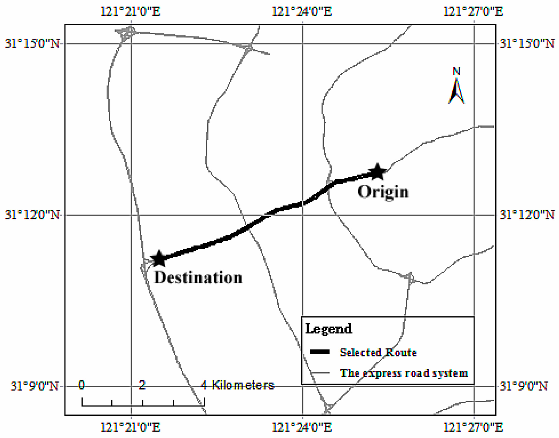
An express road section (about 6.74 km) in Shanghai, China is selected as the study area. As shown in
Figure 1, the selected route is a traffic corridor with heavy traffic and is a part of the express road system of Shanghai represented by gray lines. Since this area includes the closed road segments, continuous traffic flow will not be interrupted by an intersection’s delay, and the fluctuations of travel time coincide with traffic patterns.
Taxi cab trajectory data associated with the selected route in April 2015 are extracted as the real travel time series. Note that we only use the trips occupied by passengers and discard the patrolling ones (a state of seeking clients in the street). Each trip consists of an origin, a destination, and a route. The total number of passenger trips is 20,430, and averages about 29 per hour, which is sufficient to represent the dynamics of travel time. In addition to the route length, the travel time of a taxi cab trajectory may also be affected by heterogeneous driving behavior, therefore, the distribution of travel time derived from individual trips could be rather complex [
6,
30,
32]. Instead, the travel time estimated from multiple vehicles can well reflect the average trend of travel time and hence more effectively characterize traffic patterns than individual mobility. We use a 5 min time interval to the average travel time of travel cases to obtain a 5 min travel time series from taxi cab trajectory data in April 2015.
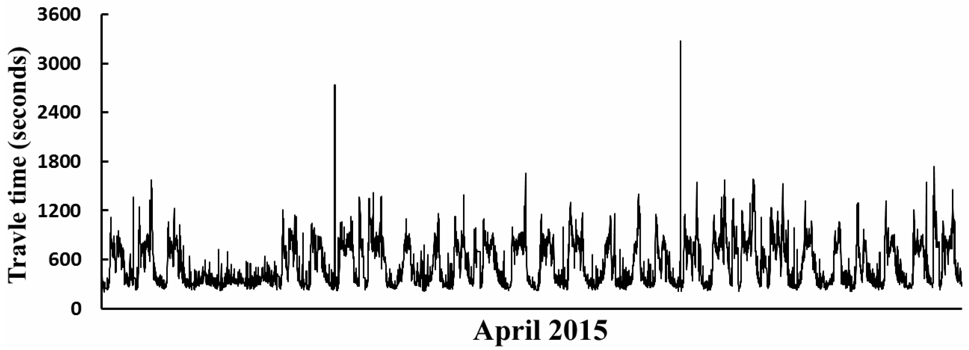
Figure 2 shows the 5 min travel time series with 8,640 sample GPS points. Let
depict the 5 min travel time series, where
is the
i-th sample point, and
is the number of points of
.
Given that the key of this paper is to analyze travel time predictability from the aspect of prediction, the average taxi mobility trends are presented by the 5 min travel time series and have nothing to do with individual taxi behavior. The analysis and evaluation of entropy and predictability are given below.
3.2. Entropy and Predictability
To evaluate the complexity of travel time series, the daily entropy, named , and the weekly entropy, named , are calculated with 24-hour subseries, i.e., 288 consecutive points, and 168 h (7 days) subseries, i.e., 2016 consecutive points, respectively, from the 5 min travel time series. We set the difference of adjacent subseries is 1 h (12 points) to obtain many subseries. Then, we let , where is a subset of with 288 consecutive points, and we let , where is a subset of with 2016 consecutive points.
Let scale factor
, tolerance r
, and dimension
, where
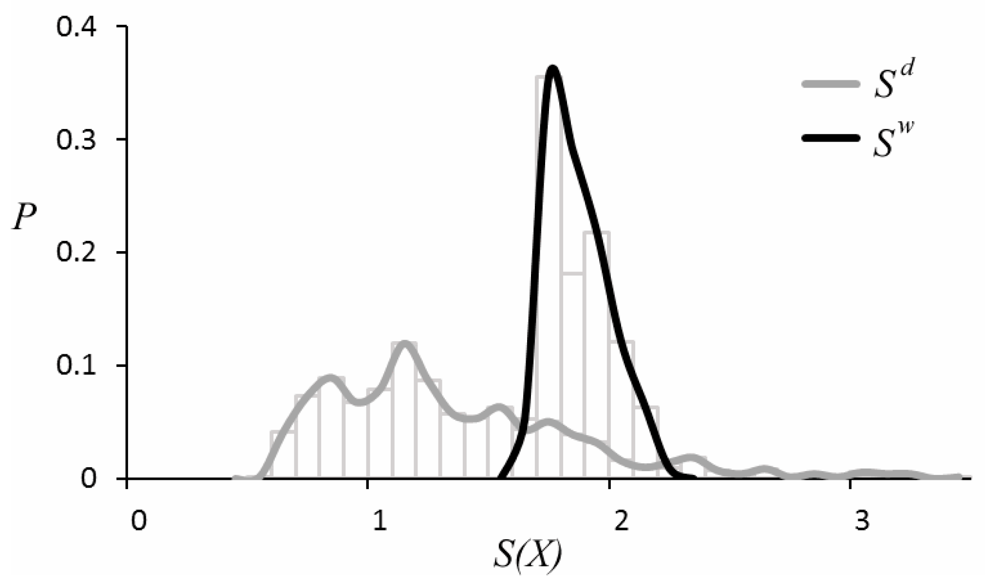
is the standard deviation of the 5 min travel time series. The statistical results of values of
and
are shown in
Figure 3. It can be seen that the values of
are scattered in the range of 0.6–3.4 and the values of
are compact in the range of 1.6–2.3. The remarkable difference between
and
means that the complexity of daily travel time series tends to change frequently; by contrast, the complexity of weekly travel time series is stable.
peaks at about 1.7, indicating that, on average, the probability of new 2-dimension (
) patterns in a weekly travel time series is
.
peaks at about 1.2, and the probability of new patterns in a daily travel time series is
indicating that weekly travel time series with greater complexity have lower probability of new patterns than relatively simple daily travel time series.
Travel time predictability is the probability of an accurate prediction, which is determined by the complexity (entropy) and the range of the travel time series. In our experiments, we set the accuracy of 0.001 to calculate the upper bound of travel time predictability by Equation (12). Therefore, the optimal (maximum) can be achieved by traversing in the range of 0.001–0.999.
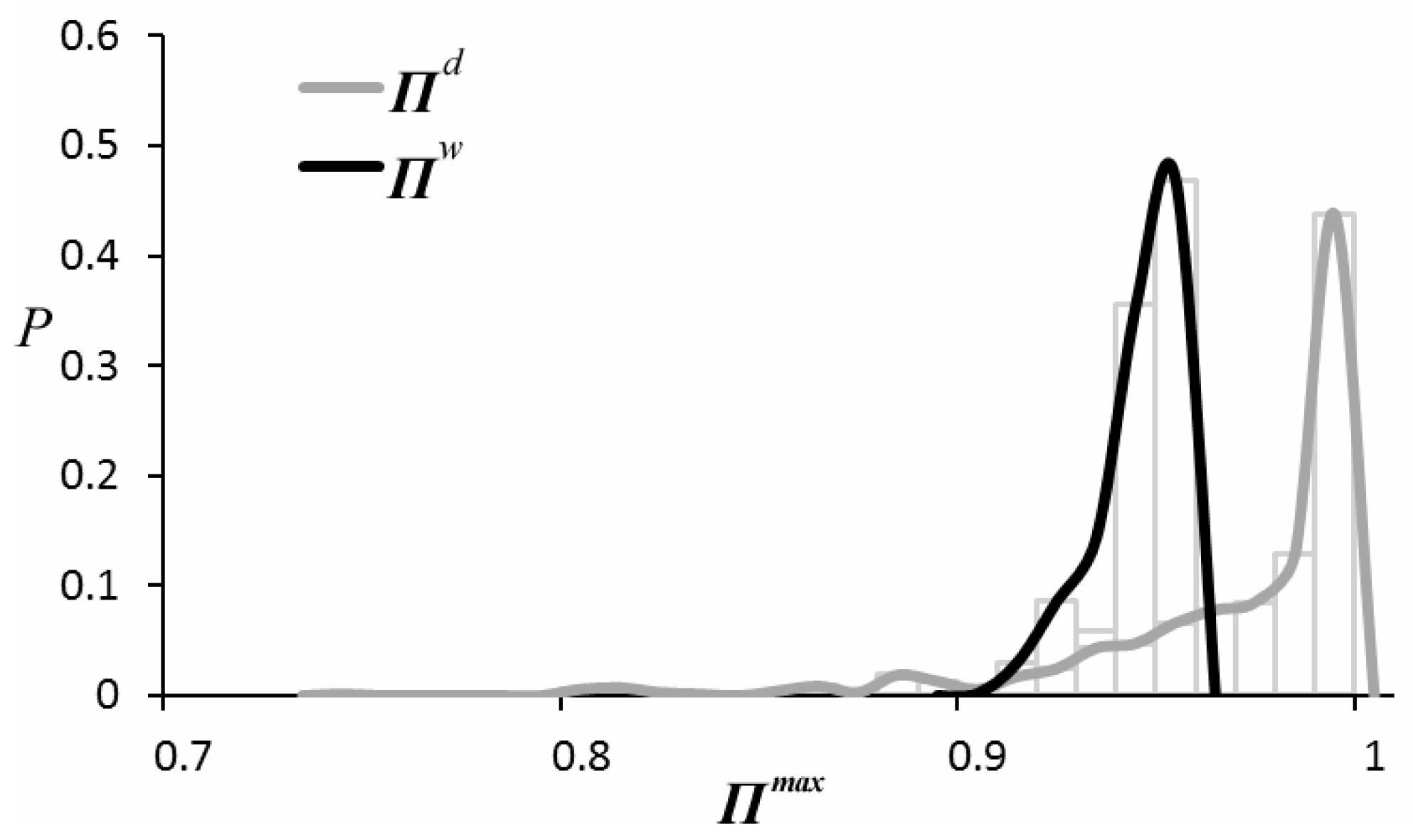
The statistical results of the upper bound of travel time predictability in weekly travel time series
and daily travel time series
are shown in
Figure 4. Since travel time predictability is influenced by entropy and the range of series, weekly travel time series with higher entropy have lower predictability, peaking at 0.95, and daily travel time series with lower entropy have higher predictability, peaking at 0.99. This demonstrates that the more complex the travel time series is, the less predictability it is, in other words, the less likely to correctly predict it.
3.3. Analysis and Discussion
As formulated in Equations (7) and (12), the features of travel time predictability are influenced by three key factors, i.e., scale factor , tolerance , and series length. In this subsection, we analyze the effectiveness of these factors to the predictability of travel time series, and discuss the features and trends of . The validity of the proposed travel time predictability is verified by comparing and the prediction results of future travel time from two typical prediction models, ARIMA and BPNN.
3.3.1. Time Scales
The scale factor
is the key parameter of
RCMSE. It can be used to analyze the complexity and predictability of travel time series in multiple time scales.
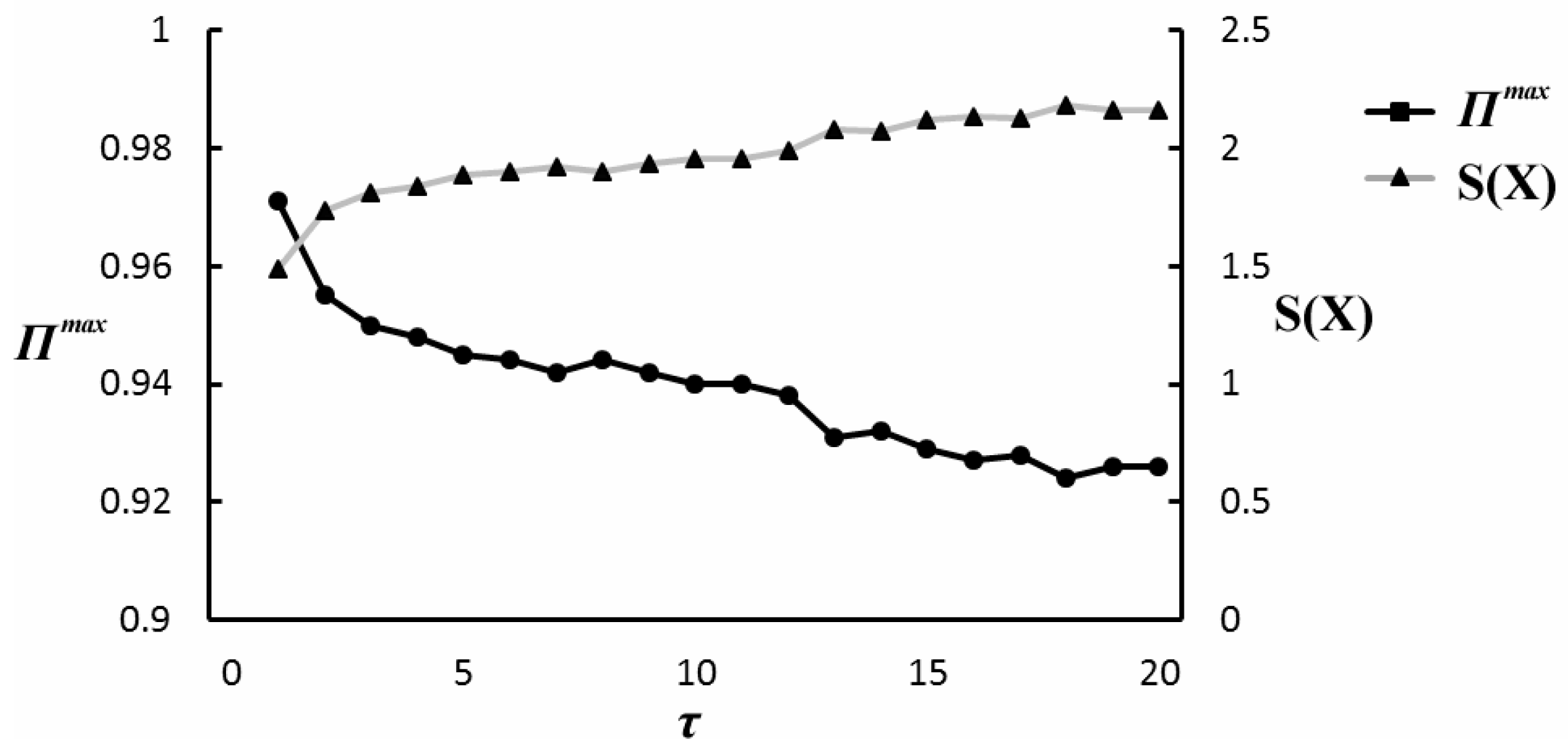
Figure 5 shows the entropy and predictability of 5 min travel time series with time scales of 1–20. The entropy is calculated by Equation (7) with
, and
.
is calculated by Equation (12). As
increases, entropy rises and predictability falls. There are more “new patterns” in the travel time series of longer time scales. The complexity of the travel time series of longer time scales is greater than those of shorter time scales, and the travel time series of longer time scales are more difficult to correctly predict.
3.3.2. Tolerance
Tolerance
, is a key factor in evaluating the complexity of travel time series and constrains the contributions of travel time fluctuations to the complexity. We attempt to evaluate the effectiveness of
in six time scales, i.e.,
= 2, 4, 6, 8, 10, and 12.
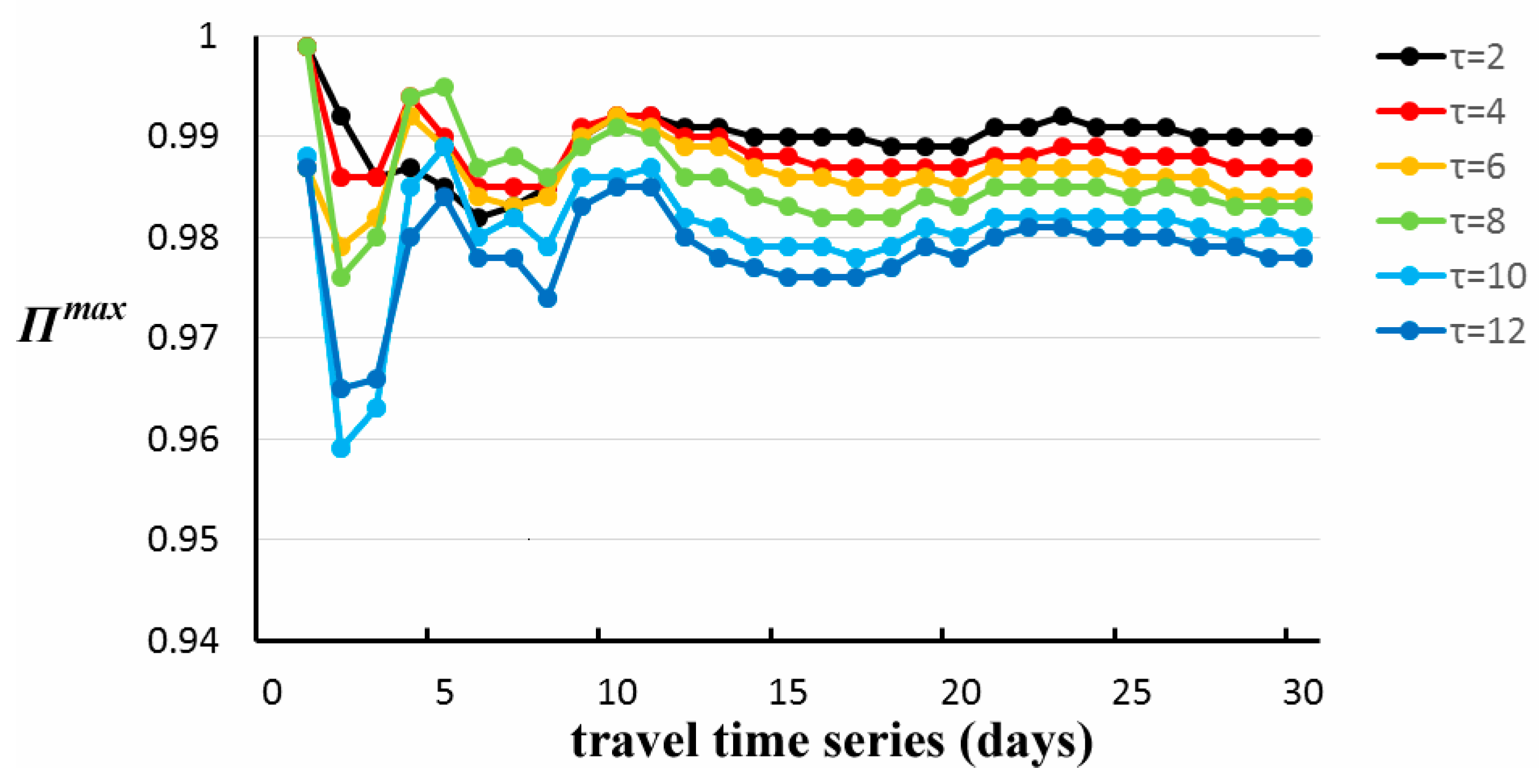
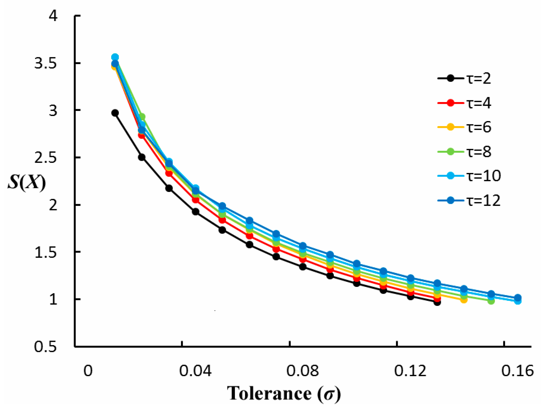
Figure 6 and
Figure 7 show the changing trends of entropy and travel time predictability of the 5 min travel time series with
of
to
, respectively. Since the travel time predictability of six time scales reaches the maximum value 0.999 when
is equal to
, the test range of
is
to
. In
Figure 6, with the increase in
, the entropy gradually becomes lower because the value gap between travel times less than
is not concerned. To six time scales, in addition to
= 2, other values of entropy are hard to distinguish at a lower
, and ordered values of entropy can be found at higher
values (about
to
).
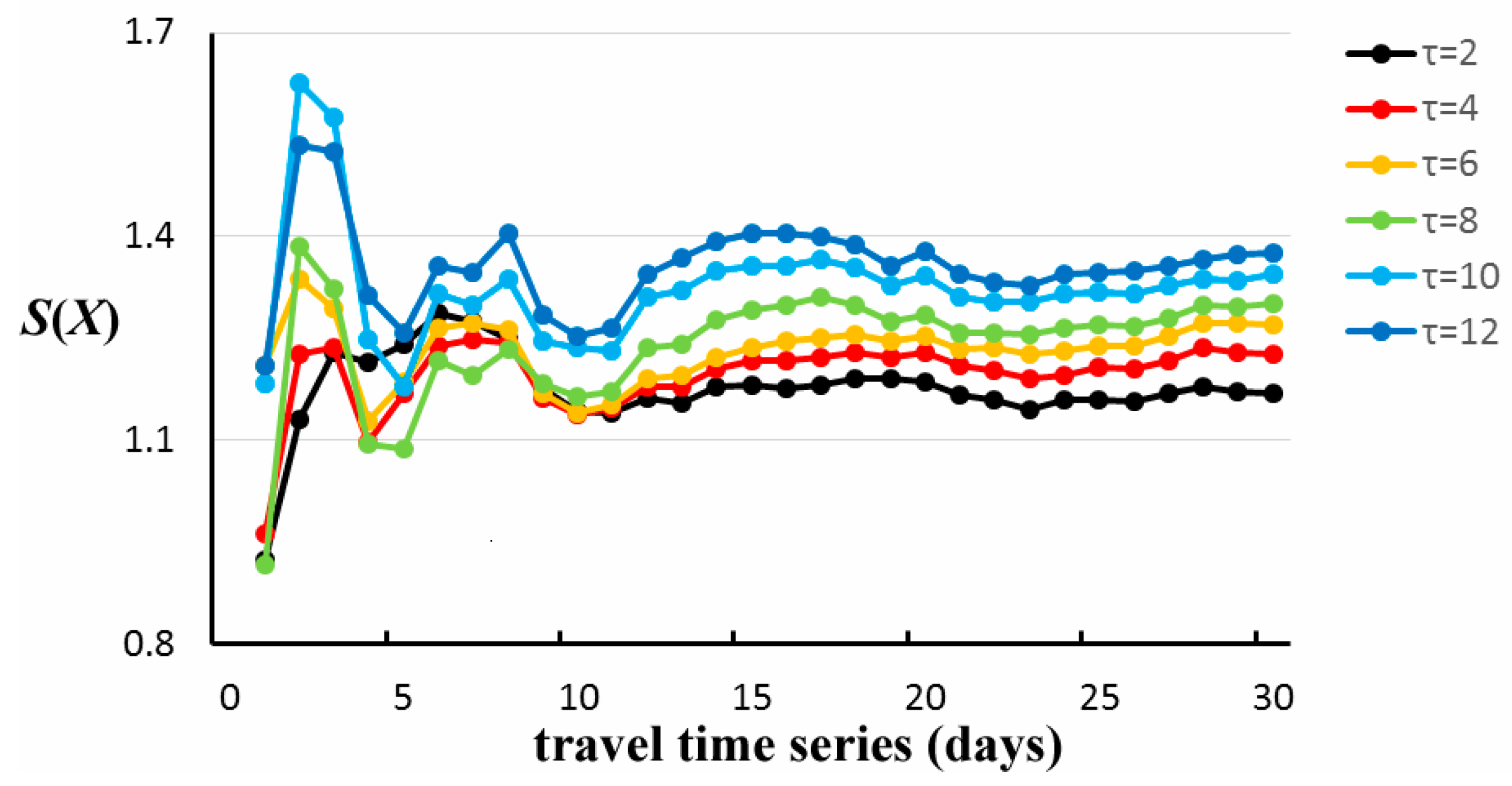
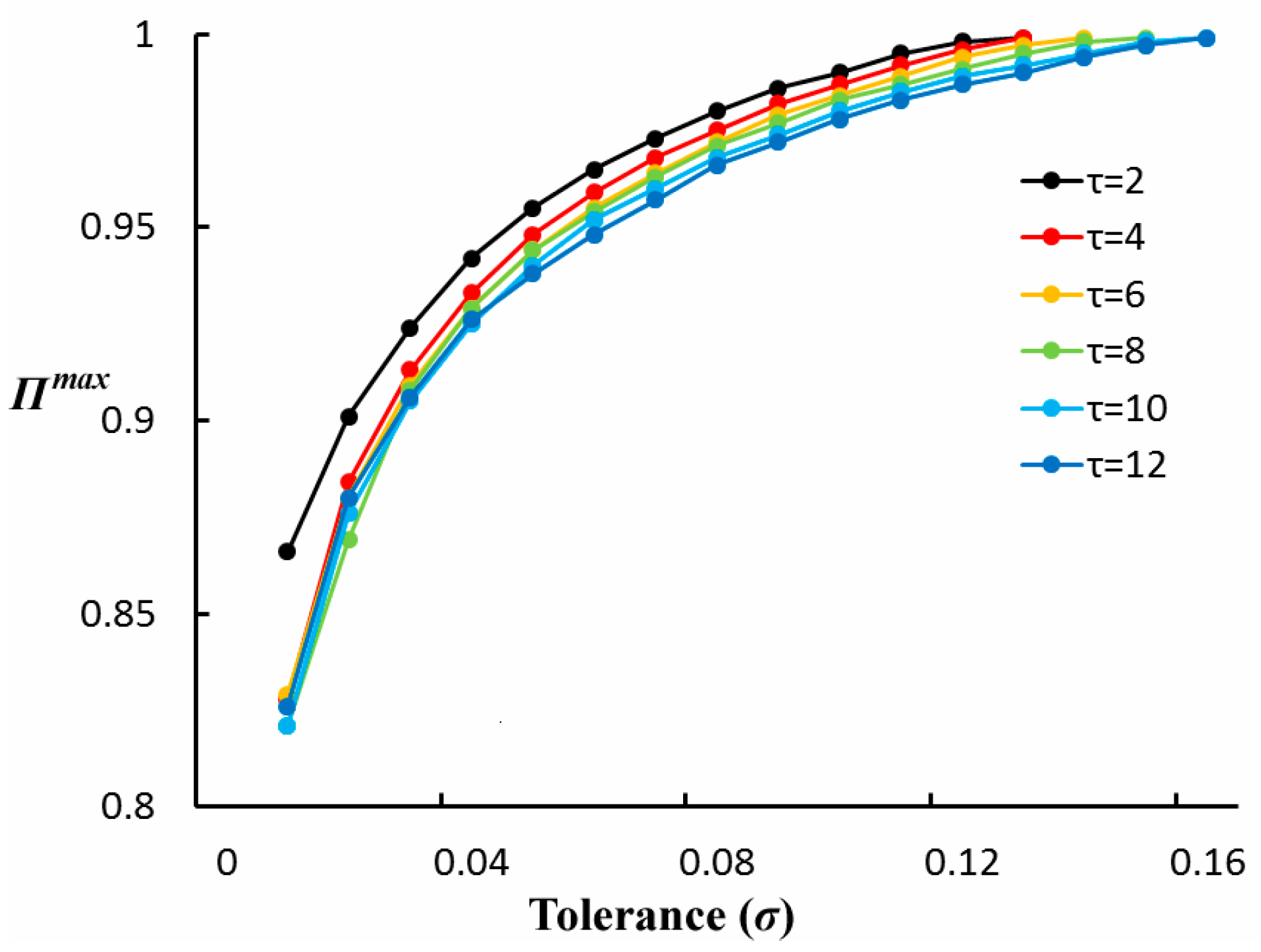
Figure 7 shows
of the 5 min travel time series with six time scales. There is a negative correlation between
and S(X). The higher the
is and the lower the S(X) is in shorter time scales, i.e.,
= 2, the lower the
is and the higher the S(X) is in longer time scales. At the same tolerance level, travel time series with a lower
value are easier to predict than those with a higher
. With the expansion of
,
gradually increases to 0.999.
is limited by
. Obviously, the higher
is, the higher the tolerance is to predictive error, the greater the
is, and the more accurate the prediction is.
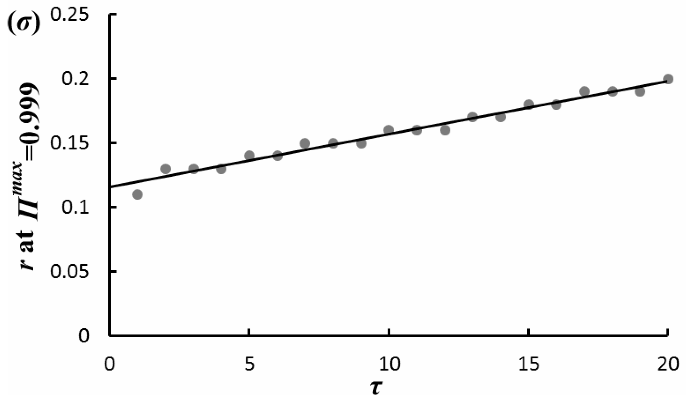
For the possibility of perfect theoretical prediction,
Figure 8 shows the tolerance of perfect prediction in multiple time scales. The ranges of
are from 1 to 20. Black line represents the trends of
with a
of 0.999. For example, the next travel time in
can be accurately predicted with
by the appropriate prediction model. The growth trend of
indicates that a higher
is more difficult to predict, and their perfect prediction needs greater tolerance ranges.
3.3.3. Series Length
Next, we analyze the influence of series length on entropy and predictability.
Figure 9 shows the entropy of travel time series in six time scales with different series length. The series length of a one-day 5 min travel time series is 288, and so on. Meanwhile,
, and
. It can be seen that these higher entropy are in 2 day or 3 day travel time series, and the more stable trends are in the >14 day (i.e., two weeks) travel time series. We can think that entropy of a >14 day travel time series is roughly independent of series length.
Table 1 shows that the statistics of entropy to support these findings, where
is the average value of entropy of all travel time series, and
is the standard deviation of all entropy. The
of >14 days is much lower than those of <14 days, and the most stable series is the >14 day travel time series with
and
. Therefore, we can demonstrate that the complexity of the >14 day travel time series is stable and is independent of series length.
Similarly,
Figure 10 demonstrates the smallest value of predictability of 2 day or 3 day travel time series and the stationarity and independence of predictability of the >14 day travel time series. In
Table 1,
denotes the average value of travel time predictability, and
denotes the standard deviation of travel time predictability. Great differences between the
of the >14 day travel time series and the <14 day travel time series present the stable predictability of the >14 day travel time series. In addition, we can demonstrate that the most stable predictability is in the >14 day travel time series with
and
.
3.3.4. The Validity of Travel Time Predictability
To validate the travel time predictability, two prediction models, i.e., AutoRegressive Integrated Moving Average (
ARIMA) [
35], and Back Propagation Neuro Networks (
BPNN) [
36], are employed to predict future travel time.
The ARIMA model is a method for time series analysis and prediction. Since travel time series have obvious fluctuation differences between weekdays and weekends, we use the seasonal ARIMA (SARIMA) model, denoted , to predict future travel time, where is the order of the autoregressive (AR) part, is the order of the moving average (MA) part, is the degree of difference for reducing the non-stationarity of time series, is the number of periods per season, and , , refer to the AR, differencing, and MA terms for the seasonal part of the ARIMA model. Due to the stationary and weekly change period of travel time series in our experiments, we set , , and . By testing the autocorrelation function (ACF) and the partial autocorrelation function (PACF) of complete and seasonal part travel time series, we set , , , and . Then, we use to predict future travel time in the selected route.
As a neuro network method, the BPNN model includes an input layer, a hidden layer, and an output layer. It can learn and store large amounts of input–output mapping by model training to represent and predict the dynamic and non-linear processes. In our experiments, the BPNN model has three inputs, i.e., the date, the time of day, and the day of week, and one output, i.e., the travel time, the number of nodes in the hidden layer is 7, the learning rate () is 0.9, and the momentum factor () is 0.7.
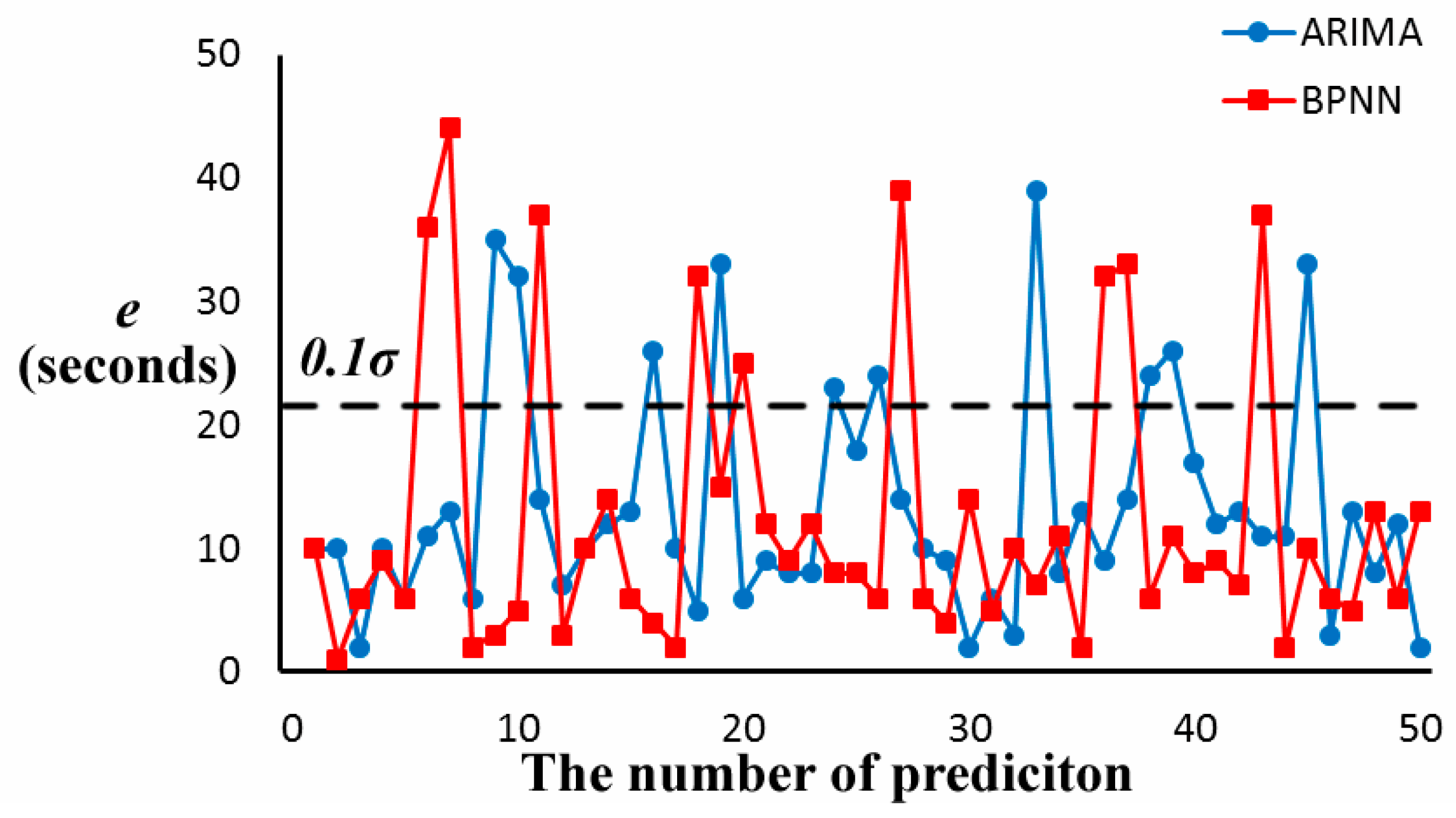
Figure 11 shows the errors of travel time prediction with
ARIMA and
BPNN models in 5 min travel time series. We set
(about 22 s),
, and
. We predict 50 times with
ARIMA and
BPNN, respectively, and let
be the absolute value of the difference between predictive value and actual value. The dashed line indicates the tolerance
. It can be seen that most dots are below it. The statistical results of travel time prediction of the 5 min travel time series are shown in
Table 2.
denotes the average predictability of 50 predictions in the 5 min travel time series. If
is less than
(below the dashed line of
Figure 11), it is a successful prediction. The number of successful predictions is 40 with
ARIMA, and 41 with
BPNN. Compared with
of 0.952, the success rates of prediction are lower, while their average errors, 13.46 and 12.42, are lower than tolerance
, 22.
To comprehensively evaluate the relationships between travel time predictability and prediction results, two group comparisons were conducted.
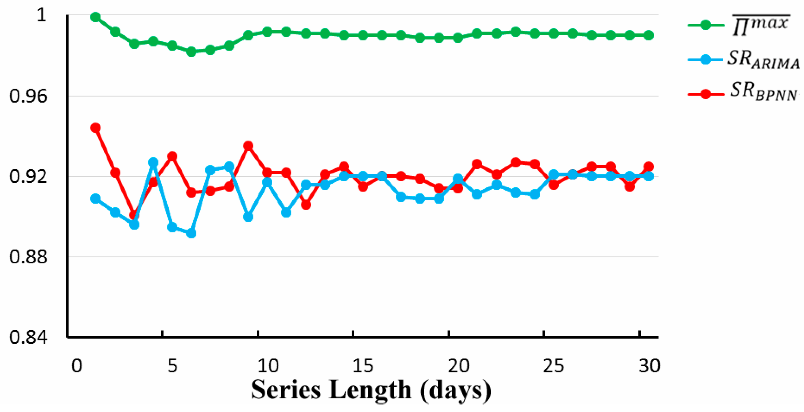
Figure 12 shows the comparison results between travel time predictability and prediction results in the 5 min travel time series with different series lengths of 1–30 days. The average prediction results of 100 experiments of each travel time series are presented:
,
, and
. Let
be the success rate of travel time prediction by
ARIMA, and let
be the success rate by
BPNN. There is a significant statistical difference between
(or
) and
. It indicates that the actual performance (
and
) of
ARIMA and
BPNN lags far behind the theoretical optimal value of success rate of travel time prediction, and the performance of travel time prediction is still great room for improvement. Note that the change trends of
or
are basically consistent, as shown in
Table 3, with the standard deviation (
) of the travel time predictability, and the predicted results of
ARIMA and
BPNN with shorter, 14-day series lengths have obvious higher values than the longer, 14-day series length, which indicates that the accuracy of prediction is affected by the complexity of the travel time series and demonstrates the validity of travel time predictability.
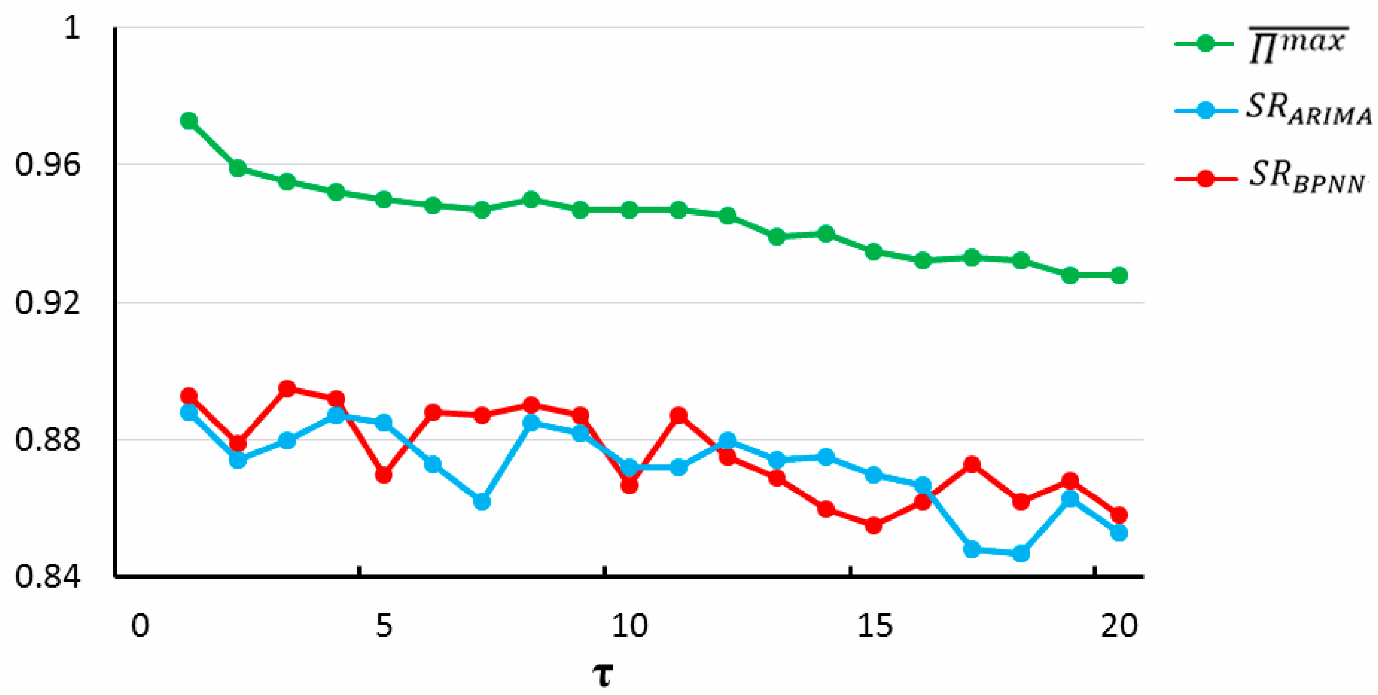
The same situation occurs in
Figure 13. We compare
and the prediction results in different time scales of 1–20 with
, and
. With the increase of time scales, travel time predictability and the success rates of two prediction models decline synchronously.
The proposed travel time predictability is a valid measurement of travel time series for correct prediction, which provides an achievable target to the development of travel time prediction methods and contribute to a differentiated scheme of travel time prediction.
4. Discussion and Conclusions
This paper defines travel time predictability as the probability of correctly predicting future travel times based upon historical travel time series and develops an entropy-based approach to measure the upper bound of travel time predictability. Multiscale entropy of travel time series is calculated to evaluate its complexity. The upper bound of travel time predictability is found to be related to entropy. Travel time predictability expresses the characteristics of travel time series itself and is an expected value of data-based prediction performance.
A case study in an express section road in Shanghai, China is designed. The data source is a large amount of taxi cab trajectory data collected in April 2015. By analyzing the effectiveness of the time scales and tolerance to entropy and travel time predictability, we demonstrate that time scales and tolerance are positively related to the entropy and negative related to travel time predictability. In addition, we reveal the higher value of entropy and the lower predictability of 2 day or 3 day travel time series and the more stable values of >14 day travel time series. Finally, two prediction models, ARIMA and BPNN, are employed to predict travel time based on historical travel time series and to examine the validity and reliability of travel time predictability. Though travel time predictability is independent of the prediction method, it can aid the development of travel time prediction methods and contribute to a differentiated scheme for travel time prediction in diverse traffic environment.
Future efforts may be pursued in two directions. First, the comprehensive investigation and verification of travel time predictability should begin in a larger network with multiple data sources to show the capability of capturing the entropy, which contributes to deeper traffic knowledge discovery and differentiation traffic police formulation. Second, the scope of predictability should be extended and the possibility of applying predictability to other types of time series may be surveyed.


