
Minimum Entropy Active Fault Tolerant Control of the Non-Gaussian Stochastic Distribution System Subjected to Mean Constraint

School of Electrical Engineering, Zhengzhou University, Zhengzhou 450001, China
*
Author to whom correspondence should be addressed.
Entropy 2017, 19(5), 218; https://doi.org/10.3390/e19050218
Submission received: 23 March 2017
/
Revised: 24 April 2017
/
Accepted: 3 May 2017
/
Published: 11 May 2017
Abstract
:Stochastic distribution control (SDC) systems are a group of systems where the outputs considered is the measured probability density function (PDF) of the system output whilst subjected to a normal crisp input. The purpose of the active fault tolerant control of such systems is to use the fault estimation information and other measured information to make the output PDF still track the given distribution when the objective PDF is known. However, if the target PDF is unavailable, the PDF tracking operation will be impossible. Minimum entropy control of the system output can be considered as an alternative strategy. The mean represents the center location of the stochastic variable, and it is reasonable that the minimum entropy fault tolerant controller can be designed subjected to mean constraint. In this paper, using the rational square-root B-spline model for the shape control of the system output probability density function (PDF), a nonlinear adaptive observer based fault diagnosis algorithm is proposed to diagnose the fault. Through the controller reconfiguration, the system entropy subjected to mean restriction can still be minimized when fault occurs. An illustrative example is utilized to demonstrate the use of the minimum entropy fault tolerant control algorithms.
1. Introduction
Fault diagnosis (FD) and fault-tolerant control (FTC) has long been regarded as an important and integrated part in control systems. The research of this aspect has been carried out for nearly thirty years, where the major research is aimed at deterministic systems. However, most practical systems are subjected to random inputs from sensor noises [1], random disturbances [2] or random parameter changes. In order to improve the reliability of the control system, the research of fault diagnosis and fault-tolerant control for stochastic dynamic systems has been one of the liveliest research areas in control theory and practice [3]. For stochastic systems, the so-far obtained FDD (fault detection and diagnosis) approaches can be classified as
Moreover, in a safety-critical system, the role of a fault-tolerant control system is extremely important. One of its functions is to steer the process to a safe state whenever undesirable events occur. A fault-tolerant controller can be able to attenuate the effects caused by random variables.
For most control algorithms, it is supposed that system noise obeys Gaussian distribution. Traditional statistics such as mean and variance can be used to represent the randomness of the system output. However, for non-Gaussian systems, the variance cannot fully represent the randomness of the system output. A more general measure, rather than just the variance of the system output, needs to be considered for the randomness of the system output of non-Gaussian stochastic systems. Therefore, entropy concept [7] is proposed to measure the uncertainty of the system output of stochastic systems.
In existing FTC results of SDC systems, it is assumed that the target PDF is pre-specified. Nonlinear filters are designed to detect and diagnose the fault of the stochastic distribution system based on square-root approximation [8]. However, fault tolerant control is not considered. A nonlinear adaptive observer-based fault diagnosis algorithm is proposed to diagnose the fault in the dynamic part of the non-Gaussian SDC systems based on the rational square-root B-spline approximation model [9]. Through the controller reconfiguration, a good output PDF tracking can still be realized when fault occurs. An iterative learning observer based fault estimation algorithm is proposed [10] and the fault tolerant controller is designed so as to make the post-fault PDF still track the given distribution. However, in most cases, the objective PDF can’t be determined in advance and, as a result, the reasonable fault tolerant tracking controller cannot be designed. Therefore, minimum entropy control of the system output can be considered as an alternative strategy. A minimum entropy control method of closed-loop tracking errors is proposed [11]. A nonlinear observer is designed to obtain the pseudo-weights vector [12]. Then, the PDF tracking control and the minimum entropy control are developed. An integrated design of fault diagnosis and fault tolerant control (FTC) for nonlinear systems using Takagi–Sugeno (T–S) fuzzy models is proposed in [13]; meanwhile in the presence of the model uncertainty along with actuator/sensor faults and external disturbance. An augmented state unknown input observer is proposed to estimate the fault and the system state simultaneously, and using the fault estimation information, an FTC controller is developed to ensure the robust stability of the closed-loop system. The design scheme of thruster failure tolerant control for underwater vehicles is proposed [14], where each thruster of the underwater vehicle can rotate, offering a significant advantage to optimize its control. Active and passive fault-tolerant control systems (FTCSs) aer demystified by examining the similarities and differences between these two approaches from both philosophical and practical points of view in [15]. A new method is proposed [16] to minimize the closed loop randomness for general dynamic stochastic systems using the entropy concept. However, a fault item is not involved in this literature. This forms the point of this paper, where the entropy concept is used for design of the required fault tolerant controllers of stochastic systems.
In this paper, the rational square-root B-spline model [17] is used to represent the dynamics between the output PDF and input. The considered system in [17] is subjected to any arbitrary bounded random input and the purpose of the control input design is to make the output probability density function of the system output track a given distribution function as close as possible, that different from the objective PDF known in literature [17], the target PDF in this paper can not be determined in advance. Considering the existence of the fault, a nonlinear adaptive observer based fault diagnosis algorithm is proposed to diagnose the fault. Through the controller reconfiguration, the system entropy can still be minimized when fault occurs. The contribution of this paper is that the entropy concept is introduced to design of fault tolerant control for non-Gaussian stochastic distribution systems when the objective PDF can not be determined in advance.
The rest of this paper is organized as follows. Section 2 presents the model description, where a nonlinear dynamic relationship is considered. An observer is constructed in Section 3 for fault detection. In Section 4, the nonlinear adaptive observer based fault diagnosis algorithm is proposed, and the rational square-root B-spline model, which is different from that in [10], is used for the shape control of the system output PDF. Section 5 gives the design process of fault tolerant control. Simulation results of FD and FTC are presented in Section 6, followed by some concluding remarks in Section 7.
2. Model Description
Denote as a uniformly bounded stochastic process variable and assume that it represents the output of a stochastic system at sample time t. Denote as the control input that controls the distribution of . At any time, can be characterized by its probability density function , which is defined by
where represents the probability of the output lying inside the interval when is applied to the system. It also means that the shape of the output probability density function, is controlled by a crisp input . It is assumed that interval is known and the output probability density functions is continuous and bounded. Using the rational square-root B-spline function approximation principle [17], the rational square-root B-spline expansion as follows,
where are the pre-specified basis functions defined on and are the corresponding weights.
For most systems, a dynamic relationship between and u is expressed. In this paper, a nonlinear dynamic relationship will be considered. This leads to the following model for the considered dynamic stochastic system:
where is the state vector, is the output weight vector, is the control input vector and is the fault vector. , , , , and are system parameter matrices. Equation (2) represents the dynamic model of the weights vector. Equation (3) describes the static output PDF model using the rational square-root B-spline expression, where
Assumption A1.
The nonlinear function should satisfy the following Lipschitz condition:
where is a Lipschitz constant.
3. Fault Detection
The purpose of the fault detection is to use input vector in Equation (2) and output probability density function to detect the fault F. In order to detect such a fault, an observer is constructed [18] as follows:
where is the estimated state, is the residual signal, is the pre-specified weighting vector defined on and K is the gain of the observer.
Denote the observation error vector as
The residual signal can be calculated as follows:
where .
Assume that the basis function and are selected such that the pair is observable. The gain can be selected such that matrix is .
Lemma 1.
There exists a (, , ) such that the following equation
holds.
Theorem 1.
It is supposed that there exist two positive definite matrices P and Q such that the following equalities
hold, and then the observation error system is asymptotically stable.
Proof.
When no fault occurs, . Denote , and is the gain matrix of the observer. Then, the error dynamic system can be further formulated as
The Lyapunov function is selected as follows:
It can be shown that
when
hold, and then . The proof is completed. ☐
The fault can be detected when , where is a pre-specified threshold.
4. Fault Diagnosis Algorithm
Once the fault has been detected, the fault diagnosis needs to be carried out in order to estimate the size of the fault. A fault diagnosis observer is constructed [19] as follows:
where is the estimation of F. It is assumed that , , and then
Denote , and the gain can be selected such that matrix is . Then, the error dynamic system can be obtained as follows:
Assumption A2.
Suppose that , where N is a positive constant.
Theorem 2.
It is supposed that there exist constant and two positive definite matrices , such that the following equality holds:
and the adaptive tuning law is selected as follows:
and then the error dynamic system (14) is stable.
Proof.
The Lyapunov function is selected as follows:
and then the first derivative of is formulated as follows:
where
From Assumption 2 and Theorem 2, it can be obtained that
When , it can be obtained that . This means that when fault occurs in system (2), the observation error system is stable. ☐
5. Fault Tolerant Control
Once the fault has been diagnosed, the controller that is designed for the healthy system should be modified so as to compensate for the performance losses caused by the fault in the system.
When the objective PDF can not be determined in advance, or no objective PDF can be used, control target of the SDC system can be translated into controlling the entropy of the system output. It has been pointed out that the entropy has been used to characterize the uncertainty of the output variables for non-Gaussian stochastic systems. Thus, the uncertainty is expected to be as small as possible.
When the position of the output variable’s PDF is not determined, the minimum entropy of the output variables is generally difficult to be determined in practice. Therefore, control target subjected to mean constraint will be suitable for the solution of the minimum entropy controller.
Since the mean and entropy of a non-Gaussian stochastic variable are independent of each other, these two terms may be addressed separately. For this purpose, the following performance function is used
It can be seen that the first term in Equation (20) is the error between the mean and its target value , where . The second term is the Shannon entropy of the output variables, and the third term is a natural quadratic constraint for the control input, where .
The purpose of the controller design is to find the required optimal control input such that the performance index function is minimized. This purpose can be realized by selecting a control input such that the performance function does not increase. The performance index of the close-loop system can be seen as a Lyapunov function. In order to minimize J in Equation (20), the first order derivative of J can be readily formulated that
At this stage, by selecting the following control input
where , it can then be formulated that
Therefore, the performance index is convergent.
From Equation (2), it can be obtained that
When no fault occurs, , using Equation (24), it can be obtained that
When the fault occurs and has been diagnosed, it can then be rewritten as
where is the reconfigured controller. The state x and fault F can be substituted by the state of the fault diagnosis observer state and the fault estimation , respectively.
6. Simulation Example
The following B-spline is selected as
where
.
It is assumed that the system dynamics can be represented as
where ,
Positive definite matrices and are selected as follows:
It can be solved via linear matrix inequality (LMI) related to Equations (9) and (15) to obtain the detect observer gain diagnostic observer gain and the parameters of fault estimation adaptive tuning rule .
To simulate the algorithm, it is assumed that the three types of faults are constructed as follows:
The step fault:
The intermittent fault:
The incipient fault:
The ramp-like fault:
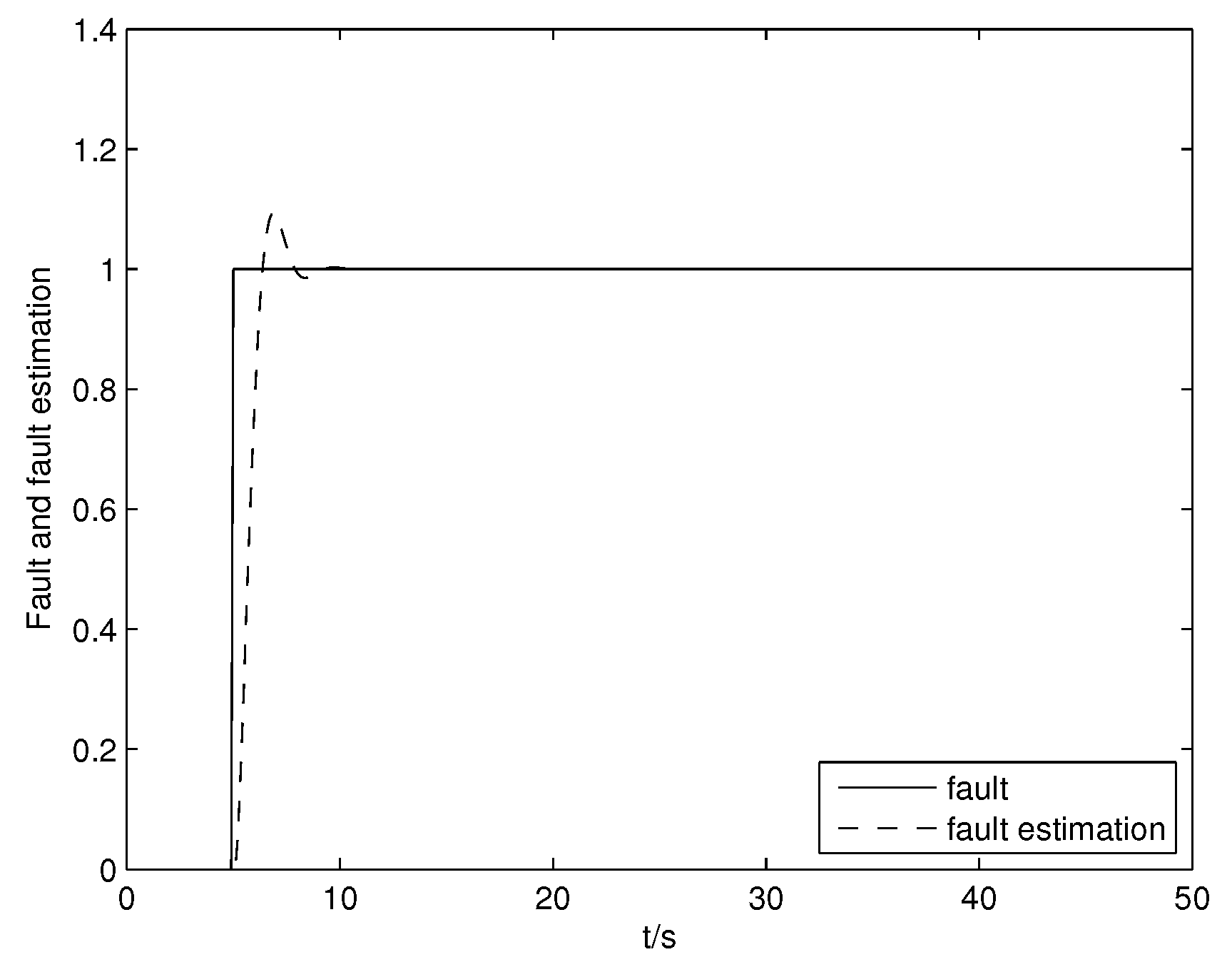
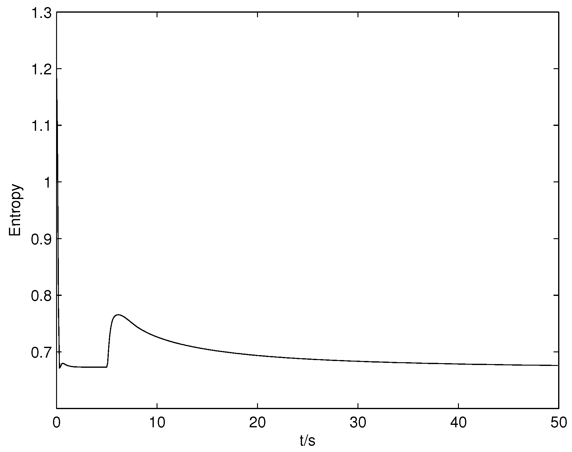
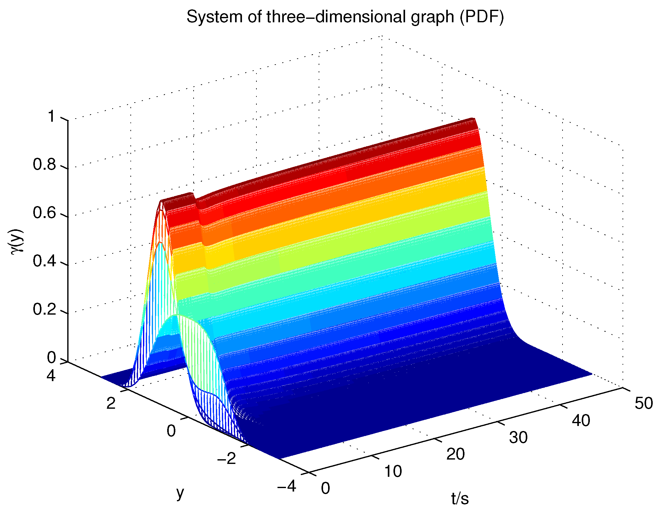
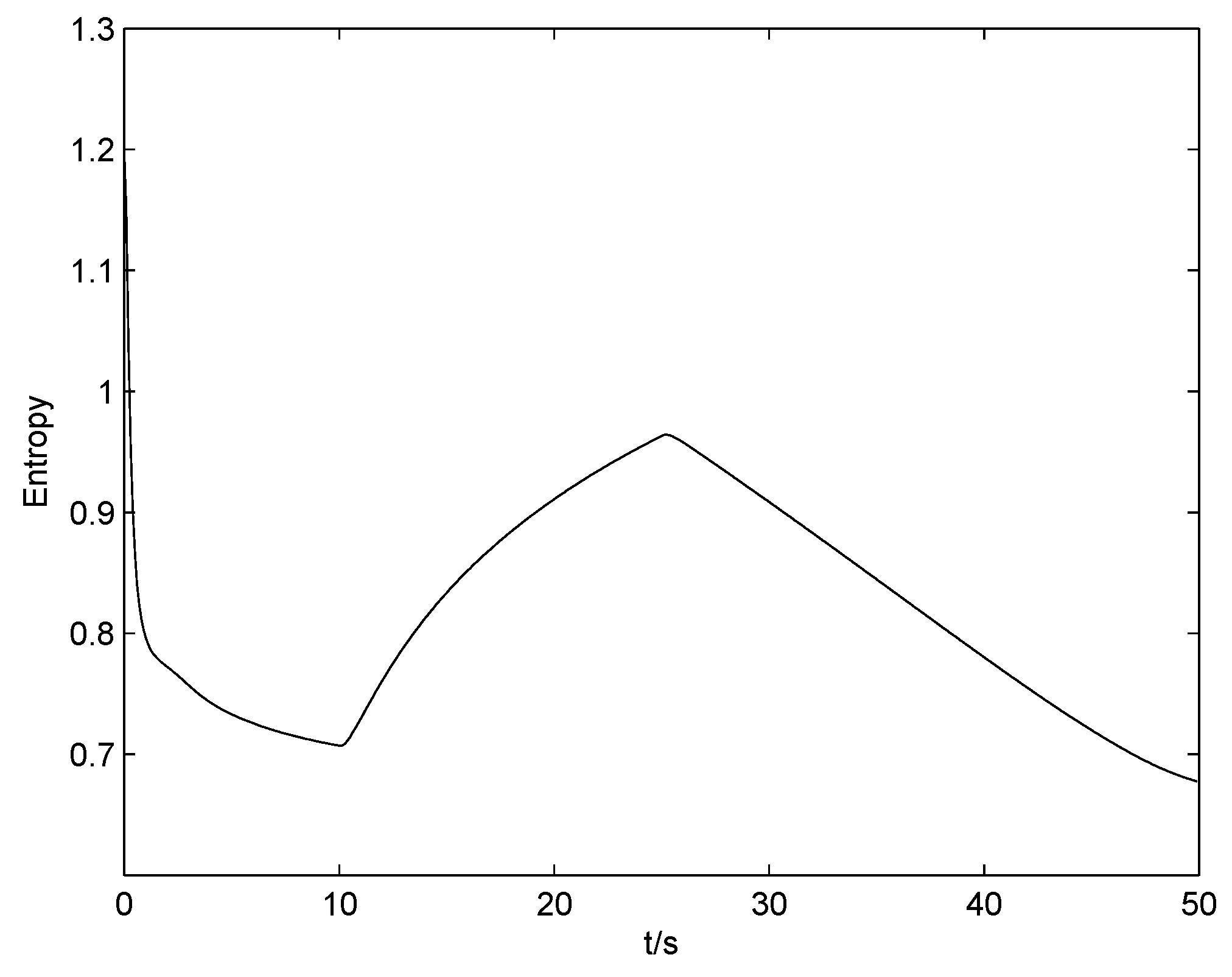
Case 1: When a step fault occurs, the fault detection signal is shown in Figure 1 and the fault diagnosis result is shown in Figure 2. From the two figures, it can be concluded that desired fault detection and diagnosis results have been obtained. If the system works normally, then we have . Figure 3 shows the result of the output entropy and Figure 4 shows the result of the output PDF. Figure 5 presents the response of the mean. In the simulation, fault is set to 1 after 5 s. Figure 6 shows the changes of the entropy when a fault has occurred in the system. It can be seen that the control input is driving the system towards the direction of less randomness. From Figure 7, it can be seen that the post-fault PDF can still follow the faultless PDF, leading to good fault tolerant control results. Figure 8 presents the response of the mean when a fault has occurred in the system, and it can be seen that the mean value levels off and approaches the objective value.
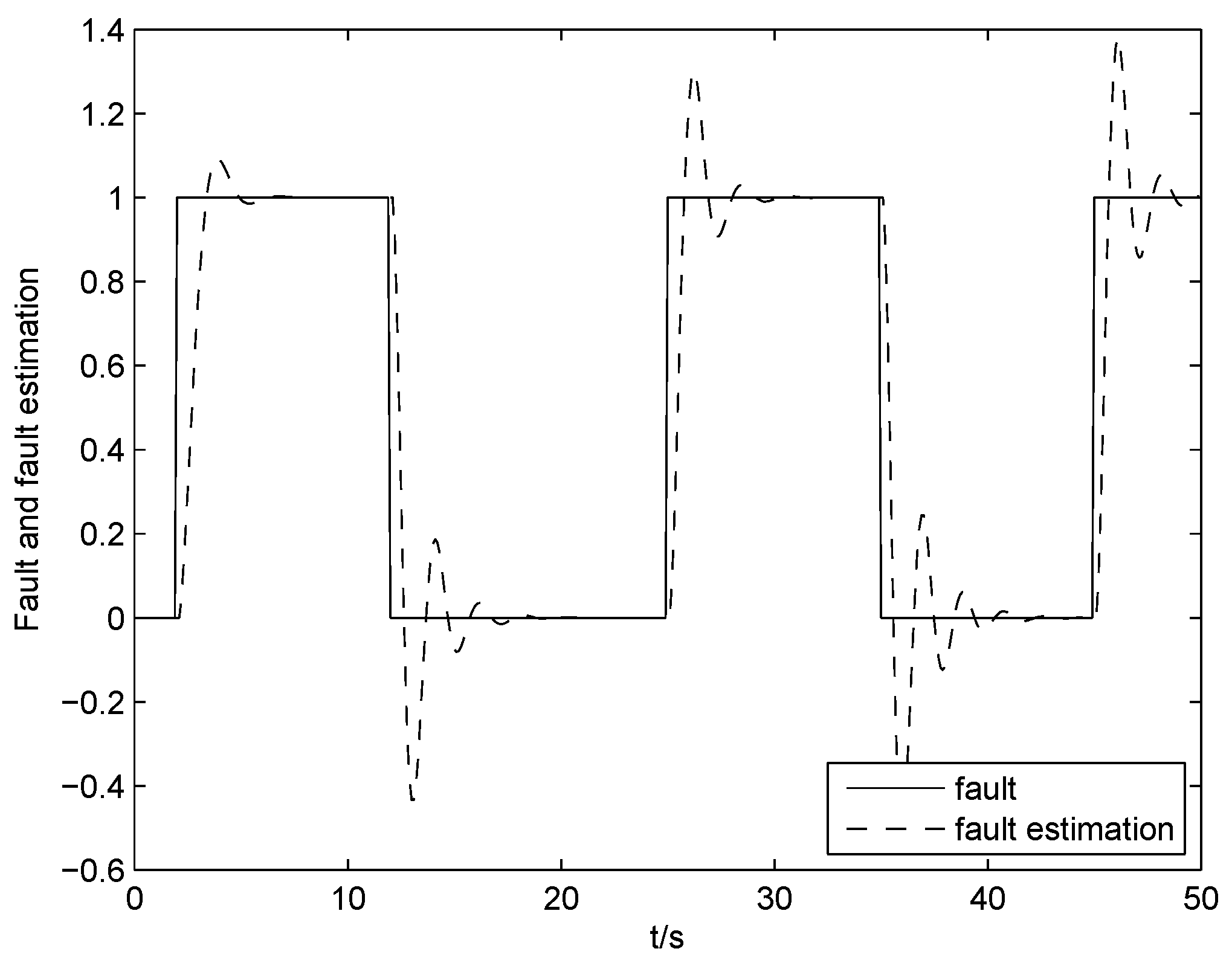
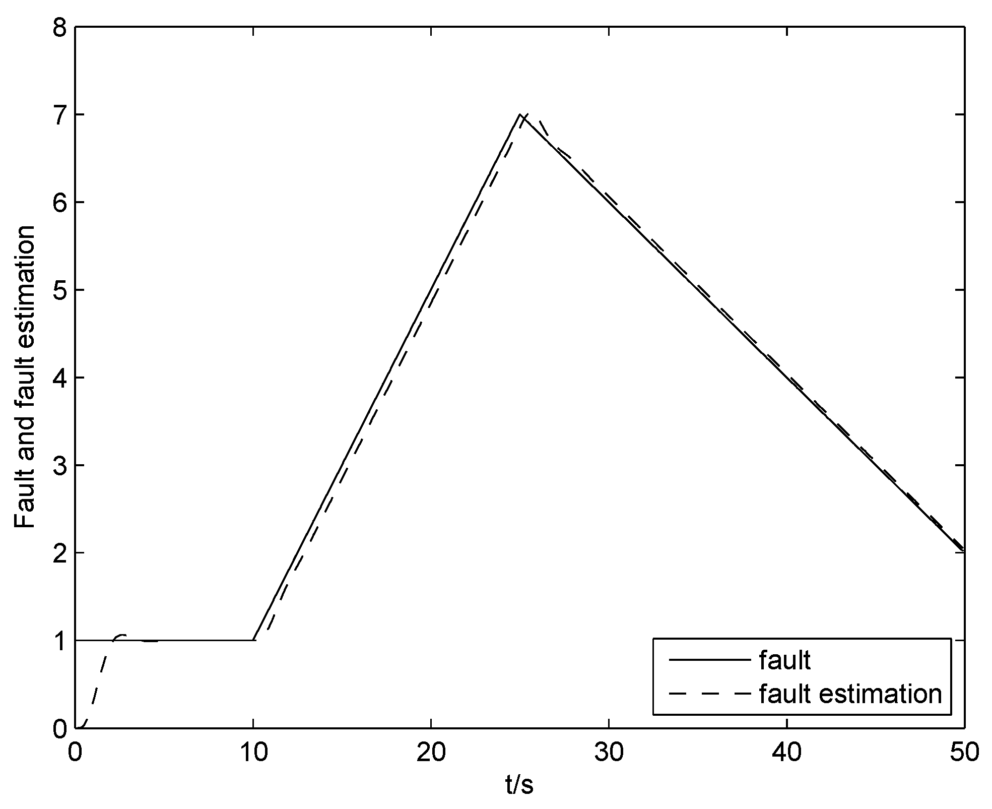
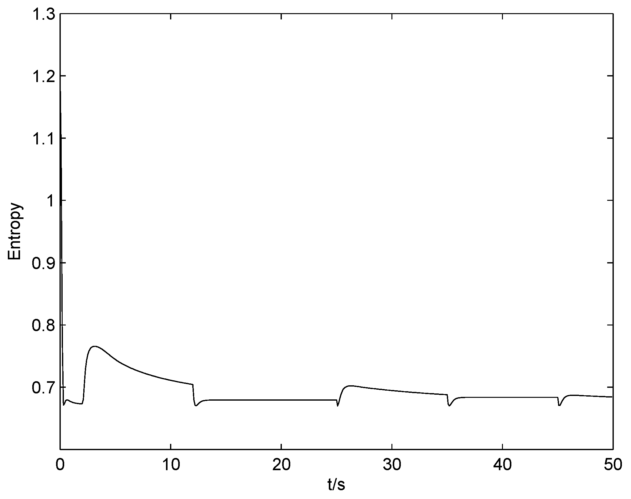
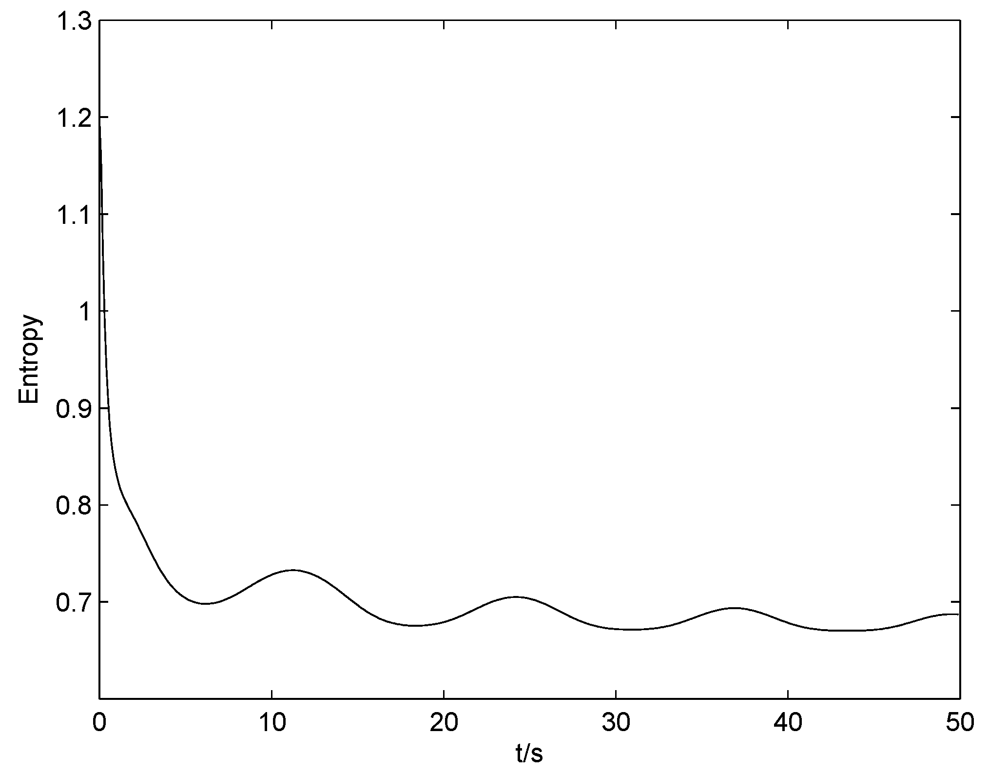
Case 2: When the intermittent fault, incipient fault and ramp-like fault occur, the fault diagnosis results are shown in Figure 9, Figure 10 and Figure 11. From the three figures, it can be concluded that diagnosis results have been obtained. Figure 12, Figure 13 and Figure 14 show the change of the entropy when the three faults have occurred in the system. It can be seen that the control input is driving the system towards the direction of less randomness.
7. Concluding Remarks
In this paper, when objective PDFs can not be determined in advance, the entropy concept is applied to the design of a fault tolerant controller for a non-Gaussian stochastic distribution system. The mean represents the center location of the stochastic variable, and it is reasonable that a minimum entropy fault tolerant controller can be designed under the restriction of the mean. A rational square-root B-spline function approximation model and the nonlinear dynamic system have been used to formulate the stochastic distribution system. A performance function that includes the entropy term and a mean constraint term is used to design the fault tolerant controller. The performance index is regarded as a Lyapunov function. Using the Lyapunov stability criterion, the stability of the whole system can be guaranteed. Furthermore, through the controller reconfiguration, the system entropy can still be minimized. The simulations have further confirmed the proposed fault diagnosis and fault tolerant control results.
Acknowledgments
This work is supported by the National Natural Science Foundation of China (NSFC) under Grant 61374128, the Science and Technology Innovation Talents 14HASTIT040 in Colleges and Universities in Henan Province, China, and the Open Project of the Chinese State Key Laboratory of Synthetical Automation for Process Industries.
Author Contributions
Haokun Jin, Yacun Guan and Lina Yao conceived and designed the experiments; Haokun Jin and Yacun Guan performed the experiments; Haokun Jin analyzed the data; Lina Yao contributed analysis tools; Haokun Jin and Yacun Guan wrote the paper.
Conflicts of Interest
The authors declare no conflict of interest.
References
- Juricic, D.; Zele, M. Robust detection of sensor faults by means of a statistical test. Automatica 2002, 38, 737–742. [Google Scholar] [CrossRef]
- Guo, L.; Wang, H. Bibliographical review on reconfigurable fault-tolerant control systems. Annu. Rev. Control 2006, 51, 695–700. [Google Scholar]
- Wang, H. Bounded Dynamic Stochastic Systems: Modelling and Control; Springer: London, UK, 2000. [Google Scholar]
- Isermann, R. Model-based fault-detection and diagnosis-status and applications. Annu. Rev. Control 2005, 29, 71–85. [Google Scholar] [CrossRef]
- Frank, P.M.; Ding, X. Survey of robust residual generation and evaluation methods in observer-based fault detection systems. J. Process Control 1997, 7, 403–424. [Google Scholar] [CrossRef]
- Li, P.; Kadirkamanathan, V. Fault detection and isolation in nonlinear stochastic systems a combined adaptive Monte Carlo filtering and likelihood ratio approach. Int. J. Control 2004, 77, 1101–1104. [Google Scholar] [CrossRef]
- Chen, R.H.; Mingori, D.L.; Speye, J.L. Optimal stochastic fault detection filter. Automatica 2003, 39, 377–390. [Google Scholar] [CrossRef]
- Guo, L.; Wang, H. Fault detection and diagnosis for general stochastic systems using B-spline expansions and nonlinear filter. IEEE Trans. Circuits Syst. I 2005, 52, 1644–1652. [Google Scholar]
- Yao, L.N.; Wang, A.P.; Wang, H. Fault detection, diagnosis and tolerant control for non-Gaussian stochastic distribution systems using a rational square-root approximation model. Int. J. Model. Identif. Control 2008, 3, 162–172. [Google Scholar] [CrossRef]
- Yao, L.N.; Qin, J.F.; Wang, H.; Jiang, B. Design of new fault diagnosis and fault tolerant control scheme for non-Gaussian singular stochastic distribution systems. Automatica 2012, 48, 2305–2313. [Google Scholar] [CrossRef]
- Yue, H.; Wang, H. Minimum entropy control of closed-loop tracking errors for dynamic stochastic systems. IEEE Trans. Autom. Control 2003, 48, 118–122. [Google Scholar]
- Zhou, J.L.; Yue, H.; Wang, H. Shaping of output PDF based on the rational square-root B-spline model. Acta Autom. Sin. 2005, 31, 343–351. [Google Scholar]
- Lan, J.L.; Patton, R.J. Integrated design of fault-tolerant control for nonlinear systems based on fault estimation and T-S fuzzy modelling. IEEE Trans. Fuzzy Syst. 2016, 99. [Google Scholar] [CrossRef]
- Ciabattoni, L.; Fasano, A.; Ferracuti, F.; Freddi, A.; Longhi, S.; Monteriu, A. A thruster failure tolerant control scheme for underwater vehicles. In Proceedings of the 12th IEEE/ASME International Conference on Mechatronic and Embedded Systems and Applications (MESA), Auckland, New Zealand, 29–31 August 2016; pp. 1–6. [Google Scholar]
- Jiang, J.; Yu, X. Fault-tolerant control systems: A comparative study between active and passive approaches. Annu. Rev. Control 2012, 36, 60–72. [Google Scholar] [CrossRef]
- Wang, H. Minimum entropy control of non-Gaussian dynamic stochastic systems. IEEE Trans. Autom. Control 2002, 47, 398–403. [Google Scholar] [CrossRef]
- Wang, H.; Zhang, J.H. Bounded Stochastic distributions control for pseudo armax stochastic systems. IEEE Trans. Autom. Control 2001, 46, 486–490. [Google Scholar] [CrossRef]
- Yao, L.N.; Peng, B. Fault diagnosis and fault tolerant control for the non-Gaussian time-delayed stochastic distribution control system. In Proceedings of the American Control Conference (ACC), Washington, DC, USA, 17–19 June 2013; pp. 5409–5414. [Google Scholar]
- Yao, L.N.; Feng, L. Fault diagnosis and fault tolerant tracking control for the non-Gaussian singular time-delayed stochastic distribution system with PDF approximation error. Neurocomputing 2016, 175, 538–543. [Google Scholar] [CrossRef]
Figure 1.
Fault detection signal.
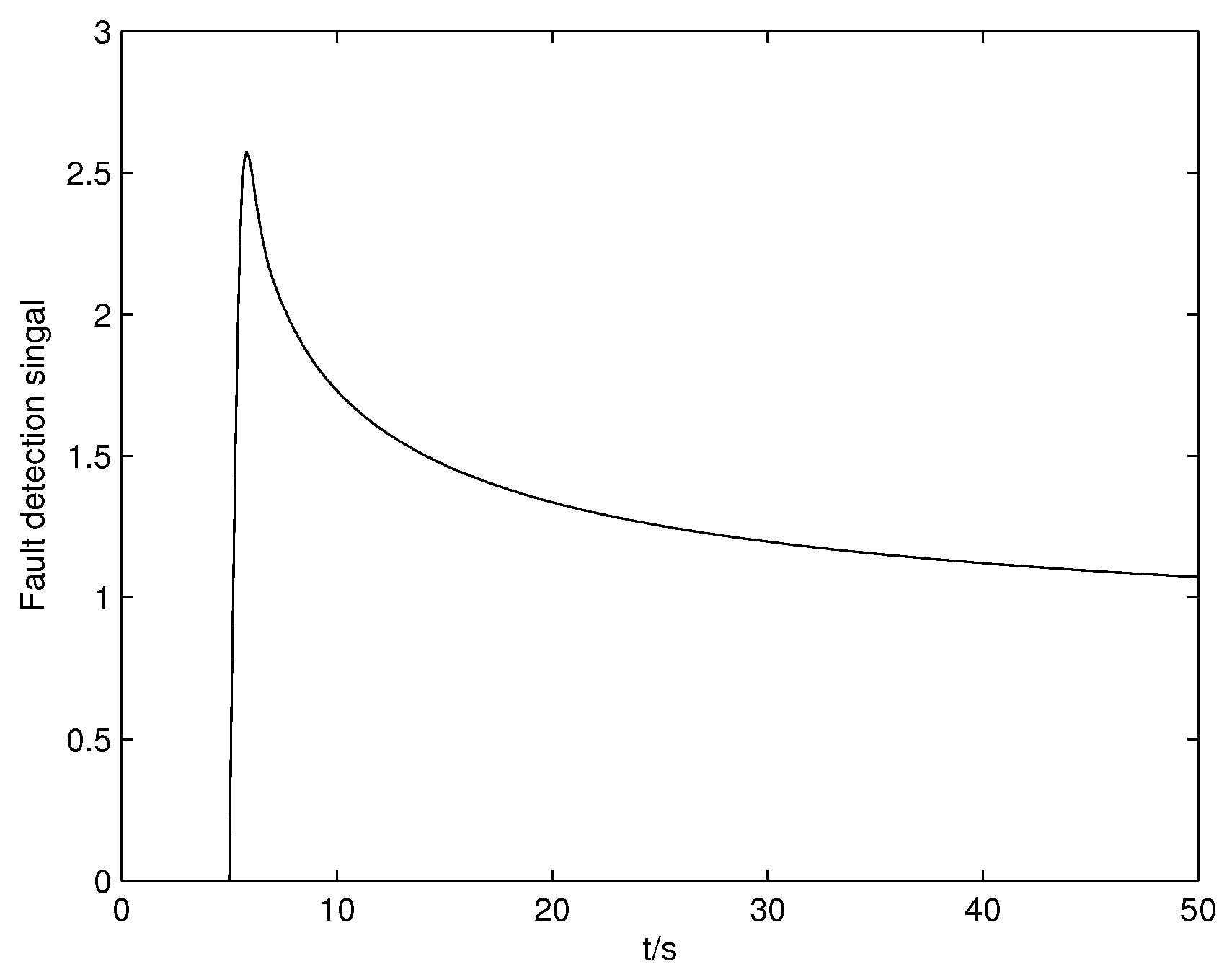
Figure 2.
The fault and fault estimation.

Figure 3.
The response of entropy when system is normal.
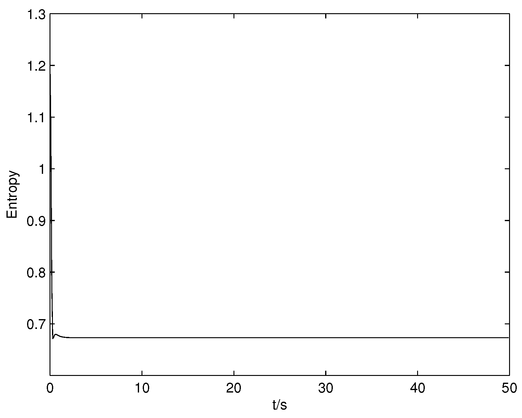
Figure 4.
The response of the output PDF when F = 0.

Figure 5.
The response of the mean when system is normal.
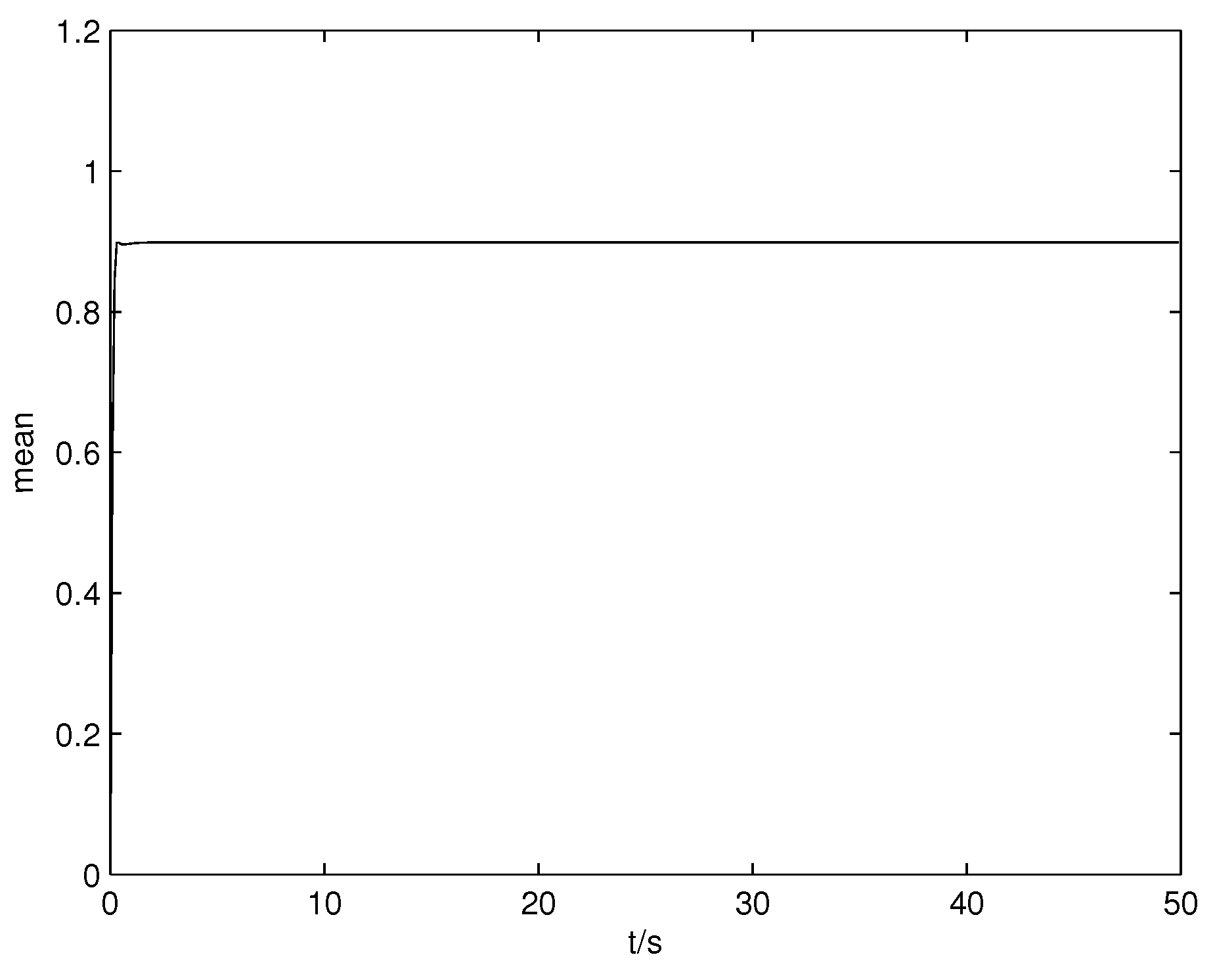
Figure 6.
The response of entropy after fault-tolerant control.

Figure 7.
The output PDF with fault-tolerant control.

Figure 8.
The response of the mean after fault-tolerant control.
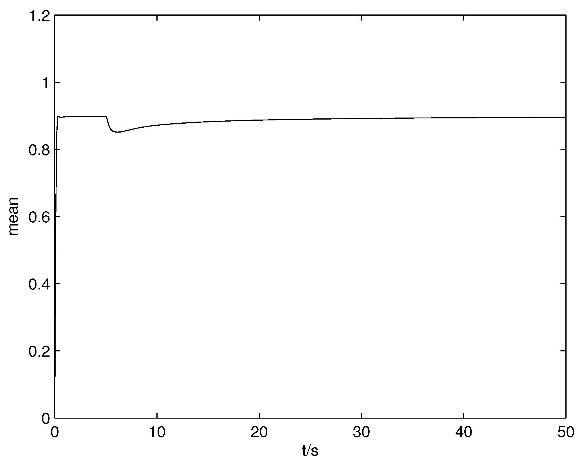
Figure 9.
The intermittent fault and fault estimation.

Figure 10.
The incipient fault and fault estimation.
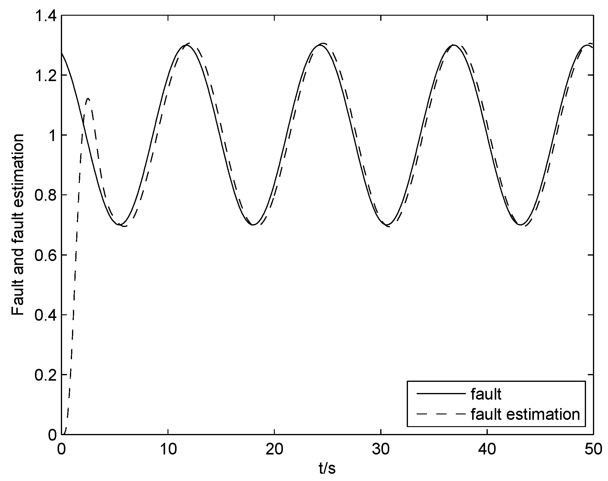
Figure 11.
The ramp-like fault and fault estimation.

Figure 12.
The response of entropy after fault-tolerant control for intermittent fault.

Figure 13.
The response of entropy after fault-tolerant control for incipient fault

Figure 14.
The response of entropy after fault-tolerant control for ramp-like fault.
© 2017 by the authors. Licensee MDPI, Basel, Switzerland. This article is an open access article distributed under the terms and conditions of the Creative Commons Attribution (CC BY) license (http://creativecommons.org/licenses/by/4.0/).
Share and Cite
MDPI and ACS Style
Jin, H.; Guan, Y.; Yao, L. Minimum Entropy Active Fault Tolerant Control of the Non-Gaussian Stochastic Distribution System Subjected to Mean Constraint. Entropy 2017, 19, 218. https://doi.org/10.3390/e19050218
AMA Style
Jin H, Guan Y, Yao L. Minimum Entropy Active Fault Tolerant Control of the Non-Gaussian Stochastic Distribution System Subjected to Mean Constraint. Entropy. 2017; 19(5):218. https://doi.org/10.3390/e19050218
Chicago/Turabian StyleJin, Haokun, Yacun Guan, and Lina Yao. 2017. "Minimum Entropy Active Fault Tolerant Control of the Non-Gaussian Stochastic Distribution System Subjected to Mean Constraint" Entropy 19, no. 5: 218. https://doi.org/10.3390/e19050218
Note that from the first issue of 2016, this journal uses article numbers instead of page numbers. See further details here.