
Information Entropy and Measures of Market Risk


Abstract
:1. Introduction
2. The Entropy of a Distribution Function and Measures of Market Risk and Uncertainty
2.1. The Entropy and Intraday Measures of Market Risk and Uncertainty
2.1.1. Entropy of a Distribution Function
- (i)
- F is right continuous;
- (ii)
- F is monotonically increasing;
- (iii)
- ;
- (iv)
- .
2.1.2. Empirical Distribution Function
- Step 1.
- Let be a fixed point and let be the bin width;
- Step 2.
- Define the bins as , obtaining a partition of the real line;
- Step 3.
- For , such as , let ;
- Step 4.
- The histogram estimator of the pdf is defined as ;
- Step 5.
- The empirical estimator of distribution function (CDF) is:
2.1.3. Kernel Density Estimator
2.1.4. Estimation of the Entropy of a Distribution Function
- Step 1.
- Estimate the distribution function, obtaining values for ;
- Step 2.
- Sample from the distribution function, using the sampled function for ;
- Step 3.
- Define a quantum ; then , if ;
- Step 4.
- Compute the probabilities ;
- Step 5.
- Estimate the entropy of the distribution function: .
2.1.5. Properties and Asymptotic Behaviour of the Entropy of a Distribution Function
2.1.6. Optimal Sampling Frequency
- (1)
- Intraday VaR at significance level α computed from observations at frequency ν, being the α-quantile of the distribution of intraday returns, so that the following is satisfied:
- (2)
- Intraday ES at significance level α computed from observations at frequency ν, defined as:
- (3)
- Intraday Realized Volatility computed from intraday returns at frequency ν, computed as:
2.1.7. Static Models
2.1.8. Dynamic Models
2.2. Quantile Regressions
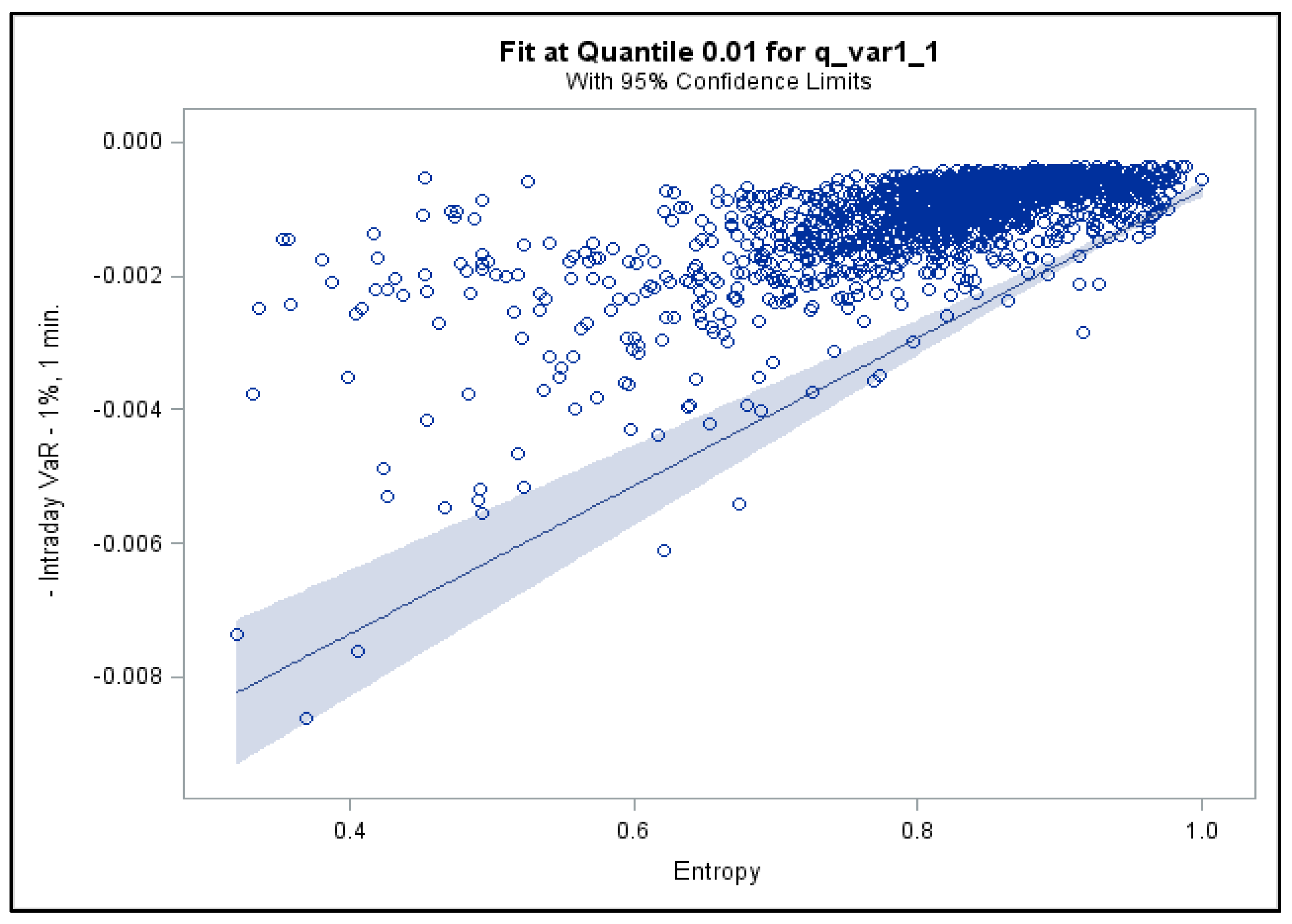
2.2.1. Quantile Regressions for Intraday VaR
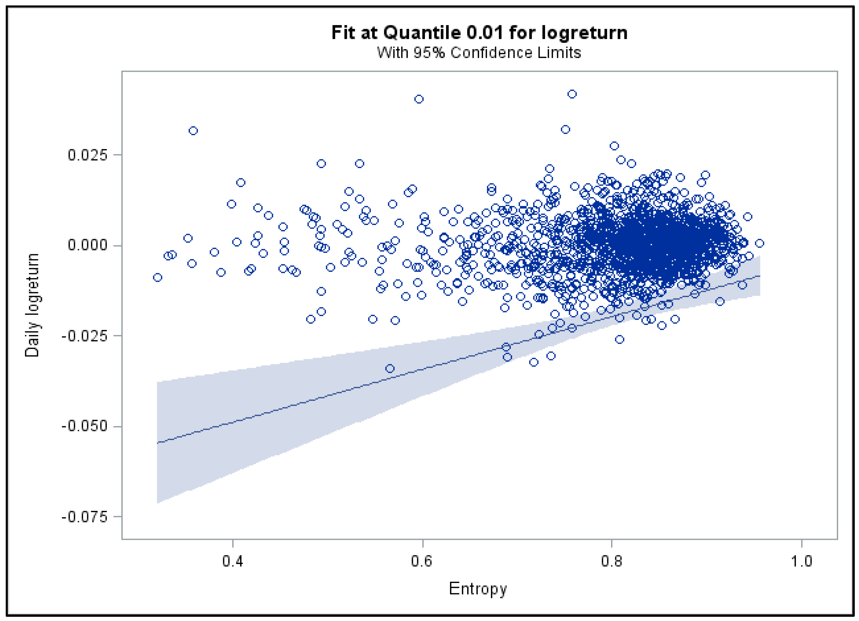
2.2.2. Quantile Regressions for Daily Returns
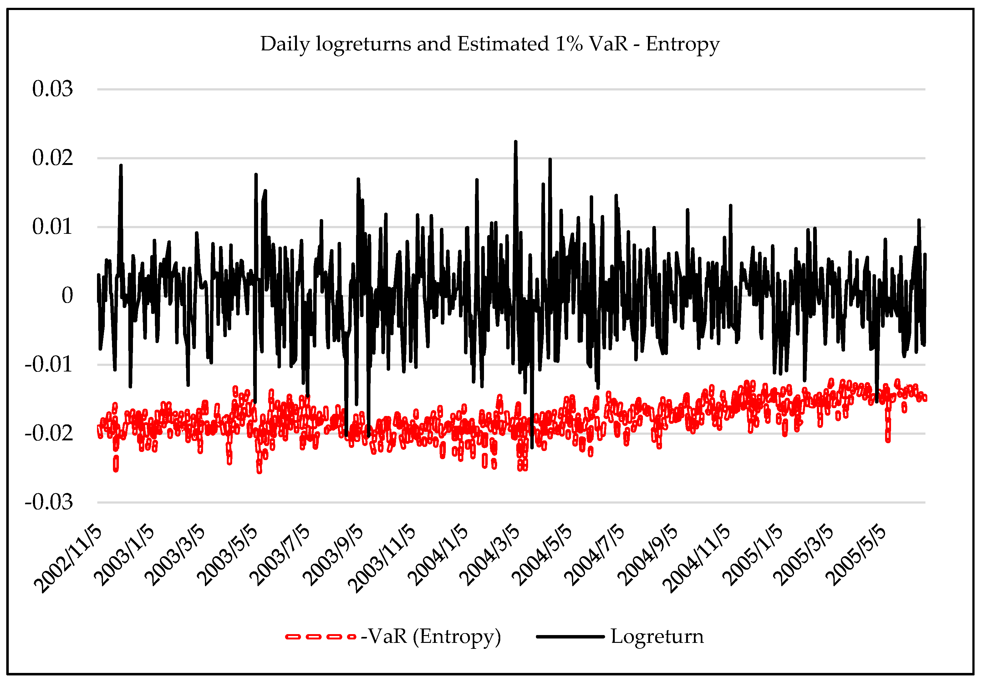
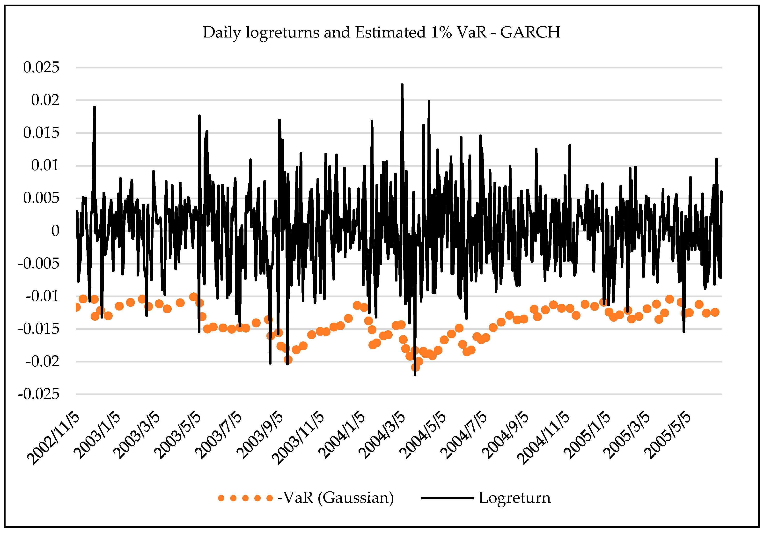
2.3. Forecasting Daily VaR Using Entropy
- Historical VaR forecasts, estimated using a rolling window of length w;
- Normal GARCH(1,1) VaR forecasts, with (17), and forecasting equation (18);
- Student’s t-GARCH(1,1) VaR forecasts, with (17), Student’s t and equation (18);
- Entropy-based VaR forecasts, given by (13) and forecasting equation (14);
- Entropy-based autoregressive VaR forecasts, given in (15) and (16).
3. Empirical Analysis
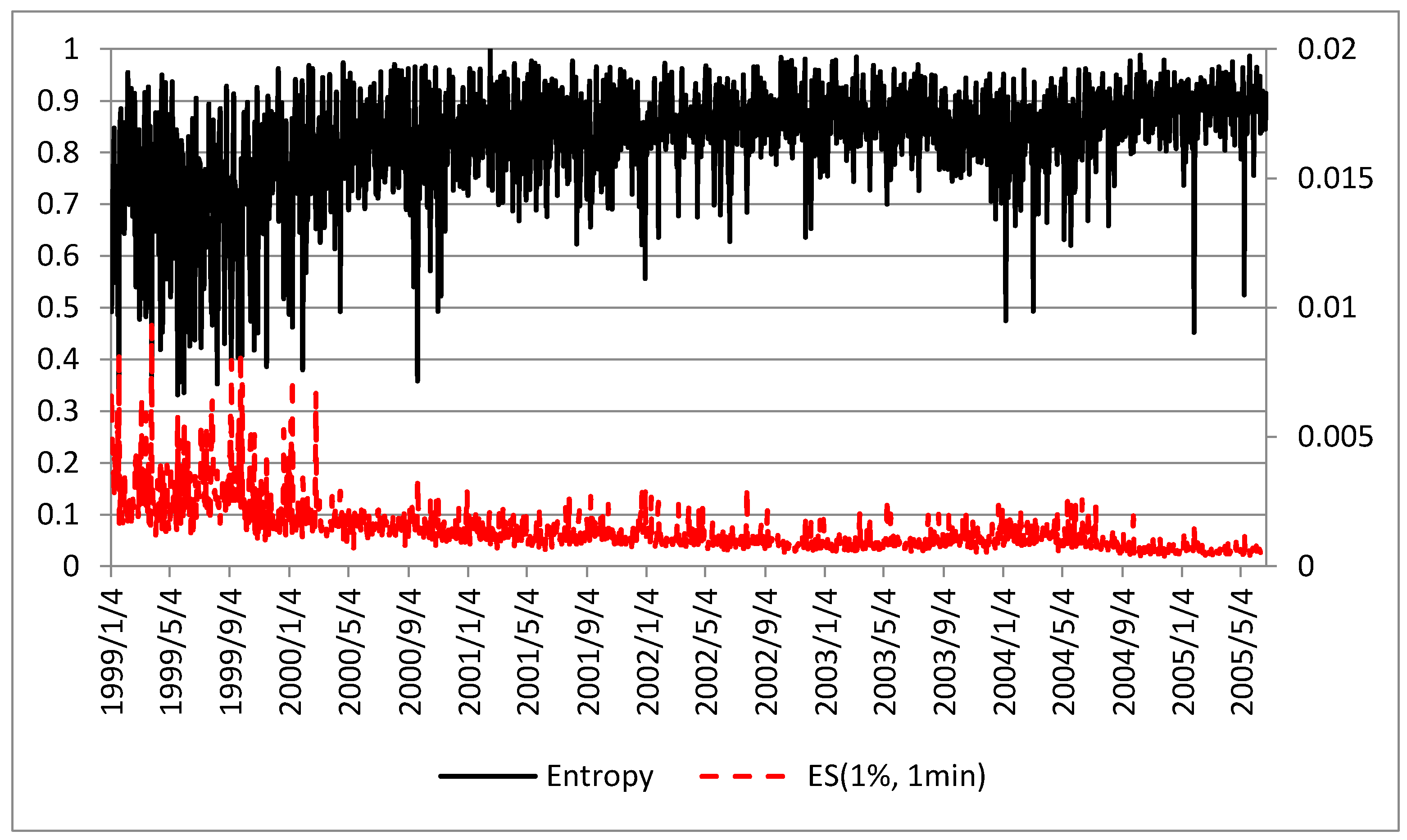
3.1. Entropy and Intraday Measures of Market Risk and Uncertainty
3.2. Quantile Regression Results
3.3. Forecasting Daily VaR Using Entropy
4. Conclusions
Acknowledgments
Author Contributions
Conflicts of Interest
Appendix A. Algorithm for Simulation of Stable Distributions (Weron [34])
Appendix B. VaR Forecasting Tests (Christoffersen [36])
Appendix B.1. The LR Test of Unconditional Coverage
Appendix B.2. The LR Test of Independence
Appendix B.3. The Joint Test of Coverage and Independence
Appendix C. The Diebold-Mariano Test for VaR Forecast Comparisons (Diebold and Mariano [37] and West [38])
References
- Uffink, J. Bluff your way in the second law of thermodynamics. Stud. Hist. Philos. Mod. Phys. 2001, 32, 305–394. [Google Scholar] [CrossRef]
- Avery, J. Information Theory and Evolution, 2nd ed.; World Scientific Publishing: Singapore, 2012. [Google Scholar]
- Zunino, L.; Zanin, M.; Tabak, B.M.; Pérez, D.G.; Rosso, O.A. Forbidden patterns, permutation entropy and stock market inefficiency. Phys. A Stat. Mech. Appl. 2009, 388, 2854–2864. [Google Scholar] [CrossRef]
- Risso, A. The informational efficiency and the financial crashes. Res. Int. Bus. Financ. 2008, 22, 396–408. [Google Scholar] [CrossRef]
- Oh, G.; Kim, S.; Eom, C. Market efficiency in foreign exchange markets. Phys. A Stat. Mech. Appl. 2007, 382, 209–212. [Google Scholar] [CrossRef]
- Wang, Y.; Feng, Q.; Chai, L. Structural evolutions of stock markets controlled by generalized entropy principles of complex systems. Int. J. Mod. Phys. B 2010, 24, 5949–5971. [Google Scholar] [CrossRef]
- Maasoumi, E.; Racine, J. Entropy and predictability of stock market returns. J. Econ. 2002, 107, 291–312. [Google Scholar] [CrossRef]
- Billio, M.; Casarin, R.; Costola, M.; Pasqualini, A. An entropy-based early warning indicator for systemic risk. J. Int. Financ. Mark. Inst. Money 2016, 45, 42–59. [Google Scholar] [CrossRef]
- Dionisio, A.; Menezes, R.; Mendes, D.A. An econophysics approach to analyse uncertainty in financial markets: An application to the Portuguese stock market. Eur. Phys. J. B 2006, 50, 161–164. [Google Scholar] [CrossRef]
- Philippatos, G.C.; Wilson, C. Entropy, market risk and the selection of efficient portfolios. Appl. Econ. 1972, 4, 209–220. [Google Scholar] [CrossRef]
- Ebrahimi, N.; Maasoumi, E.; Soofi, E.S. Ordering univariate distributions by entropy and variance. J. Econ. 1999, 90, 317–336. [Google Scholar] [CrossRef]
- Ebrahimi, N.; Maasoumi, E.; Soofi, E.S. Measuring Informativeness of Data by Entropy and Variance. In Advances in Econometrics: Income Distribution and Methodolgy of Science, Essays in Honor of Camilo Dagum; Springer: Heidelberg, Germany, 1999. [Google Scholar]
- Allen, D.E.; McAleer, M.; Powell, R.; Singh, A.K. A non-parametric and entropy based analysis of the relationship between the VIX and S&P 500. J. Risk Financ. Manag. 2013, 6, 6–30. [Google Scholar]
- Liu, L.Z.; Qian, X.Y.; Lu, H.Y. Cross-sample entropy of foreign exchange time series. Phys. A Stat. Mech. Appl. 2010, 389, 4785–4792. [Google Scholar] [CrossRef]
- Bowden, R.J. Directional entropy and tail uncertainty, with applications to financial hazard. Quant. Financ. 2011, 11, 437–446. [Google Scholar] [CrossRef]
- Gradojevic, N.; Gencay, R. Overnight interest rates and aggregate market expectations. Econ. Lett. 2008, 100, 27–30. [Google Scholar] [CrossRef]
- Gencay, R.; Gradojevic, N. Crash of ’87—Was it expected? Aggregate market fears and long range dependence. J. Empir. Financ. 2010, 17, 270–282. [Google Scholar] [CrossRef]
- Gradojevic, N.; Caric, M. Predicting systemic risk with entropic indicators. J. Forecast. 2017, 36, 16–25. [Google Scholar] [CrossRef]
- Stutzer, M.J. Simple entropic derivation of a generalized Black-Scholes option pricing model. Entropy 2000, 2, 70–77. [Google Scholar] [CrossRef]
- Stutzer, M.J.; Kitamura, Y. Connections between entropic and linear projections in asset pricing estimation. J. Econ. 2002, 107, 159–174. [Google Scholar] [CrossRef]
- Yang, J.; Qiu, W. A measure of risk and a decision-making model based on expected utility and entropy. Eur. J. Oper. Res. 2005, 164, 792–799. [Google Scholar] [CrossRef]
- Ishizaki, R.; Inoue, M. Time-series analysis of foreign exchange rates using time-dependent pattern entropy. Phys. A Stat. Mech. Appl. 2013, 392, 3344–3350. [Google Scholar] [CrossRef]
- Bekiros, S. Timescale analysis with an entropy-based shift-invariant discrete wavelet transform. Comput. Econ. 2014, 44, 231–251. [Google Scholar] [CrossRef]
- Bekiros, S.; Marcellino, M. The multiscale causal dynamics of foreign exchange markets. J. Int. Money Financ. 2013, 33, 282–305. [Google Scholar] [CrossRef]
- Lorentz, R. On the entropy of a function. J. Approx. Theor. 2009, 158, 145–150. [Google Scholar] [CrossRef]
- Zhou, R.; Cai, R.; Tong, G. Applications of entropy in finance: A review. Entropy 2013, 15, 4909–4931. [Google Scholar] [CrossRef]
- Pele, D.T.; Mazurencu-Marinescu, M. Uncertainty in EU stock markets before and during the financial crisis. Econophys. Sociophys. Multidiscip. Sci. J. 2012, 2, 33–37. [Google Scholar]
- Pele, D.T. Information entropy and occurrence of extreme negative returns. J. Appl. Quant. Methods 2011, 6, 23–32. [Google Scholar]
- Silverman, B.W. Density Estimation for Statistics and Data Analysis; Chapman and Hall: London, UK, 1986. [Google Scholar]
- Yamato, H. Uniform convergence of an estimator of a distribution function. Bull. Math. Stat. 1973, 15, 69–78. [Google Scholar]
- Chacón, J.E.; Rodríguez-Casal, A. A note on the universal consistency of the kernel distribution function estimator. Stat. Probab. Lett. 2009, 80, 1414–1419. [Google Scholar] [CrossRef]
- Pele, D.T. Uncertainty and Heavy Tails in EU Stock Markets before and during the Financial Crisis. In Proceedings of the 13th International Conference on Finance and Banking, Lessons Learned from the Financial Crisis, Ostrava, Czech Republic, 12–13 October 2011; pp. 501–512. [Google Scholar]
- Nolan, J.P. Stable Distributions—Models for Heavy Tailed Data; Birkhauser: Boston, MA, USA, 2011. [Google Scholar]
- Weron, R. On the Chambers-Mallows-Stuck method for simulating skewed stable random variables. Stat. Probab. Lett. 1996, 28, 165–171. [Google Scholar] [CrossRef]
- Bandi, F.; Russell, J. Separating microstructure noise from volatility. J. Financ. Econ. 2006, 79, 655–692. [Google Scholar] [CrossRef]
- Christoffersen, P. Evaluating interval forecasts. Int. Econ. Rev. 1998, 39, 841–862. [Google Scholar] [CrossRef]
- Diebold, F.X.; Mariano, R.S. Comparing predictive accuracy. J. Bus. Econ. Stat. 1995, 13, 253–263. [Google Scholar] [CrossRef]
- West, K.D. Asymptotic inference about predictive ability. Econometrica 1996, 64, 1067–1084. [Google Scholar] [CrossRef]
- Giacomini, R.; White, H. Tests of conditional predictive ability. Econometrica 2006, 74, 1545–1578. [Google Scholar] [CrossRef]


| Distribution | Average Value of the Entropy of the Distribution Function | Standard Deviation of the Entropy of the Distribution Function |
|---|---|---|
| Uniform (0,1) | 0.9982 | 0.0011 |
| Normal (0,1) | 0.8933 | 0.0319 |
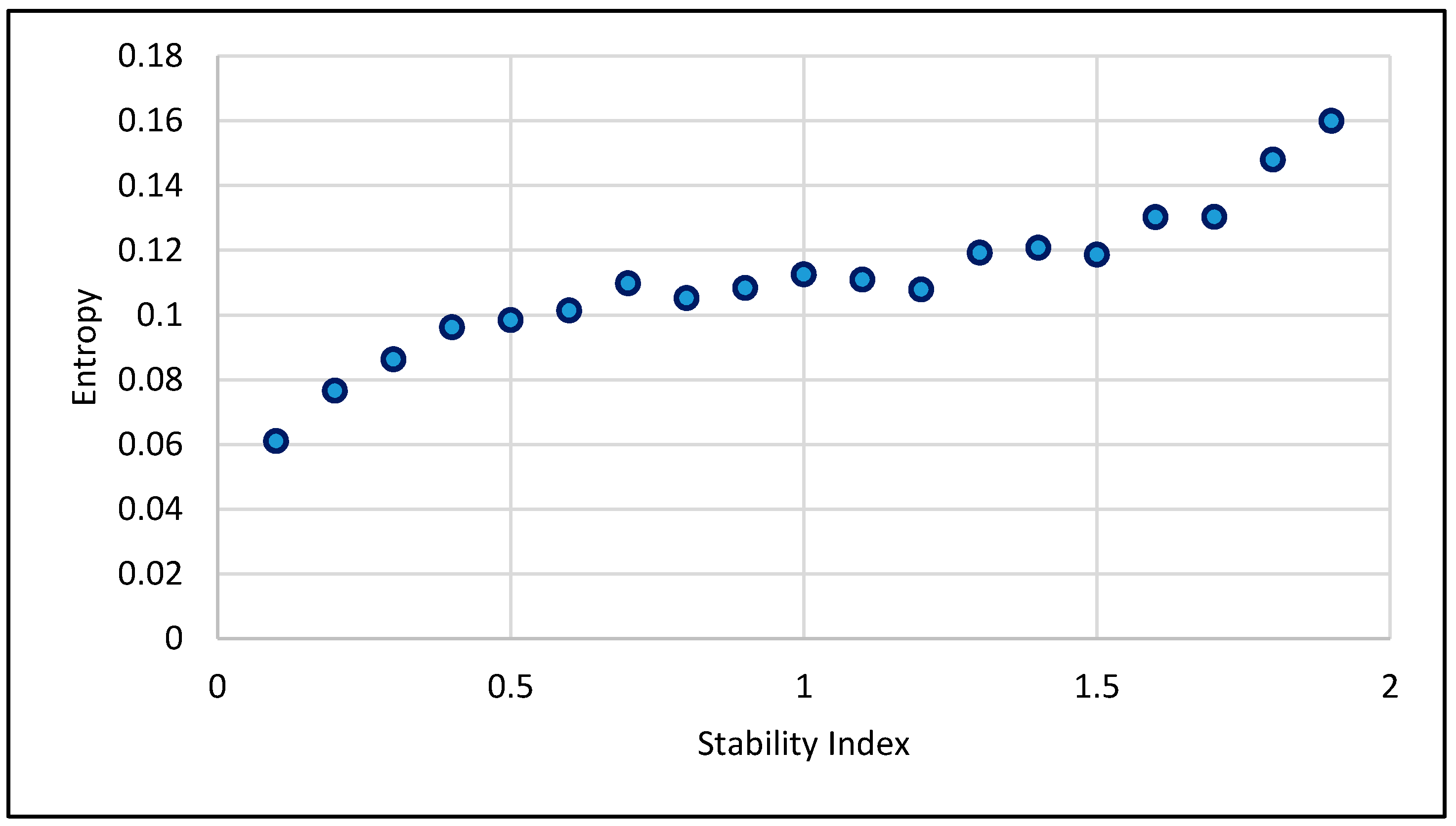
| Stable ( = 1.9) | 0.6725 | 0.1600 |
| Stable ( = 1.5) | 0.4788 | 0.1186 |
| Stable ( = 1) | 0.3979 | 0.1125 |
| Stable ( = 0.5) | 0.2858 | 0.0984 |
| Stable ( = 0.1) | 0.1872 | 0.0610 |
| Sampling Frequency | ν = 1 min | ν = 10 min | ν = 15 min | ||||||
|---|---|---|---|---|---|---|---|---|---|
| Dependent Variable | Dependent Variable | Dependent Variable | |||||||
| Panel A. Static Models | |||||||||
| −0.0050 *** | −0.0070 *** | −0.049 *** | −0.004 *** | −0.7565 *** | −0.044 *** | −0.0089 *** | −1.0669 *** | −0.889 *** | |
| [0.0003] | [0.0003] | [0.0015] | [0.0002] | [0.0205] | [0.0009] | [0.0002] | [0.0234] | [0.0018] | |
| 0.46 | 0.58 | 0.66 | 0.29 | 0.51 | 0.63 | 0.48 | 0.51 | 0.53 | |
| Panel B. Dynamic Models | |||||||||
| 0.5355 *** | - | - | 0.2920 *** | - | - | 0.3687 *** | - | - | |
| [0.0234] | - | - | [0.0351] | - | - | [0.0271] | - | - | |
| - | 0.6024 *** | - | - | 0.1991 *** | - | - | 0.3599 *** | - | |
| - | [0.0262] | - | - | [0.0428] | - | - | [0.0280] | - | |
| - | - | 0.629 *** | - | - | 0.569 *** | - | - | 0.513 *** | |
| - | - | [0.0300] | - | - | [0.0433] | - | - | [0.0280] | |
| −0.0009 *** | −0.0420 *** | −0.001 *** | −0.0011 *** | −0.1607 *** | −0.0003 *** | −0.0017 *** | −0.1835 *** | −0.0002 *** | |
| [0.0002] | [0.0246] | [0.0018] | [0.0003] | [0.0455] | [0.0024] | [0.0004] | [0.0420] | [0.0034] | |
| 0.40 | 0.41 | 0.38 | 0.16 | 0.11 | 0.33 | 0.22 | 0.21 | 0.26 | |
| Panel A. for Intraday VaR | Panel B. for Daily Returns | |||||||
|---|---|---|---|---|---|---|---|---|
| τ = 1% Q for IVaR | τ = 5% Q for IVaR | τ = 1% Q for Returns | τ = 5% Q for Returns | |||||
| Sampling Frequency | ν = 1 min | ν = 10 min | ν = 15 min | ν = 1 min | ν = 10 min | ν = 15 min | Daily | Daily |
| 0.0111 *** | 0.0092 *** | 0.0154 *** | 0.0078 *** | 0.0073 *** | 0.0140 *** | 0.0728 *** | 0.0368 *** | |
| [0.0008] | [0.0012] | [0.0012] | [0.0005] | [0.0005] | [0.0005] | [0.0155] | [0.0075] | |
| Confidence Interval (95%) | 0.0126 | 0.0116 | 0.0177 | 0.0088 | 0.0083 | 0.0150 | 0.1031 | 0.0516 |
| 0.0095 | 0.0068 | 0.013 | 0.0068 | 0.0063 | 0.0131 | 0.0424 | 0.0220 | |
| t-Value | 13.77 | 7.58 | 12.76 | 15.53 | 14.39 | 28.92 | 4.71 | 4.88 |
| Model | Test | p-Value | Test | p-Value | Test | p-Value | |
|---|---|---|---|---|---|---|---|
| Historical VaR | 0.290% | 4.867 ** | 0.027 | 7.443 *** | 0.006 | 12.310 *** | 0.002 |
| n.GARCH(1,1) VaR | 1.597% | 2.097 | 0.148 | 1.658 | 0.198 | 3.755 | 0.153 |
| t-GARCH(1,1) VaR | 0.581% | 1.442 | 0.230 | 5.108 ** | 0.024 | 6.550 ** | 0.038 |
| Entropy VaR | 0.726% | 0.579 | 0.447 | 4.329 ** | 0.037 | 4.908 * | 0.086 |
| Entropy AR VaR | 1.016% | 0.002 | 0.966 | 3.156 * | 0.076 | 3.158 | 0.206 |
| Model | n.GARCH(1,1) VaR | t-GARCH(1,1) VaR | Entropy VaR | Entropy AR VaR |
|---|---|---|---|---|
| Historical VaR | −3.146 *** | −1.004 | −1.755 ** | −2.294 ** |
| n.GARCH(1,1) VaR | - | 2.744 *** | 2.167 ** | 1.428 |
| t-GARCH(1,1) VaR | - | - | −0.448 | −1.141 |
| Entropy VaR | - | - | - | −1.428 |
© 2017 by the authors. Licensee MDPI, Basel, Switzerland. This article is an open access article distributed under the terms and conditions of the Creative Commons Attribution (CC BY) license (http://creativecommons.org/licenses/by/4.0/).
Share and Cite
Pele, D.T.; Lazar, E.; Dufour, A. Information Entropy and Measures of Market Risk. Entropy 2017, 19, 226. https://doi.org/10.3390/e19050226
Pele DT, Lazar E, Dufour A. Information Entropy and Measures of Market Risk. Entropy. 2017; 19(5):226. https://doi.org/10.3390/e19050226
Chicago/Turabian StylePele, Daniel Traian, Emese Lazar, and Alfonso Dufour. 2017. "Information Entropy and Measures of Market Risk" Entropy 19, no. 5: 226. https://doi.org/10.3390/e19050226
APA StylePele, D. T., Lazar, E., & Dufour, A. (2017). Information Entropy and Measures of Market Risk. Entropy, 19(5), 226. https://doi.org/10.3390/e19050226