The Tale of Two Financial Crises: An Entropic Perspective

Abstract

This paper provides a comparative analysis of stock market dynamics of the 1987 and 2008 financial crises and discusses the extent to which risk management measures based on entropy can be successful in predicting aggregate market expectations. We find that the Tsallis entropy is more appropriate for the short and sudden market crash of 1987, while the approximate entropy is the dominant predictor of the prolonged, fundamental crisis of 2008. We conclude by suggesting the use of entropy as a market sentiment indicator in technical analysis.

1. Introduction

In recent years, the applications of entropy in finance and economics have increased considerably. Gell-Mann and Tsallis [1], Tsallis [2] and Tsallis [3] nicely summarize those efforts. Scholarly contributions that link an entropic framework to the field of finance include Ishizaki and Inoue [4], Namaki et al. [5] and Bentes and Menezes [6], while the paper by Gradojevic and Gençay [7] provides an extensive review of major financial applications of the Tsallis entropy. The former papers consider entropy to understand turning points in foreign exchange rate time series [4], to study patterns in the non-extensivity parameter (q) in mature and emerging markets [5] and to propose entropy in stock markets as an alternative to the standard deviation [6]. In other applications, Stutzer [8] and Stutzer and Kitamura [9] study option and asset pricing through an entropic methodology. Entropy-based measures of risk and rare-event probabilities can be found in [10,11]. Applications to forecasting inflation under the maximum entropy principle are described in [12]. An important recent work concerns the application of directional entropy to traditional risk management tools, such as the value-at-risk [13]. Furthermore, two innovative applications of entropy for financial time series forecasting can be found in [14,15]. These papers utilize the Gibbs–Shannon entropy as a measure of decomposing heterogeneous trading horizon-based expectations, in order to forecast aggregate market sentiment (indices) in foreign exchange (FX) markets.

This paper concentrates on discussing and constructing entropic indicators to gauge market sentiment with respect to the 1987 and 2008 financial crises. In our analysis, we argue that the sentiment of a financial market can be summarized through the aggregation of the subjective expectations of its participants. If the expectations of market participants are highly dispersed and independent, extreme price movements are less likely to occur. If however, market participants have highly dependent and less dispersed expectations, the aggregate market sentiment could drive prices to extraordinary levels. Therefore, lack of belief heterogeneity necessitates large market movements and high volatility. Our approach extracts aggregate market expectations from a past sequence of financial option prices via time-dependent entropic methodologies. The entropic indicators we construct thus resemble sentiment indicators based on options and volatility in technical analysis. Such measures include various put-call ratios, option sentiment indices, as well as “fear and greed” and on-balance volume.

The first paper that introduced this idea was [16], followed by [17,18]. The authors of [16] were able to identify strong “abnormal” shifts in the S&P 500 market participants’ aggregate beliefs roughly two months prior to the October 1987 crash. The work in [17] revealed the predictability of the Turkish financial crisis in February 2001, based on the Tsallis entropy of daily overnight interest rates. Quite recently, the authors of [18] demonstrated that the approximate entropy approach could generate predictive signals in advance of the peak of the 2008 subprime mortgage crisis.

In general, the market crisis of 2008 and the crash of 1987 have fundamentally different underlying causes. In the 1987 crash, a sudden news shock occurred three days prior to 19 October and it resulted in a 10% decline in the S&P 500 index [19]. This behaviourally affected the traders to panic and revalue stocks down by more than 20% in one day, while generating an unprecedented trading volume and price volatility. In contrast, the financial crisis of 2008 was driven by a combination of behavioural, macroeconomic, regulatory and supervisory factors. More specifically, the crisis was initiated by the gradual decline in housing prices from their peak in the second quarter of 2006. This trend was combined with the increase in both down payment requirements and purchases of credit default swaps. In September of 2007, this led to the “leverage cycle crisis” in mortgage securities and housing [20]. In other words, the tightening margins in securities produced lower security and housing prices, which further reinforced tighter margins, etc. In the months of August and September 2008 that preceded the peak of the crisis, stock market declined significantly, but the magnitude of the decline and its volatility were still lower than those during the 14–16 October 1987 period. Thus, the crash of 1987 was shorter, more sudden and substantial, whereas the build-up of the crisis of 2008 took place over many turbulent months with its culmination in October 2008. Our goal is to predict the day of the crash in 1987 and the climax of the 2008 crisis that took place from 6–10 October 2008, when the S&P 500 stock market index declined by 18.2%, which represented its worst one-week loss since 1933.

To assess the predictability of aggregate market fears in 1987 and 2008, in this work, we apply time-dependent, entropic measures of the financial market crisis risk from [16,21]. The underlying variables that are used in constructing two different time-varying entropies (Tsallis and approximate entropy) are extracted from a dataset for put and call financial options written on the S&P 500 stock market index. We track aggregate market expectations through the entropic lens ahead and during each of the two crises. The main objective is to study and discuss the applicability of entropies on the 1987 crash that was at its heart more of a market microstructural nature, relative to the fundamental economic crisis of 2008. The results demonstrate that the distribution-free, approximate entropy approach is more appropriate to predict the decline of the S&P 500 stock market index in 2008, while the Tsallis entropy that involves q-Gaussianity is more useful for predicting the 1987 crash.

In Section 2, we provide a brief overview of the Tsallis entropy and the motivation for its use. This is followed by a description of the approximate entropy in Section 3. In Section 4, we present the option data for the S&P 500 index. The results are summarized in Section 5, while the final section concludes the paper.

2. Tsallis Entropy

To motivate the discussion, we consider the probability density function naturally derived from the variational principle related to the Tsallis entropy:

$${\displaystyle S_q\left(p\left(x\right)\right)=k\frac{1-\int {p\left(x\right)}^{q}dx}{q-1}}$$

(1)

where q is a measure of non-additivity, such that $S_q(A\cup B)=S_q\left(A\right)+S_q\left(B\right)-(1-q)S_q\left(A\right)S_q\left(B\right)$, k is a positive constant (k $=1$ or k = $k_B$, where $k_B$ is the Boltzmann constant), and $p\left(x\right)$ is a probability density function.

$S_q$ in its discrete version can be written as:

$${\displaystyle S_q=\frac{1-{\sum }_{i=1}^n{p_i}^q}{q-1}}$$

(2)

where the number of states $i=1,\dots ,n$, $p_i$ is the probability of outcome i and n is the number of states.

One of the advantages of entropy in Equation (1) is that it yields power-law tails, which play an important role in finance. Natural constraints in the maximization of Equation (1) are:

$$\begin{array}{c}\hfill \int p(x)dx=1,\end{array}$$

(3)

corresponding to normalization and:

$$\begin{array}{c}\hfill \int x\frac{{\left[p\left(x\right)\right]}^q}{\int {\left[p\left(x\right)\right]}^{q}dx}dx={\overline{\mu }}_q,\end{array}$$

(4)

$$\begin{array}{c}\hfill \int {(x-{\overline{\mu }}_q)}^q\frac{{\left[p\left(x\right)\right]}^q}{\int {\left[p\left(x\right)\right]}^{q}dx}dx={\overline{\sigma }}_q^2,\end{array}$$

(5)

corresponding to the generalized mean and variance of a relevant quantity x, respectively.

Under the above constraints, one obtains:

$$\begin{array}{c}\hfill p\left(x\right)=A_q{[1+(q-1)B_q{(x-{\overline{\mu }}_q)}^2]}^{\frac{1}{1-q}},q<3,\end{array}$$

(6)

where:

$$\begin{array}{c}\hfill A_q=\frac{\mathsf{\Gamma }\left[\frac{1}{q-1}\right]}{\mathsf{\Gamma }\left[\frac{3-q}{1-q}\right]}\sqrt{\frac{q-1}{\pi }}{B}_q,\end{array}$$

(7)

for the case that is of interest (when $q>1$), and $B_q={\left[(3-q){\overline{\sigma }}_q^2\right]}^{-1}$.

By defining the q-exponential function as:

$$\begin{array}{c}\hfill e_q^x={[1+(1-q)x]}^{\frac{1}{1-q}},\end{array}$$

(8)

one can rewrite Equation (6) as:

$$\begin{array}{c}\hfill p\left(x\right)=A_q{e}_q^{-B_q{(x-{\overline{\mu }}_q)}^2},\end{array}$$

(9)

which is referred to as the q-Gaussian probability density function. The work in [22] proposed this distribution to handle systems with long-range interactions, necessitating a non-extensive generalization of the ordinary Gibbs–Shannon entropy.

The main advantage of this distribution is that in contrast to simple convolutions, which allow only for asymptotic behaviour like q $=1$ (Gaussian) or $q>5/3$ (Lévy distribution) ones, the q-Gaussian distribution allows fat-tailed distributions associated with $1<q\le 5/3$.

As Gaussian distribution is unable to approximate fat tails (or extreme events) that are observed in many high-frequency empirical distributions in finance, we turn our attention to the q-Gaussian probability distribution. Borland [23] shows that the q-Gaussian distribution provides a much better fit to the empirical distribution of the high-frequency S&P 500 index and Nasdaq index returns than the log-normal.

Through a moving window approach, the evolution of $S_q$ for the skewness premium (this variable will be explained in the next section) is calculated over time (see Gamero et al. [24] or Tong et al. [25] for more information). The calculation of a time-dependent entropy is influenced by the following considerations [26]:

• Number of states: With too few states, one may not be able to characterize the underlying market sentiment reliably, and with too many states, tracking fine changes becomes difficult. Without loss of generality, we set n $=10$.
• Partitioning method: There are two different methods for partitioning the range of a time series: (a) fixed partitioning (equipartition is performed on all available data) and (b) adaptive partitioning (equipartition is performed on each moving-window of data, i.e., it changes over time). The adaptive partitioning approach can track transient changes better than the fixed partitioning and is more suitable for our application.
• Estimation of q: The entropic index q is the degree of long-memory in the data. Gell-Mann and Tsallis [1] estimate $q\approx 1.4$ for high-frequency financial data (returns and volumes) and stress that as the data frequency decreases, q approaches unity. Larger q values ($1<q\le 2$) emphasize highly volatile activities in the signal when a time-dependent entropy is plotted against time, i.e., the entropy is more sensitive to possible disturbances in the probability distribution function. In this paper, we find the optimal q by using the maximum likelihood (ML) estimator, as explained in the Results section.
• Sliding step ($\Delta$) and moving window size (K): The sliding step (the number of observations by which the moving window is shifted forward across time) and moving window size (the number of observations used in calculating the entropy) determine the time resolution of $S_q$. If the focus is on tracking the local changes, the sliding step is set to be very small (e.g., one observation: $\Delta$ $=1$). Non-overlapping windows ($\Delta \ge K$) are useful only when one is interested in monitoring the general trend of a time series. To get a reliable probability distribution function, K should not be too small. We set $\Delta$ $=1$, and K is varied from 50–120 days. As demonstrated in [16], the results are unaffected by the (reasonable) choices for the moving-window size (from 50–120 days). The reason we use 50 days in 2008 and 120 days in 1987 is to generate more data points in 2008, given that we could track two years around the other crisis (1987 and 1988).

3. Approximate Entropy

Approximate entropy is an index of complexity or uncertainty, for a given time series [21]. It is based on the likelihood that templates in a time series are similar to the next incremental comparisons. The templates are simply subsequences of the chosen time series. If a time series has a large approximate entropy, i.e., a larger diversity of patterns within a time series, then the time series is associated with a higher uncertainty or higher complexity. Essentially, approximate entropy is a distribution-independent statistic that is insensitive to outliers. It assigns a non-negative number to a time series with greater values corresponding to an increased randomness.

To calculate approximate entropy, the first step is to select a sequence $X=\{x_1,x_2,\dots ,x_N\}$ of length N, which will denote the time series. Then, for $m<N$, let:

$$\begin{array}{c}\hfill u_{\left(m\right)}\left(i\right)=\{x_i,x_{i+1},\dots ,x_{i+(m-1)}\}\end{array}$$

(10)

be an m-dimensional vector, starting at the i-th term in the sequence X.

Let $u_{\left(m\right)}\left(i\right)$ and $u_{\left(m\right)}\left(j\right)$ be two vectors. The distance between the two vectors $u_{\left(m\right)}\left(i\right)$ and $u_{\left(m\right)}\left(j\right)$ of length m is defined as:

$$\begin{array}{c}\hfill d(u_{\left(m\right)}\left(i\right),u_{\left(m\right)}\left(j\right))=max\left\{\right|x_{i+k}-x_{j+k}|:0\le k\le m-1\}.\end{array}$$

(11)

Two vectors $u_{\left(m\right)}\left(i\right)$ and $u_{\left(m\right)}\left(j\right)$ are similar to each other if for some $r>0$,

$$\begin{array}{c}\hfill d(u_{\left(m\right)}\left(i\right),u_{\left(m\right)}\left(j\right))\le r,\end{array}$$

(12)

where r denotes the specified tolerance. Similar vectors are denoted by writing $u_{\left(m\right)}\left(j\right){\sim }^r{u}_{\left(m\right)}\left(i\right)$.

Clearly, the tolerance level r determines the maximum distance between the vectors $u_{\left(m\right)}\left(i\right)$ and $u_{\left(m\right)}\left(j\right)$. Now, in order to determine the number of similar vectors $u_{\left(m\right)}\left(j\right)$ for each of the $N-(m-1)$ vectors $u_{\left(m\right)}\left(i\right)$, the respective distances between the vectors must be measured.

Let $n_{\left(m\right)}\left(i\right)$ denote the number of vectors $u_{\left(m\right)}\left(j\right)$ similar to $u_{\left(m\right)}\left(i\right)$ for a fixed i and m, where:

$$1\le n_{\left(m\right)}\left(i\right)\le N-(m-1).$$

(13)

The relative frequency of finding a vector $u_{\left(m\right)}\left(j\right)$ in the sequence X that is similar to $u_{\left(m\right)}\left(i\right)$ within a tolerance level r is defined as:

$$C_{\left(m\right)}\left(u_{\left(m\right)}\left(i\right)\right|X,r)=\frac{n_{\left(m\right)}\left(i\right)}{N-(m-1)}.$$

(14)

Note that by Equation (13), it is clear that:

$$\begin{array}{c}\hfill \frac{1}{N-(m-1)}\le C_{\left(m\right)}\left(u_{\left(m\right)}\left(i\right)\right|X,r)\le 1.\end{array}$$

(15)

Then, the average frequency of the logarithm of $C_{\left(m\right)}\left(u_{\left(m\right)}\left(i\right)\right|X,r)$ must be considered in the approximate entropy calculations.

The average frequency of the logarithm of Equation (14) is defined as:

$${\mathsf{\Phi }}_{\left(m\right)}\left(r\right)=\frac{1}{N-(m-1)}\sum _{i=1}^{N-(m-1)}ln\left(C_{\left(m\right)}\left(u_{\left(m\right)}\left(i\right)\right|X,r)\right).$$

(16)

Now, using Equation (16), the approximate entropy algorithm may be defined.

The approximate entropy of length m and sequence X with a tolerance level r is defined as:

$$ApE{n}_{\left(m\right)}\left(r\right):=\underset{N\to \infty }{lim}({\mathsf{\Phi }}_{\left(m\right)}\left(r\right)-{\mathsf{\Phi }}_{(m+1)}\left(r\right)).$$

(17)

Next, the approximate entropy for a sequence X with a finite length N can be determined using Equation (17).

Let r denote the specified tolerance and m denote the dimension of the vectors $u_{\left(m\right)}\left(i\right)$. For a finite sequence of length N, the approximate entropy is estimated by statistics using the following function:

$$\begin{array}{c}\hfill ApE{n}_{\left(m\right)}(r,N):={\mathsf{\Phi }}_{\left(m\right)}\left(r\right)-{\mathsf{\Phi }}_{(m+1)}\left(r\right).\end{array}$$

(18)

The parameters that are required to calculate the approximate entropy must be specified. Recall that N is the length of the randomly-chosen time series or sequence; m denotes the dimension of the vectors $u_{\left(m\right)}\left(i\right)$; and r is the specified tolerance level. In our analysis, N denotes the length of the moving window, which will be similar to K for the Tsallis entropy, for the comparison purposes. Following [21], we set m $=2$ and $r=0.15\times \sigma$, where $\sigma$ represents the standard deviation of the time series.

4. Data

The data are provided by DeltaNeutral and represent the daily S&P 500 index European option prices, taken from the Chicago Board Options Exchange. Call and put options across different strike prices and maturities are considered for 1987 and 2008. In 2008, there are 173,426 put options and 173,403 call options in the sample, i.e., on average, about 690 put or call options are traded daily. The data for 1987 were taken from [16], and the sample is smaller with roughly 8000 pairs of put and call options for which we extract the deepest out-of-the-money options. Since it is one of the deepest and the most liquid option markets in the United States, the S&P 500 index option market is sufficiently close to the theoretical setting of the Black–Scholes model.

We calculate the underlying variable (daily skewness premium), and then, by using a moving-window technique, we sequentially estimate the corresponding time-dependent Tsallis entropy for each moving window. The definition of skewness premium (x) follows Gençay and Gradojevic [16], and we use it for all available European options:

$$x=\frac{P(S,T,K_p)}{C(S,T,K_c)}-1,$$

(19)

where P is the put option premium, C is the call option premium, S is the price of the underlying (S&P 500 index), T is maturity and $K_c$ and $K_p$ are strike prices for the deepest available out-of-the-money call and put options, respectively. Hence, we match put and call options of the same maturity and strike price and use their prices to calculate the skewness premium.

5. Results

5.1. 2008 Crisis

First, we estimate the long memory parameter ($\widehat{q}$) based the first two quarters of 2008 (sample period before the crisis) by using the ML estimator as follows:

$$q=\underset{q}{argmax}\prod _{i=1}^{T}p\left(x_i\right|q)=\underset{q}{argmax}\sum _{i=1}^{T}logp\left(x_i\right|q),$$

(20)

where T is the sample size.

We find that $\widehat{q}$ = 1.62 (0.04) (the number in parentheses is the bootstrap standard error; we use one leave-out bootstrap with replacement for a window size of K $=50$ observations). Using the optimal q, next, we investigate the evolution of the time-dependent Tsallis entropy based on the underlying variable, skewness premium (x).

Table 1. Distribution of the aggregate market expectations for skewness premium in 2008.

Date	${\mathit{s}}_1$	${\mathit{s}}_2$	${\mathit{s}}_3$	${\mathit{s}}_4$	${\mathit{s}}_5$	${\mathit{s}}_6$	${\mathit{s}}_7$	${\mathit{s}}_8$	${\mathit{s}}_9$	${\mathit{s}}_{10}$	TE
1 April 2008	0.3	0.2	0.1	0.2	0.06	0.02	0.04	0.04	0.02	0.02	1.397
1 May 2008	0.24	0.22	0.28	0.2	0.02	0.02	0	0	0	0.02	1.236
2 June 2008	0.18	0.42	0.26	0.08	0.02	0.02	0	0	0	0.02	1.130
1 July 2008	0.56	0.22	0.08	0.06	0.02	0.02	0	0	0.02	0.02	1.005
1 August 2008	0.08	0.72	0.02	0.04	0.06	0.04	0	0	0.02	0.02	0.784
15 August 2008	0.02	0.74	0	0	0	0.02	0	0	0.02	0.02	0.606
2 September 2008	0.22	0.62	0.08	0	0	0	0.02	0.02	0.02	0.02	0.869
15 September 2008	0.24	0.46	0.24	0	0	0	0	0.02	0.02	0.02	1.014
1 October 2008	0.30	0.50	0.10	0.02	0	0.02	0	0.02	0.02	0.02	1.012
8 October 2008	0.48	0.32	0.08	0.04	0	0.02	0	0.02	0.02	0.02	1.033
9 October 2008	0.76	0.10	0.04	0.02	0.02	0.02	0.02	0	0	0.02	0.679
10 October 2008	0.90	0.06	0.02	0	0	0	0	0	0	0.02	0.299
15 October 2008	0.86	0.04	0.02	0	0.02	0	0	0	0.02	0.04	0.430
3 November 2008	0.80	0.04	0.04	0.04	0.02	0	0	0	0.02	0.04	0.595
1 December 2008	0.80	0.04	0.04	0.04	0.02	0	0	0	0.02	0.04	0.595

Notes: The time-dependent Tsallis entropy (TE) is calculated with a moving window of 50 days for the skewness premium (x). $s_1,\dots ,s_{10}$ denote non-overlapping intervals (states). The lower boundary of $s_1$ is the minimum of the moving window. Accordingly, the upper boundary of $s_{10}$ is the maximum of the moving window. Aggregate expectation probabilities ($p_i$) are calculated from the ratio between the number of observations in each interval and the total number of observations in the moving window. The maximum entropy (expectations heterogeneity) corresponds to equal probability of 10% for each state. The minimum entropy (expectations homogeneity) occurs when all observations concentrate in one particular state such that one state receives 100% of the probability. In this particular case above, one can observe how the distribution of expectations converges to states $s_1,\dots ,s_3$ in the months prior to the peak of the crisis (10 October 2008, according to the entropic framework). The increased concentration leads to a reduction in the entropy.

presents how the probabilities of the states are distributed before and during the crisis based on the skewness premium (x). Before April, 2008, the probabilities were relatively evenly distributed across the states, although more weight can be found in states $s_1$–$s_5$. In the subsequent period, a convergence towards states $s_1$–$s_3$ can be observed, and large probability values are located in states $s_1$ and $s_2$. For example, on 1 July 2008, the first two states carry a combined probability of 0.78. The redistribution of probabilities is followed by a declining trend in the entropy values. This trend is strong until 15 August 2008, when the entropy dips to 0.606 and the market concerns are at their highest level since the beginning of 2008. The probabilities remained concentrated in states $s_1$ and $s_2$ until 10 October 2008, when, according to our framework, the financial crisis reaches its peak and the first state received 90% of the probabilities. The movements in the entropy along with the skewness premium can be tracked in Figure 1. As the financial crisis was evident in September of 2008 and the major stock market indices recorded the largest losses in October of 2008, we consider the strong concentration of probabilities on 15 August 2008, as well as their subsequent stable distribution to be a confirmation of the predictive ability of our methodology.

Although the results presented above reveal major shifts in aggregate market expectations and systemic risk ahead of October 2008, the fact that the Tsallis entropy recovers from its local minimum of 15 August 2008 can be interpreted as a noisy signal regarding the predictability of the crisis (Figure 1). In [16], the early warning signal produced by the Tsallis entropy involved a strong decline about two months prior to the market crash, followed by low and stable entropy values until the crash date. Clearly, our framework shows that the Tsallis entropy is more accurate in predicting the one-day crash in 1987 than the peak of the crisis in 2008.

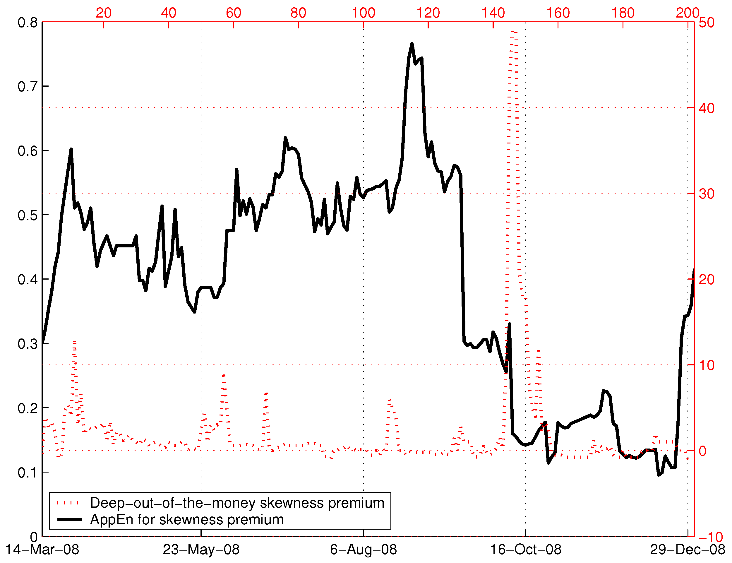
To investigate whether it is possible to obtain greater predictability, next, we employ the approximate entropy in the spirit of [21] while the skewness premium remains the underlying variable. Figure 2 depicts the fluctuations in the skewness premia and the resulting approximate entropy. The feature that stands out is that they resemble [16] with respect to the plunge of entropy in the period before the crisis (the results are not materially different when we vary the moving window size between $K=25$ and $K=75$).

5.2. 1987 Crash

In this subsection, we analyse the daily S&P 500 index European put and call option prices from the Chicago Board Options Exchange. The dataset (this is the dataset used in [27]) contains options across different strike prices and maturities over the period from January 1987–December 1988. The estimate of the long-memory parameter ($\widehat{q}$) for the deepest out-of-the-money options is 1.53 (0.04) (the number in parentheses is the bootstrap standard error; we use one leave-out bootstrap with replacement for a window size of K = 120 observations).

We first investigate the evolution of Tsallis entropy based on the skewness premium for the deepest out-of-the-money options. These findings are the most striking where an early indication of the lack of belief dispersion surfaced on 25 August 1987 (Figure 3), two months prior to the crash. Moreover, after this substantial decrease from 0.92 down to 0.02, the entropy remained at a relatively stable level of 0.27 until the time of the crash and only going down to 0.26 on the day of the crash. The distribution of the probabilities for the states also converged to state $s_1$ on 25 August 1987 (

Table 2. Distribution of aggregate market expectations for skewness premium in 1987.

Date	${\mathit{s}}_1$	${\mathit{s}}_2$	${\mathit{s}}_3$	${\mathit{s}}_4$	${\mathit{s}}_5$	${\mathit{s}}_6$	${\mathit{s}}_7$	${\mathit{s}}_8$	${\mathit{s}}_9$	${\mathit{s}}_{10}$	TE
20 August 1987	0.53	0.19	0.06	0.04	0.04	0.03	0.00	0.07	0.01	0.03	0.92
21 August 1987	0.53	0.19	0.05	0.04	0.04	0.03	0.00	0.07	0.02	0.03	0.91
24 August 1987	0.53	0.20	0.04	0.04	0.04	0.03	0.00	0.07	0.02	0.03	0.92
25 August 1987	0.99	0.00	0.00	0.00	0.00	0.00	0.00	0.00	0.00	0.00	0.02
26 August 1987	0.99	0.00	0.00	0.00	0.00	0.00	0.00	0.00	0.00	0.01	0.04
27 August 1987	0.99	0.00	0.00	0.00	0.00	0.00	0.00	0.00	0.00	0.01	0.06
16 September–16 October 1987	0.89	0.05	0.01	0.02	0.02	0.00	0.00	0.00	0.00	0.01	0.27
19 October 1987	0.89	0.05	0.01	0.03	0.01	0.00	0.00	0.00	0.00	0.01	0.26

Notes: The time-dependent Tsallis entropy (TE) is calculated with a moving window of 120 days for the S&P 500 average skewness premium. $s_1,\dots ,s_{10}$ denote non-overlapping intervals (states). The lower boundary of $s_1$ is the minimum of the moving window. Accordingly, the upper boundary of $s_{10}$ is the maximum of the moving window. Belief probabilities ($p_i$) are calculated from the ratio between the number of observations in each interval and the total number of observations in the moving window. The maximum entropy (belief heterogeneity) corresponds to equal probability of 10% for each state. The minimum entropy (belief homogeneity) occurs when all observations concentrate in one particular state such that one state receives 100% of the probability. In this particular case above, belief distribution is spread out in states $s_1$–$s_{10}$ on 20 August 1987. The concentration increases towards $s_1$ on 25 August, leading the entropy to fall to 0.02 from 0.92. The concentration in $s_1$ remains until the day of the crash. The entropy is bounded between [0, 1.23] for $q=1.62$.

). In this particular case, the deepest out-of-the-money options are informative regarding the extreme expectations, and the entropy provides a useful platform to measure the concentration of these expectations in a particular direction.

Figure 4 displays the approximate entropy of the skewness premium for 1987. A similar pattern emerges on 25 August 1987, but, in contrast to Figure 3, the entropy first plunges to roughly 0.4, and then, it slowly drops to 0.2, where it remains stable until the crash. We conclude that Tsallis entropy generates a more striking warning signal of sudden, “abnormal” shifts in the S&P 500 market participants’ beliefs prior to the crash. This is because the q-Gaussian probability distribution is by definition more sensitive to extreme shifts in market sentiment. Remarkably, both entropies remain low at the value of about 0.2 in the 3–4 weeks immediately preceding the crash.

5.3. Entropy and Technical Analysis

In this work, we define the entropic indicators based on put and call option prices as reflective of aggregate market expectations, i.e., market sentiment. In technical analysis, market sentiment refers to the psychology or the emotion of market participants [28]. Investors react emotionally to the market movements, while their reactions can affect the market. Hence, the causality may exist in both directions. We will consider two popular sentiment indicators, “fear and greed” (FG) and on-balance-volume (OBV), and they will be compared to both Tsallis and approximate entropies in 2008.

FG is a proprietary indicator from Bloomberg that measures the momentum behind price movements, based on the daily ‘true’ trading range. The “true” range represents today’s trading range, adjusted for the gap between yesterday’s close and today’s open (i.e., the greatest of (a) today’s high minus today’s low; (b) the absolute value of today’s high minus yesterday’s close; (c) the absolute value of today’s low minus yesterday’s close). The average true range (ATR) is an exponential average of these values over time. The FG indicator is the spread of two differently-weighted ATRs. It is calculated in a way that it oscillates on a zero base line. Positive (negative) values of the indicator identify when price volatility is supporting a bullish (bearish) trend. The OBV measure compares the closing price and cumulates daily volume according to the sign of daily returns. If the current (i.e., from ($t-1$) to t) S&P 500 index return is positive (negative), to calculate OBV${}_t$, the current volume is added to (subtracted from) OBV${}_{t-1}$. If the closing price equals the prior close price then OBV${}_t$ = OBV${}_{t-1}$. OBV monitors market sentiment, and in theory, its changes should precede price changes. We will also calculate daily changes in FG and OBV, denoted by $\Delta$FG and $\Delta$OBV, respectively.

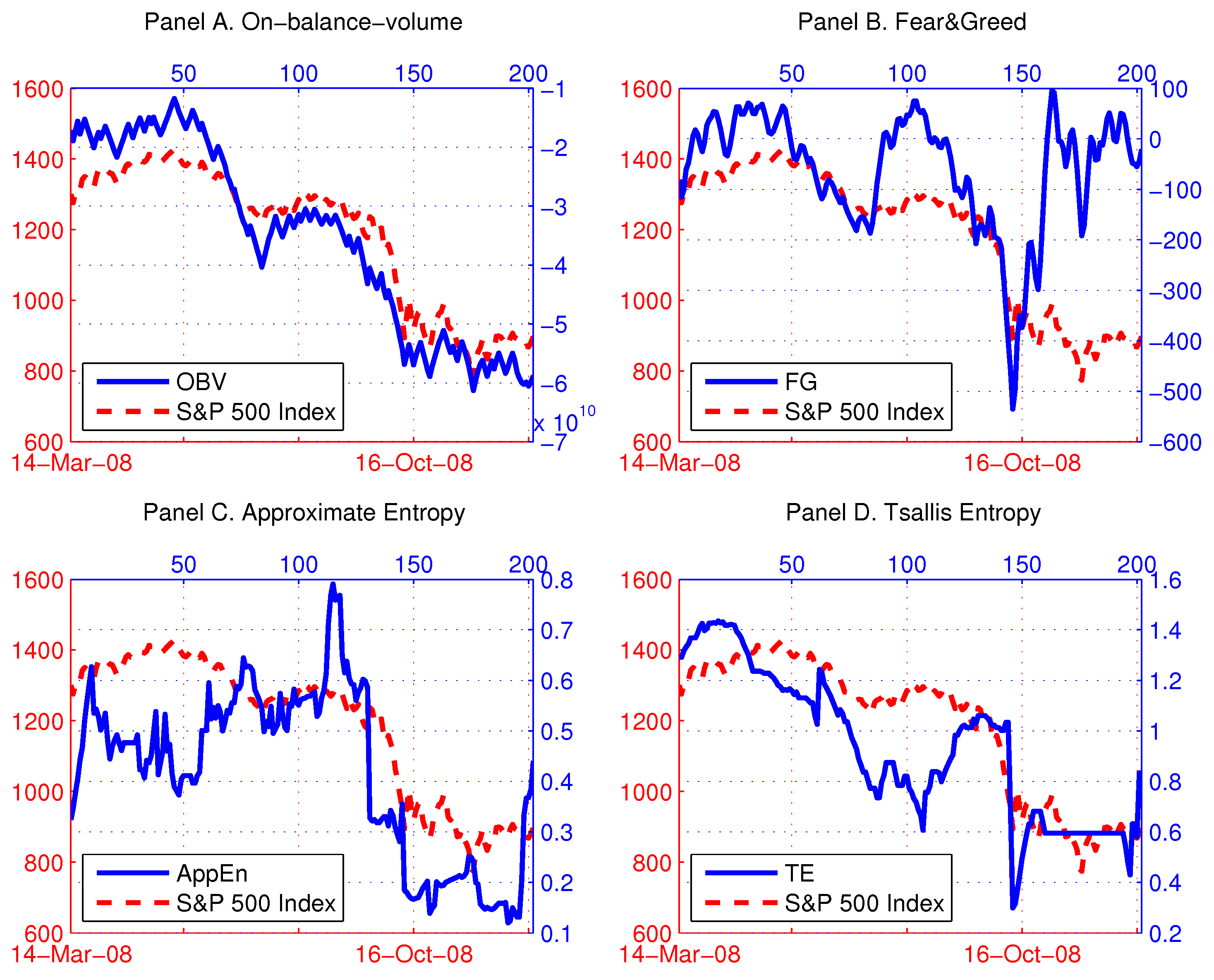
Figure 5 shows the time series plots of the S&P 500 index, OBV, FGand the two entropies in 2008. From Panels A and B, we can conclude that technical indicators are quite successful in tracking the contemporaneous changes of the S&P 500 index. This cannot be observed for the entropies, and they appear not to be moving in tandem with the market movements (Panels C and D). Nevertheless, rather than studying correlations, we are more interested in the potential predictive content of the technical indicators and the entropies for the S&P 500 index. Thus, we run Granger causality tests, and we present the results in

Table 3. Granger causality tests.

Null Hypothesis	${\mathit{\chi }}^{\mathbf{2}}$	Prob $\mathbf{>}{\mathit{\chi }}^{\mathbf{2}}$	$\mathit{n}\mathbf{\left(}\mathit{lag}\mathbf{\right)}$
$\Delta$OBV does not cause S&P 500 index daily returns	3.08	0.378	198
S&P 500 index daily returns does not cause $\Delta$OBV	14.27	0.003	(3)
$\Delta$FG does not cause S&P 500 index daily returns	8.12	0.044	198
S&P 500 index daily returns does not cause $\Delta$ FG	16.96	0.001	(3)
$\Delta$TE does not cause S&P 500 index daily returns	35.44	0.000	193
S&P 500 index daily returns does not cause $\Delta$ TE	15.68	0.047	(8)
$\Delta AppEn$ does not cause S&P 500 index daily returns	17.61	0.001	198
S&P 500 index daily returns does not cause $\Delta AppEn$	3.97	0.264	(3)

Notes: This table lists the probabilities from Granger causality tests in relation to the S&P 500 index daily returns. The time series are on-balance-volume daily change ($\Delta$OBV), “fear and greed” daily change ($\Delta$FG), approximate entropy daily change ($\Delta AppEn$) and Tsallis entropy daily change ($\Delta$TE). The test statistic is distributed as ${\chi }^2(df=2)$, with critical value ${\chi }_{cr}^2$ = 5.991 for the 5% significance level. The null hypothesis is stated in the first column. The estimations are based on a standard bivariate framework. The figures in the third column are the probabilities of rejection. The number of observations (The Akaike information criterion (AIC) optimal lag length) is denoted by $n\left(lag\right)$ and is shown in the last column.

. Essentially, the Granger causality test assesses the ability of one series to forecast another, and this is the primary motivation for using technical indicators as predictors of stock market returns.

In the first two rows of Table 3, we test the predictive ability of the classical technical indicators, OBV and FG. The causal relationship between OBV and the S&P 500 index exhibits statistically significant (at the 1% significance level) reverse causality from the S&P 500 index returns to the changes in OBV, and not vice versa. Contrary to the theoretical expectation, OBV is unsuccessful in forecasting stock market returns. Moreover, it is lagging the market fluctuations. Meanwhile, at the 5% significance level, we reject the null hypothesis that FG does not cause S&P 500 index daily returns. In addition, the reverse causality from the S&P 500 index to FG is statistically significant at the 1% significance level. These results support the weak version of the efficient market hypothesis and seriously undermine the usefulness of FG and OBV in technical trading.

More encouraging results emerge from the third and fourth row of Table 3, where we consider the usefulness of entropy as a sentiment indicator. Both entropies are found to Granger cause the S&P 500 index daily returns at the 1% significance level. In the case of TE, there seems to exist a slight impact of the S&P 500 index returns on the TE changes, but it is not statistically significant at the 1% significance level. Further, $AppEn$ demonstrates its dominant ability to predict S&P 500 index returns, with no evidence of reverse causality. This is in agreement with our findings from the previous two subsections. Overall, sentiment indicators based on entropy are superior to OBV and FG in providing the early warning signals of abnormal shifts in investor sentiment in 2008.

To corroborate the Granger causality tests, we also run predictive regressions and calculate the out-of-sample test statistics to compare the predictability of different market sentiment indicators including the entropic measures. We run the following regression for each predictor $x_t$ ($x_t\in \{\Delta$OBV, $\Delta$FG, $\Delta AppEn$, $\Delta$TE}):

$$\Delta S{P}_t=\alpha +\beta x_{t-lag}+{ϵ}_t,$$

(21)

where $\Delta S{P}_t$ is the daily return on the S&P 500 index and “lag” denotes the optimal lag length for predictors as indicated in Table 3.

The out-of-sample tests are conducted on the last 100 available observations in 2008, whereas the first in-sample observation starts on the 50th day of the year, given that we generate the first entropy value from a 50-day moving-window. Hence, our in-sample and out-of-sample periods are roughly the same size. We estimate the out-of-sample predictions by using the recursive estimation scheme where the size of the initial estimation sample grows for each successive prediction, until we exhaust the out-of-sample data.

Table 4. Predictive regressions.

Regressor (${\mathit{x}}_{\mathit{t}}$)	$\mathbf{\Delta }$OBV	$\mathbf{\Delta }$FG	$\mathbf{\Delta }$$\mathit{AppEn}$	$\mathbf{\Delta }$TE
$MSPE$	6.6781	6.8730	6.0965	6.6398
$PERC$	54%	49%	60%	54%

Notes: This table lists the $MSPE$ and $PERC$ out-of-sample statistics calculated from the predictive regression (Equation (21)). The regressors are lagged on-balance-volume daily change ($\Delta$OBV), “fear and greed” daily change ($\Delta$FG), approximate entropy daily change ($\Delta$$AppEn$) and Tsallis entropy daily change ($\Delta$TE). The regressand is the daily return on the S&P 500 index ($\Delta$SP${}_t$). All $MSPE$ figures have been multiplied by 10${}^4$.

summarizes the results for all four model specifications and displays the mean squared prediction errors ($MSPE$) and the $PERC$ statistic that counts the total number of correctly-forecasted positive and negative movements, defined as: $PERC$ = (number of positive correct responses + number of negative correct responses)/(out-of-sample size). Clearly, the predictive regression that uses $\Delta AppEn$ as a regressor is the most dominant in terms of both out-of-sample test statistics.

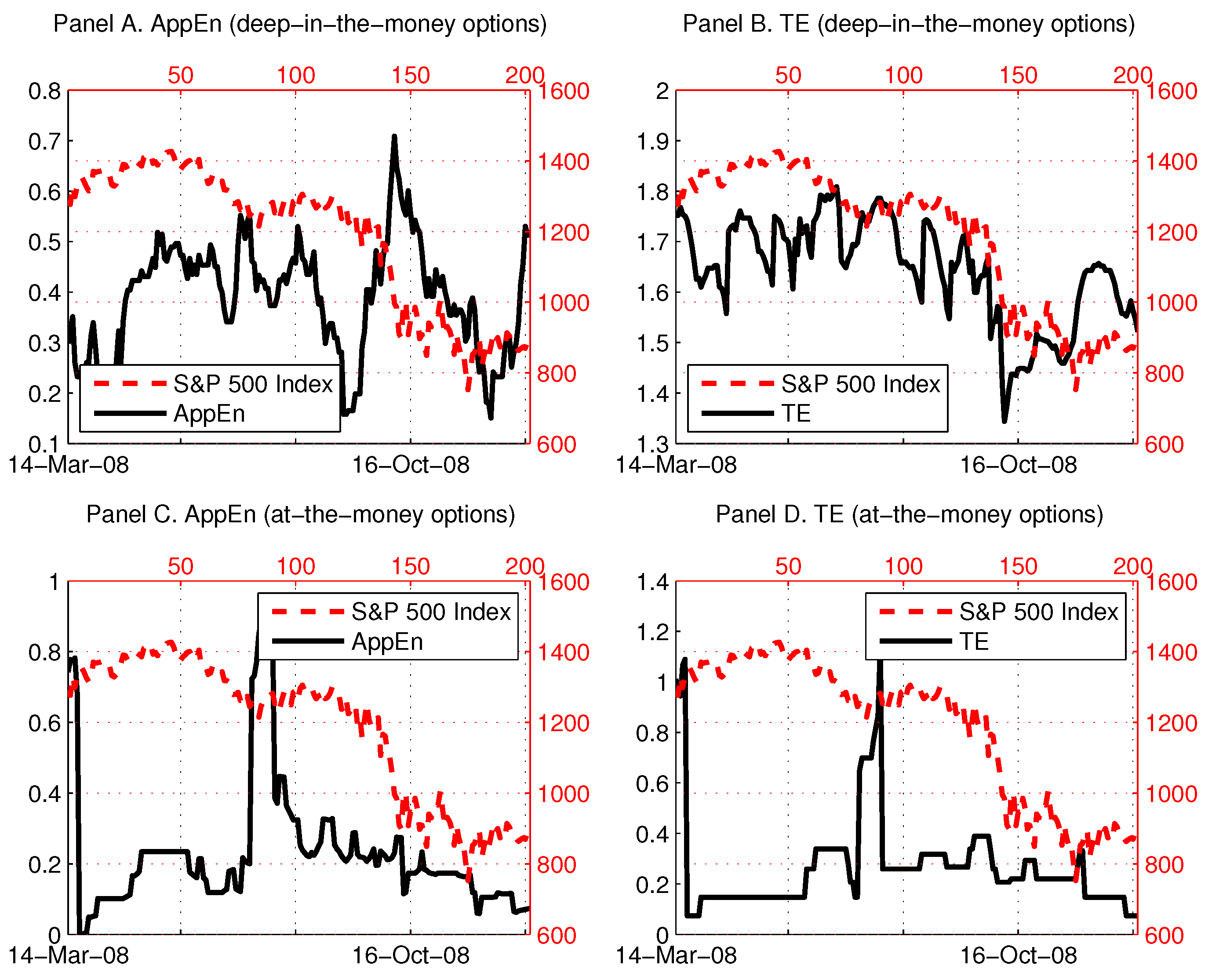
In our analysis, we use the deepest available out-of-the-money call and put options. In [16], we also calculated an entropic measure based on the average skewness premium of all available options (at-, in- and out-of-the-money options), and that deteriorated the results. We conclude that the informational content of in-the-money and at-the-money options is noisier and inferior to that of out-of-the-money options. This could be explained as, when an option is in-the-money or at-the-money (i.e., immediately exercisable or close to that), the price mark-up of such an option over an out-of-the-money option depends primarily on the cash flows of the underlying asset and only secondarily on the skewness of its distribution (that determines aggregate market expectations). To support this argument, we plot the two entropies for the skewness premia of the deepest in-the-money and at-the-money options and compare them to the S&P 500 index in 2008 (Figure 6). We do not observe any predictable patterns or early warning signals in the four panels of Figure 6, especially from the at-the-money options (Panels C and D). In Panel A, the approximate entropy appears to be lagging the movements of S&P 500 index, while, in Panel B, the Tsallis entropy tracks the S&P 500 index contemporaneously.

6. Conclusions

This paper utilizes a time-dependent entropy approach in order to obtain an early indication of the 1987 and 2008 financial crises. We extract the entropy from the daily skewness premia for the put and call European options that were traded in 1987 and 2008. The results show that the entropic methodology performs well in tracking aggregate market expectations and generating early warning signals of excessive shifts in market sentiment; it represents a dominant and viable alternative to classical sentiment indicators in technical analysis. Consequently, we envision the usage of entropic sentiment indicators for the analysis of real-time financial market data as part of services such as Bloomberg Terminals and Thomson Reuters Eikon platforms. In light of our findings, we consider entropic indicators to be more general and informative than the existing sentiment indicators (e.g., Erlanger put/call ratio) that are available at these platforms.

A valuable insight of this paper is that we directly compare the Tsallis entropy and the approximate entropy. We find that the Tsallis entropy is more appropriate in cases when the market movements are sudden and extreme such as in the crash of 1987. Large variability requires a non-extensive generalization of the ordinary Gibbs–Shannon entropy and q-Gaussianity. On the other hand, the crisis of 2008 reveals that a distribution-free entropic approach for quantifying market sentiment is more useful.

The economic intuition of the appropriateness of a certain entropy type could be compared to the usage of non-parametric vs. parametric models. Typically, non-parametric models offer superior out-of-sample performance relative to parametric models due to the restrictive functional shapes used by parametric benchmarks. In contrast, non-parametric models provide flexibility by allowing a variety of cumulative distributions that effectively accommodate jumps, non-stationarity and negative skewness and kurtosis. In the fundamental economic crisis of 2008, the predictive flexibility was obtained from the distribution-free approximate entropy. On the contrary, the Tsallis entropy is restricted by the fat-tailed q-Gaussian probability distribution that performs well when the market makes extreme moves such as in the 1987 crash.

Although our results have direct applications to financial risk management, within the context of technical trading and sentiment indicators, our future research will seek to test the reliability and economic value of entropy-based trading strategies. These explorations will cover various underlying asset classes (and markets) over multiple time periods of both financial distress and stability. A range of alternative sentiment indicators in charting will be compared to our trading strategies. Finally, we will attempt to methodologically improve our approach by relying on other types of entropy that include sample entropy, Rényi entropy and spectral entropy.

References

- Gell-Mann, M.; Tsallis, C. Nonextensive Entropy: Interdisciplinary Applications; Oxford University Press: Oxford, UK, 2004. [Google Scholar]
- Tsallis, C. Introduction to Nonextensive Statistical Mechanics: Approaching a Complex World; Springer: New York, NY, USA, 2009. [Google Scholar]
- Tsallis, C. The nonadditive entropy Sq and its applications in physics and elsewhere: Some remarks. Entropy 2011, 13, 1765–1804. [Google Scholar] [CrossRef]
- Ishizaki, R.; Inoue, M. Time-series analysis of foreign exchange rates using time-dependent pattern entropy. Phys. A Stat. Mech. Appl. 2013, 392, 3344–3350. [Google Scholar] [CrossRef]
- Namaki, A.; Lai, Z.K.; Jafari, G.; Raei, R.; Tehrani, R. Comparing emerging and mature markets during times of crises: A non-extensive statistical approach. Phys. A Stat. Mech. Appl. 2013, 392, 3039–3044. [Google Scholar] [CrossRef]
- Bentes, S.; Menezes, R. Entropy: A new measure of stock market volatility? J. Phys. Conf. Ser. 2012, 394, 012033. [Google Scholar] [CrossRef]
- Gradojevic, N.; Gençay, R. Financial applications of nonextensive entropy. IEEE Signal Process. Mag. 2011, 28, 116–121. [Google Scholar] [CrossRef]
- Stutzer, M.J. Simple entropic derivation of a generalized Black-Scholes option pricing model. Entropy 2000, 2, 70–77. [Google Scholar] [CrossRef]
- Stutzer, M.J.; Kitamura, Y. Connections between entropic and linear projections in asset pricing estimation. J. Econ. 2002, 107, 159–174. [Google Scholar] [CrossRef]
- Yang, J.; Qiu, W. A measure of risk and a decision-making model based on expected utility and entropy. Eur. J. Oper. Res. 2005, 164, 792–799. [Google Scholar] [CrossRef]
- Kaynar, B.; Ridder, A. The cross-entropy method with patching for rare-event simulation of large markov chains. Eur. J. Oper. Res. 2010, 207, 1380–1397. [Google Scholar] [CrossRef]
- Moreno, B.; López, A.J. Combining economic forecasts by using a maximum entropy econometric approach. J. Forecast. 2013, 32, 124–136. [Google Scholar] [CrossRef]
- Bowden, R.J. Directional entropy and tail uncertainty, with applications to financial hazard. Quant. Financ. 2011, 11, 437–446. [Google Scholar] [CrossRef]
- Bekiros, S.; Marcellino, M. The multiscale causal dynamics of foreign exchange markets. J. Int. Money Financ. 2013, 38, 282–305. [Google Scholar] [CrossRef]
- Bekiros, S. Timescale analysis with an entropy-based shift-invariant discrete wavelet transform. Comput. Econ. 2014, 44, 231–251. [Google Scholar] [CrossRef]
- Gençay, R.; Gradojevic, N. Crash of ’87—Was it expected? Aggregate market fears and long range dependence. J. Empir. Financ. 2010, 17, 270–282. [Google Scholar] [CrossRef]
- Gradojevic, N.; Gençay, R. Overnight interest rates and aggregate market expectations. Econ. Lett. 2008, 100, 27–30. [Google Scholar] [CrossRef]
- Gradojevic, N.; Caric, M. Predicting systemic risk with entropic indicators. J. Forecast. 2017, 36, 16–25. [Google Scholar] [CrossRef]
- McKeon, R.; Netter, J. What caused the 1987 stock market crash and lessons for the 2008 crash. Rev. Account. Financ. 2009, 8, 123–137. [Google Scholar] [CrossRef]
- Geanakoplos, J. The Leverage Cycle; University of Chicago Press: Chicago, IL, USA, 2010; pp. 1–65. [Google Scholar]
- Pincus, S.M. Approximate entropy as a measure of system complexity. Proc. Natl. Acad. Sci. USA 1991, 88, 2297–2301. [Google Scholar] [CrossRef] [PubMed]
- Tsallis, C. Possible generalization of Boltzmann–Gibbs statistics. J. Stat. Phys. 1988, 52, 479–487. [Google Scholar] [CrossRef]
- Borland, L. A theory of non-gaussian option pricing. Quant. Financ. 2002, 2, 415–431. [Google Scholar] [CrossRef]
- Gamero, L.G.; Plastino, A.; Torres, M.E. Wavelet analysis and nonlinear dynamics in a nonextensive setting. Physica A 1997, 246, 487–509. [Google Scholar] [CrossRef]
- Tong, S.; Bezerianos, A.; Paul, J.; Zhu, Y.; Thakor, N.V. Nonextensive entropy measure of eeg following brain injury from cardiac arrest. Physica A 2002, 305, 619–628. [Google Scholar] [CrossRef]
- Thakor, N.V.; Tong, S. Advances in quantitative electroencephalogram analysis methods. Annu. Rev. Biomed. Eng. 2004, 6, 453–495. [Google Scholar] [CrossRef] [PubMed]
- Garcia, R.; Gençay, R. Pricing and hedging derivative securities with neural networks and a homogeneity hint. J. Econom. 2000, 94, 93–115. [Google Scholar] [CrossRef]
- Kirkpatrick, C.D.; Dahlquist, J.R. Technical Analysis: The Complete Resource for Financial Market Technicians; FT Press: Upper Saddle River, NJ, USA, 2016. [Google Scholar]
Figure 1.
Skewness premium and dynamic entropy in 2008. Notes: Tsallis entropy (TE) values are plotted (solid line) along with the skewness premia for the deepest out-of-the-money put and call options in 2008 (dotted line). The time-dependent, discrete entropy is calculated from the daily skewness premium based on the size of the moving window of days. The bootstrapped boundaries for the 95% confidence interval for the entropy are also displayed. The entropy exhibits a decreasing trend with a clear warning signal on 15 August 2008, indicating strong aggregate market concerns during this period.
Figure 2.
Skewness premium and approximate entropy in 2008. Notes: Approximate entropy () values are plotted (solid line) along with the skewness premia for the deepest out-of-the-money put and call options in 2008 (dashed line). The time-dependent, approximate entropy is calculated from the daily skewness premium based on the size of the moving window of days, vector dimension and , where represents the standard deviation of the moving window. This figure shows a clear signal about a month before the major dip in the S&P 500 index.
Figure 3.
Skewness premium and dynamic entropy in 1987. Notes: Entropy values are on the left side of the vertical axis, and the daily skewness premium is on the right vertical axis. The size of the moving window is days. Daily skewness premium (x) for the deepest (available) out-of-the-money call and put options is plotted with the dashed line, and time-dependent discrete Tsallis entropy (TE) for x is the solid line. The entropy dips on 25 August 1987 and its level on that day are marked with the star.
Figure 4.
Skewness premium and approximate entropy in 1987. Notes: Approximate entropy () values are plotted on the left side of the vertical axis (solid line) along with the daily skewness premia for the deepest out-of-the-money put and call options in 1987 (dashed line). The time-dependent, approximate entropy is calculated from the daily skewness premium based on the size of the moving window of days, vector dimension and , where represents the standard deviation of the moving window. The entropy dips on 25 August 1987, and its level on that day is marked with the star.
Figure 5.
Technical indicators and entropies in 2008. Notes: In (A), on-balance-volume (OBV) is plotted along with the S&P 500 index (dashed line). In (B), the “fear and greed” (FG) values are plotted along with the S&P 500 index (dashed line). Approximate entropy () and Tsallis entropy (TE) of the daily skewness premia for the deepest out-of-the-money put and call options in 2008 are displayed in (C,D), respectively. The time-dependent entropies are calculated based on the size of the moving window of days.
Figure 6.
Entropies based on in- and at-the-money options in 2008. Notes: In (A,C), the approximate entropy (), calculated from the skewness premium of the deepest in-the-money (at-the-money) options is plotted along with the S&P 500 index (dashed line). In (B,D), the Tsallis entropy (TE), calculated from the skewness premium of the deepest in-the-money (at-the-money) options, is plotted along with the S&P 500 index (dashed line). The time-dependent entropies are calculated based on the size of the moving window of days.