LPI Optimization Framework for Radar Network Based on Minimum Mean-Square Error Estimation


Key Laboratory of Radar Imaging and Microwave Photonics, Ministry of Education, Nanjing University of Aeronautics and Astronautics, Nanjing 211106, China
*
Author to whom correspondence should be addressed.
Entropy 2017, 19(8), 397; https://doi.org/10.3390/e19080397
Submission received: 14 June 2017
/
Revised: 28 July 2017
/
Accepted: 31 July 2017
/
Published: 2 August 2017
(This article belongs to the Section Information Theory, Probability and Statistics)
Abstract
:This paper presents a novel low probability of intercept (LPI) optimization framework in radar network by minimizing the Schleher intercept factor based on minimum mean-square error (MMSE) estimation. MMSE of the estimate of the target scatterer matrix is presented as a metric for the ability to estimate the target scattering characteristic. The LPI optimization problem, which is developed on the basis of a predetermined MMSE threshold, has two variables, including transmitted power and target assignment index. We separated power allocation from target assignment through two sub-problems. First, the optimum power allocation is obtained for each target assignment scheme. Second, target assignment schemes are selected based on the results of power allocation. The main problem of this paper can be considered in the point of views based on two cases, including single radar assigned to each target and two radars assigned to each target. According to simulation results, the proposed algorithm can effectively reduce the total Schleher intercept factor of a radar network, which can make a great contribution to improve the LPI performance of a radar network.
1. Introduction
In modern electronic warfare, radar emitters are threatened by many passive threats, such as electronic intelligence (ELINT) systems, electronic support measures (ESM), anti-radiation missiles (ARM), and radar warning receivers (RWR) [1]. All these threat systems perform three basic functions: detection, classification, and recognition. Generally, radar emitters are supposed to maximize transmitted power to achieve better performance, which may increase the probability of detection of radar emitters by threat systems. With many advanced methods implemented in threat systems, such as the specific emitter identification (SEI) method, the probability of correct classification and recognition in ESM/ELINT systems has increased significantly [2,3,4]. For these reasons, the low probability of intercept (LPI) problem of radar emitters is becoming an indispensable and vital problem in the contemporary battlefield [5,6,7].
In recent years, radar architectures employing multiple transmitters and multiple receivers have received considerable attentions. Multiple-input multiple-output (MIMO) radar systems [8,9] and radar network systems [10] are examples of such architectures. In comparison with traditional monostatic radar, these systems have provided significant advantages by exploiting increased spatial spread in various contexts such as target detection [11], target localization [12], target tracking [13], waveform design [14], and power allocation [15]. Many studies have aimed at improving the LPI performance of radar network systems. Godrich et al. [16] proposed power allocation schemes for allocating transmitted energy system adaptation characteristics such that the total transmitted power is minimized while the localization performance is optimized. Shi et al. [17] proposed an LPI-based resource management algorithm for target tracking in a distributed radar network. Zhang et al. [18] investigated a sensor selection strategy to reduce the emission times of the radar based on an improved interacting multiple model particle filter (IMMPF) tracking method.
Generally, the above works provide us an opportunity to deal with the LPI optimization problem of a radar network system. However, most of these works focus on the single-target scenario. The problem of multiple targets tracking has received great attention for military application. Thus far, the resource management works in multiple-target scenario of radar network system have been preliminarily studied. Yan et al. [19,20] proposed simultaneous multi-beam resource allocation, power allocation, and beam selection scheme for multiple targets tracking of collocated MIMO radar system. Godrich et al. [21] proposed a cluster resource scheme for tracking the location of multiple targets with radar network system. To the best of our knowledge, only few studies exist which explore the LPI optimization problem of radar network system in multiple-target scenario until now. Andargoli et al. [22], in viewing the LPI radar network system for multiple-target scenario, proposed a target assignment and power allocation algorithm in search task for LPI design by assuming that only one radar node is assigned to each target. Previously, we employed a radar network for multiple target tracking and proposed an optimization criterion for the sensor selection and power allocation based on the predefined mutual information (MI) threshold [23].
In this paper, we investigate a novel LPI optimization framework in a radar network system for multiple targets tracking based on two cases, including single radar assigned to each target and two radars assigned to each target. This LPI optimization framework is concerned with minimizing the total Schleher intercept factor of a radar network under a predefined minimum mean-square error (MMSE) threshold. The MMSE estimation criterion, which gives a measure of the estimate of the target scatterer characteristic, has been introduced to MIMO radar waveform designs and power allocations for many years. This paper is the first time that the MMSE estimation criterion has been used in addressing the LPI optimization problem of a radar network.
The rest of this paper is organized as follows: The Schleher intercept factor is defined in Section 2. The radar network signal model is introduced in Section 3. The LPI optimization problem based on MMSE estimation is proposed in Section 4. Analysis of and solution for the optimization problem are introduced in Section 5. Simulation results are demonstrated in Section 6, and conclusions are presented in Section 7.
We use bold oblique upper case letters to denote matrices, and bold oblique lower case letters to denote column vectors. The superscript indicates transpose, indicates expectation with respect to all the random variables within the brackets, and indicates the trace of a matrix. The symbol denotes the Frobenius norm of a vector, denotes Hadamard product, and denotes a diagonal matrix with its diagonal given by the vector . Finally, we use to denote normal distribution and to denote the identity matrix of size .
2. Schleher Intercept Factor
Schleher intercept factor is used in this paper to quantify the LPI property of radar. The Schleher intercept factor is defined as [24],
where is the intercept range of intercept receiver and is the detection range of radar. If , the radar may be detected by an intercept receiver. On the contrary, if , the radar can detect the target while the intercept receiver cannot detect the radar.
In this paper, a two-dimensional radar network that is composed of radars is considered. Figure 1 is the geometry of radar network , target, and intercept receiver.
For simplicity, the parameters of radars in radar network are set to the same except for the radar signal bandwidth and the radar transmitted power. The detection range of radar is,
where is the transmitted power of radar , is the radar signal bandwidth of radar , and are the radar transmitter and receiver antenna gain respectively, is the radar cross section; is the transmitted wavelength, is Boltzmann’s constant; is the radar noise temperature, is the radar noise factor, is the radar system loss, and is the minimum signal to noise ratio (SNR) of radar. The intercept receiver detection range of radar is,
where is the radar transmitter antenna gain toward intercept receiver, is the intercept receiver antenna gain, is the intercept receiver noise temperature, is the intercept receiver effective bandwidth, is the intercept receiver noise factor, is the interceptor receiver loss, and is the minimum SNR of intercept receiver.
According to Equations (2) and (3), the Schleher intercept factor of radar can be denoted as,
where . The bandwidth of intercept receiver can be denoted as , and the value of depends on the mismatch coefficient of video amplifier of the intercept receiver. Equation (4) can be rewritten as,
where .
If all , the radar network can detect the target while the intercept receiver cannot detect the radar network. This kind of radar network is called an LPI radar network. Otherwise, the radar network may be detected by the intercept receiver.
3. Radar Network Signal Model
extended targets are assumed to be detected and tracked. All radars in the radar network are perfectly synchronized. The time synchronization of the radar network is achieved by relying on the global position system (GPS) [25]. Each transmitter and each receiver in the radar network synchronizes to an accurate clock that is calibrated by GPS.
It is assumed that the whole network works cooperatively such that a subset of radars are assigned to each target as active radars and all radars can receive and process the echoes reflected from the target. At each time instant, it is assumed that radars are assigned to target as active radars. The transmitted signal of radar when it is assigned to target at time instant can be denoted as . Then, the received signal of radar from target at time instant can be expressed as,
where is the path gain from radar to radar for target , and is the noise in radar . Let correspond the duration of the transmitted signals, which is often called the time-on-target. Here, we assume . Then the received signals of radar can be described by the following model:
where , , . Introduce a binary variable
as target assignment index. means radar is assigned to target , otherwise . Equation (7) can be rewritten as,
Defining is a N × N diagonal matrix that has target assignment index as its diagonal entries. Then the received signal matrix is given by,
where is the path gain matrix, , is the transmitted signal matrix, and is the noise matrix.
In monostatic radar, the path gain vectors are usually assumed to be independently and identically distributed (i.i.d.), which is not appropriate for a radar network. As transmitter-target-receiver geometries may vary significantly in different radar networks, the path gain vectors, which can be different over the path from transmitter to the target and the path from the target to receiver, must be treated separately. In this paper, it is assumed that the path gain has two components: the target reflection coefficient and the propagation loss factor [26]. To facilitate our ensuing analysis, we assume the radar network signal model in Equation (9) with the following assumptions:
- (1)
- All receivers are homogeneous, and the receiver noises are Addition White Gaussion Noise (AWGN), so ’s are i.i.d. complex Gaussion vectors with distribution ;
- (2)
- Target q is comprised of a large number of small i.i.d. random scatterers, where ;
- (3)
- The propagation loss factor which is concerned with target proximity and antenna gain can be expressed as,where is a constant, is the transmit antenna gain of radar , is the receive antenna gain of radar , is the distance from radar to target , is the distance from target to radar ;
- (4)
- and are mutually independent.
According to these assumptions, the path gain matrix can be written as,
where the target scatterer matrix , the propagation loss matrix , .
By inserting Equation (11) into Equation (9), the radar network equation can be rewritten as,
4. LPI Optimization Problem Based on MMSE Estimation
MMSE of the estimate of the target scatterer matrix can measure the capability of radar network to estimate the target scattering characteristic. A lot of works [11,26,27] provide MMSE estimation criterion in radar waveform design and power allocation. The smaller MMSE means better capability of the radar network to estimate target scattering characteristic but does not guarantee the optimal LPI performance. Our main goal is to optimize the LPI performance by reducing the total Schleher intercept factor of the radar network based on a predefined maximum MMSE threshold.
In Equation (12), each column of is expressed as,
where ’s are independent Gaussian random vectors and , . Let denotes the Bayes estimate of , since and are jointly Gaussion conditioned on , can be expressed as ([28], Equation IV.B.53):
where and refer to the expectation and covariance matrix of respectively, .
The error of estimation is denoted as . The expectation of is zero, the covariance matrix of is given by ([28], Equation IV.B.54),
where Equation (15) follows from matrix inversion lemma:
When the cost function is defined as , the Bayes estimate will be a linear MMSE estimator. Then the estimation performance is evaluated by the MMSE of the Bayes estimate of , which can be calculated as,
where denotes the Bayes estimate of .
Lemma 1 is useful to obtain the value of .
Lemma 1.
Let be an positive semi-definite Hermitian matrix with th entry . Then the following inequality
holds with equality if and only if is diagonal.
Proof.
The lemma has been proofed by Cover and Gamal [29].
Thus, the minimum value of will be achieved if and only if is diagonal. In this paper, it is assumed that the waveforms are orthogonal with different power, then can be obtained. Let denotes the transmitted power of radar when it is assigned to target , then,
From Equation (19), it is observed that is a diagonal matrix. By inserting Equation (19) into Equation (17) and using Lemma 1, the true value of equal to its minimum value.
In order to improve the LPI performance of the radar network, it is necessary to decrease the total Schleher intercept factor of the radar network. For a predetermined threshold of , the aim of this paper is to adaptively allocate the transmitted power of radars, which can result in minimizing the total Schleher intercept factor of the radar network, subject to the limit of based on the criterion given in Equation (20). is related to two variables, including target assignment index and radar transmitted power. In a multiple-target scenario, when the maximum tracking number of radars equals to one, the total Schleher intercept factor of radar network can be expressed as,
where is the Schleher intercept factor of radar when it is assigned to target . Using Equation (21) as the optimization function, the optimization problem of target assignment and power allocation based on LPI at each time instant can be summarized as,
where is the predefined maximum MMSE threshold. The radar transmitted power is constrained by a minimum value and a maximum value . means the number of radars which assigned to each target at each time instant is , means the maximum tracking number of radars is .
5. Problem Solution
The optimization problem of Equation (22) that contains two variables can be reformulated as an optimization sub-problem of power allocation with a single parameter for a given target assignment scheme as follows:
Equation (23) can be solved by Barrier function method [30]. Detailed steps are shown in Algorithm 1.
| Algorithm 1 Barrier Function Method for Power Allocation |
| Initialization Step: |
| Let , , , the barrier parameter is defined as follows: |
| Let be the termination scalar and be the start point. satisfies the condition . is the feasible region. let r1>0, c≥2, k=1 and then go to the Main Step. |
| Main Step: |
| Step (1): Starting with , solve the following problem: |
| Let . |
| Step (2): If , go to Step (3). Otherwise, let rk+1=rk/c, k=k+1, and go to Step (1). |
| Step (3): The optimal solution is . The value of optimization function is |
The Barrier function method for power allocation has the complexity of . From the discussions above, the minimum Schleher intercept factor of radars for a given target assignment scheme can be obtained. The best target assignment scheme, which can minimize the total Schleher intercept factor of a radar network, can be obtained through exhaustive search over all possible schemes. The exhaustive search algorithm has exponential complexity, therefore target assignment algorithms with lower complexity are proposed in the following subsections for two cases, respectively, including single radar assigned to each target and two radars assigned to each target.
5.1. Single Radar Assigned to Each Target
With the power allocation optimization problem of Equation (23), the minimum Scheleter intercept factor of radars when they are assigned to each target can be obtained in the case of single radar assigned to each target. Define is the minimum Schleher intercept factor of radar for target in the case of single radar assigned to each target, the minimum Schleher intercept factor matrix with elements similar to Table 1.
The resulting optimization problem of target assignment at each time instant can be posed as,
Equation (26) is an unbalanced assignment problem that can be efficiently solved by fixed Hungarian Algorithm [31]. Detailed steps of fixed Hungarian Algorithm are shown in Algorithm 2. The fixed Hungarian algorithm for single radar assigned to each target case has the complexity of .
| Algorithm 2 Fixed Hungarian Algorithm for Single Radar Assigned to Each Target Case |
| Step (1): Form the required minimum Schleher intercept factor matrix with elements according to Equation (23). Step (2): Add N-Q virtual column vectors with zero elements to matrix . The result matrix is N × N matrix . Step (3): Step (3.1): Substract the smallest element of each row from all the elements of its row. Supposing matrix is the result of that. Step (3.2): Substract the smallest element of column from all the elements of its column of matrix , supposing matrix is the result of that. Step (4): Draw lines through appropriate rows and columns of matrix , so that all the zero elements of this matrix are covered and the minimum number of such lines is used. Step (5): If the minimum number of covering lines is less than N, go to Step (6), else go to Step (7). Step (6): Determine the smallest element not covered by any line. Substract this element from each uncovered row, and then add it to each covered column to simplify . Return to Step (3). Step (7): Find an individual set that contains N zeros in . If the element of at , belongs to the individual set, setting , otherwise . Then output all target assignment results and stop. |
5.2. Two Radars Assigned to Each Target
In this subsection, it is assumed that two radars are assigned to each target at each time instant in a multiple-target scenario. With the power allocation optimization problem of Equation (23), the minimum sum of Schleher intercept factor of all two-radar combinations when it is assigned to each target can be obtained. Define is the minimum sum of Schleher intercept factor of two radars in th combination for target , the minimum sum of Schleher intercept factor matrix with elements can be formed as shown in Table 2.
Defining is the target assignment index of the two-radar combination. means l-th combination of radars is assigned to target , otherwise . The optimization problem of target assignment at each time instant in the case of two radars assigned to each target can be posed as,
Using an exhaustive search to acquire optimization target assignment in the case of two radars assigned to each target has the exponential complexity of . For reducing this complexity, a target assignment algorithm with lower complexity to solve Equation (27) is proposed as shown in Algorithm 3. The proposed target assignment algorithm has the complexity of , which is much lower than the exhaustive search.
| Algorithm 3 Target Assignment Algorithm in the Case of Two Radars Assigned to Each Target |
| Step (1): Form the required minimum sum of the Schleher intercept factor matrix according to Equation (23) with all two-radar combinations assigned to each target. Step (2): Sort elements of in ascending order of each column, target in relation to the maximum Schleher intercept factor of first row is assigned to the given two-radar combination of this column. Step (3): Remove row and column of the assignment of step (2) and if even one of the radars has been assigned before, remove the two-radar combination. If all targets have been assigned, stop. Otherwise, return to step (2). Step (4): Return all target assignment results . |
6. Simulation Results
A radar network with five monostatic radars is considered. In the simulation, we set the parameters of radars according to common airborne fire control radar [32] (see Table 3). For simplicity, the Schleher intercept factor of radar is normalized to be 1 when the radar transmitted power is 6 KW and the bandwidth of radar signal is 1 MHz. It can be calculated that .
The time interval and total tracking time are set as 1 s and 30 s, respectively. The number of targets is , and the parameters of each target are given in Table 4.
We adopt the sequential importance resampling particle filter (SIR-PF) algorithm [33] to achieve the state estimation for each target. Figure 2 depicts the true trajectories and track trajectories of two targets with respect to the radar network.
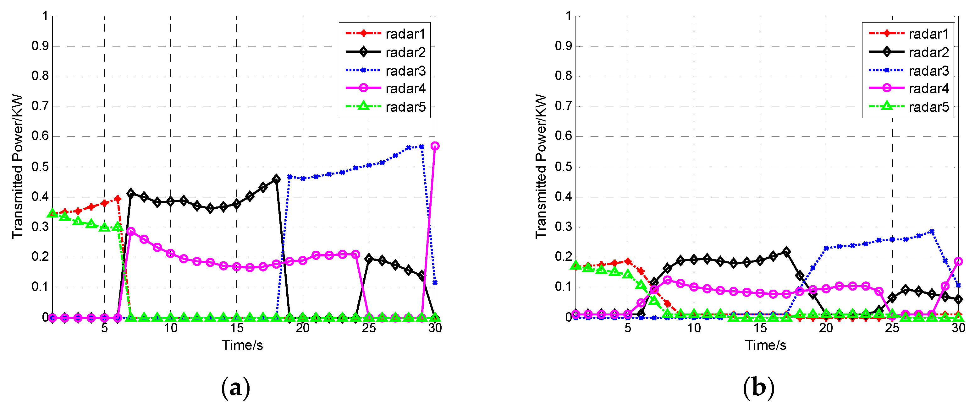
For simplicity, set , , and . The SNR of the radar network, which can guarantee a certain tracking performance of radar network, is set as 13 dB, and the maximum detection range can be calculated according to the equation of radar network. The maximum MMSE threshold can be set as the value of MMSE in the condition that the transmitted power of active radars are equal to 6 KW and the target is located at the maximum detection range. Therefore, it can be calculated that in the case of single radar assigned to each target and in the case of two radars assigned to each target. Figure 3a illustrates the results of target assignment in the case of single radar assigned to each target. Figure 3b illustrates the results of target assignment in the case of two radars assigned to each target.
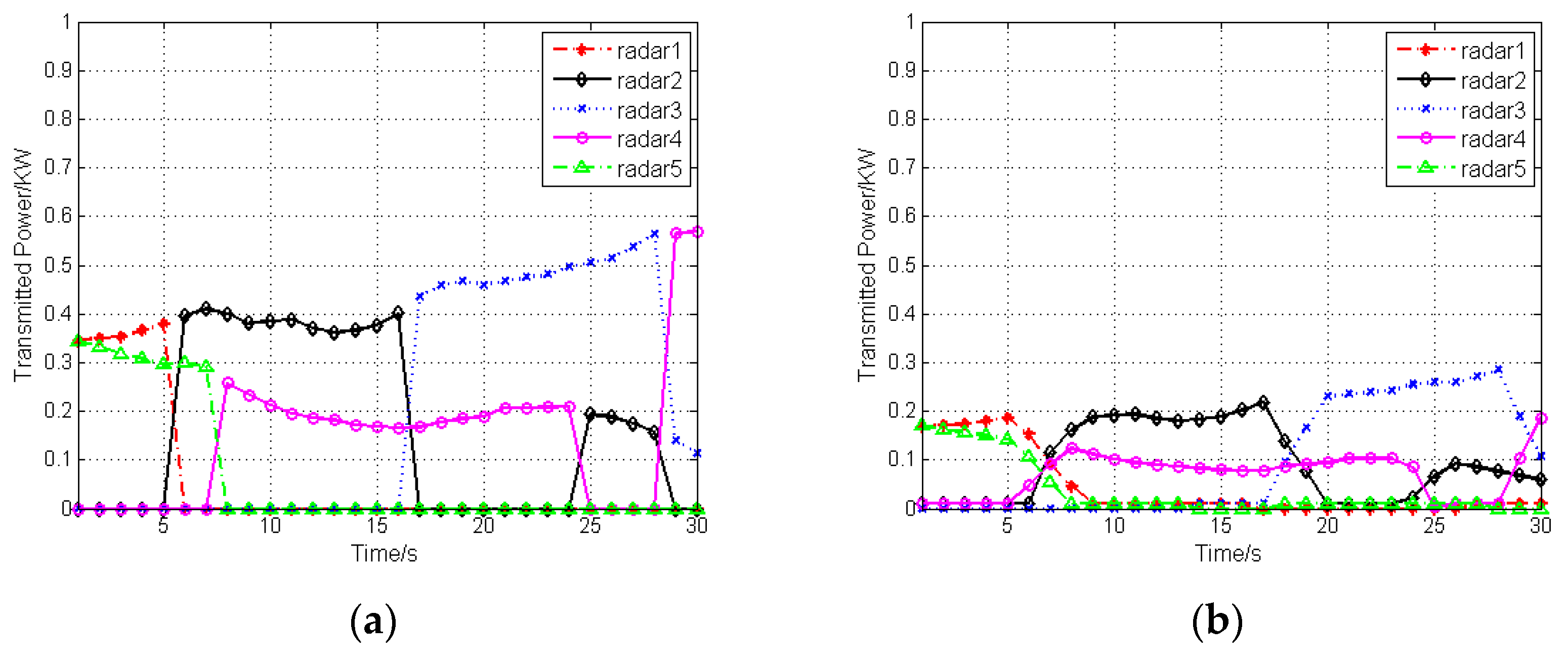
It can be seen from Figure 3 that during the tracking process, with the target movement, radars that are closest to the target are assigned as active radars to track this target. Figure 4a illustrates the results of power allocation in the case of single radar assigned to each target. Figure 4b illustrates the results of power allocation in the case of two radars assigned to each target.
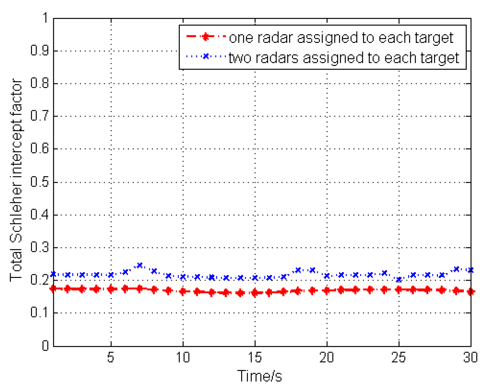
The results of Figure 4 demonstrate that a significant reduction of the transmitted power of radars in the radar network can be achieved after target assignment and power allocation. In order to analyze the LPI performance of radar network after target assignment and power allocation, the total Schleher intercept factor of radar network should be calculated based on the optimum transmitted power. Figure 5 depicts the comparison of the total Schleher intercept factor of radar network between the case of single radar assigned to each target and the case of two radars assigned to each target.
The results of Figure 5 prove that the case of single radar assigned to each target can achieve a smaller total Schleher intercept factor for the radar network than the case of two radars assigned to each target. In traditional radar networks, each radar has a constant transmitted power of 6 KW. Compared to the total Schleher intercept factor of traditional radar network, which is equal to 5, a significant reduction of Schleher intercept factor can be achieved by adopting the LPI optimization algorithm of this paper in both cases. That is, the LPI performance of radar network can be effectively improved in both cases compared with a traditional radar network.
In order to evaluate the effect of radar signal bandwidth on the results of target assignment, we then expand our simulation while considering the second radar signal bandwidth model as follows:
Figure 6a illustrates the effect of the radar signal bandwidth on the target assignment results in the case of single radar assigned to each target. Figure 6b illustrates the effect of the radar signal bandwidth on the target assignment results in the case of two radars assigned to each target.
Figure 7a illustrates the effect of the radar signal bandwidth on the power allocation results in the case of a single radar assigned to each target. Figure 7b illustrates the effect of the radar signal bandwidth on the power allocation results in the case of two radars assigned to each target.
In the second radar signal bandwidth model, the radar signal bandwidth decreased from radar 5 to radar 1. As demonstrated in Figure 6, compare to the uniform bandwidth model, more targets are assigned to radar 3, radar 4, and radar 5. In other words, more targets are assigned to the radars with wide bandwidth. The results of power allocation with the second radar signal bandwidth model have small differences with the uniform bandwidth model as shown in Figure 7.
In reference [23], we proposed a LPI optimization criterion based on the predefined mutual information (MI) threshold. We take the case of a single radar assigned to each target as an example to compare the effects of the criterion of MMSE threshold that this paper proposed with the effects of the criterion of MI threshold reference [23] proposed. The minimum MI threshold can be set as , which is equal to the value of MI in the same condition of MMSE threshold. Figure 8 depicts the results of power allocation by employing the MMSE estimation criterion and the MI criterion.
Figure 9 illustrates the total Schleher intercept factor of radar network by employing the MMSE estimation criterion and the MI criterion.
Figure 9 implies that, from time index to , the total Schleher intercept factor of the radar network by employing the MMSE estimation criterion is smaller than the MI criterion. From time index to , the MI criterion can get a smaller Schleher intercept factor. It can be concluded that the MMSE estimation criterion can get better a LPI optimization result when targets have a closer distance with the center of the radar network and vice versa. In other words, the difference between the results of the MMSE estimation criterion and the MI criterion depend on the geometrical arrangement of the radar network and the distance between targets and the radar network.
7. Conclusions
An LPI optimization framework with target assignment and power allocation for multiple targets tracking in a radar network system is proposed in this paper based on MMSE estimation. The basis of this framework is to use the optimization algorithm to minimize the total Schleher intercept factor of the radar network under a predetermined MMSE threshold in order to improve the LPI performance of the radar network. For each target, assign a suitable subset of radars with a minimum Schleher intercept factor under the constraint of the MMSE threshold. The resulting optimization problem has been investigated in two cases: single radar assigned to each target and two radars assigned to each target. Simulation results demonstrate that the LPI performance of the radar network with an optimization framework outperforms the traditional radar network counterpart in both cases. Results under the second radar signal bandwidth demonstrate that more targets are assigned to the radars that have wide radar signal bandwidth. In addition, the optimization results of MMSE estimation criterion this paper proposed exhibit greater LPI performance compared with the results of MI criterion that our previous work proposed when targets have closer distance with the center of the radar network. The optimization results of MI criterion have greater LPI performance when targets are farther from the center of radar network. The simulation results show that both MMSE estimation criterion and MI criterion can effectively reduce the total Schleher intercept factor of radar network. The results also show that the difference between MMSE estimation criterion and MI criterion depend on the geometrical arrangement of radar network and the distance between targets and radar network. The MMSE-based optimization algorithm this paper proposed can also be used in multistatic radar. In future work, we will focus our research on the design of radar signal parameters, such as pulse width (PW) and pulse repetition interval (PRI), in order to decrease the probability of classification and identification in threat systems.
Acknowledgments
This work is supported by the National Natural Science Foundation of China (Grant No. 61371170, No. 61671239), the Fundamental Research Funds for the Central Universities (Grant No. NP2015404, No. NS2016038,No. NS2016043), the Natural Science Fund for Colleges and Universities in Jiangsu Province (No. 15KJB510015), the Aeronautical Science Foundation of China (Grant No. 20152052028), the Funding of Jiangsu Innovation Program for Graduate Education (CXLX12_0155) and Key Laboratory of Radar Imaging and Microwave Photonics (Nanjing Univ. Aeronaut. Astronaut.), Ministry of Education, Nanjing University of Aeronautics and Astronautics, Nanjing 211106, China.
Author Contributions
The work was conducted under the cooperation of all authors. Ji She and Jianjiang Zhou designed the LPI optimization framework; Ji She, Fei Wang, and Hailin Li solved the optimization problem; Jianjiang Zhou verified the results; Ji She wrote the paper and all of the authors reviewed the manuscript. All authors have read and approved the final manuscript.
Conflicts of Interest
The authors declare no conflict of interest.
References
- Lynch, D.A., Jr. Introduction to RF Stealth; SciTech Publishing: Richmond, TX, USA, 2004. [Google Scholar]
- Dudczyk, J. Radar emission sources identification based on hierarchical agglomerative clustering for large data sets. J. Sens. 2016. [Google Scholar] [CrossRef]
- Dudczyk, J. A method of feature selection in the aspect of specific identification of radar signals. Bull. Pol. Acad. Sci. Tech. Sci. 2017, 65, 113–119. [Google Scholar] [CrossRef]
- Dudczyk, J.; Kawalec, A. Adaptive forming of the beam pattern of microstrip antenna with the use of an artificial neural network. Int. J. Antennas Propag. 2012. [Google Scholar] [CrossRef]
- Haimovich, A.M.; Blum, R.S.; Cimini, L.J. MIMO radar with widely separated antennas. IEEE Signal Process. Mag. 2008, 25, 116–129. [Google Scholar] [CrossRef]
- Li, J.; Stoica, P. MIMO radar with colocated antennas. IEEE Signal Process. Mag. 2007, 24, 106–114. [Google Scholar] [CrossRef]
- Teng, Y.; Griffiths, H.D.; Baker, C.J. Netted radar sensitivity and ambiguity. IET Radar Sonar Nav. 2007, 1, 479–486. [Google Scholar] [CrossRef]
- Xu, L.; Li, J.; Stoica, P. Target detection and parameter estimation for MIMO radar systems. IEEE Trans. Aerosp. Electron. Syst. 2008, 44, 927–939. [Google Scholar]
- Godrich, H.; Haimovich, A.M.; Blum, R.S. Target localization accuracy gain in MIMO radar based system. IEEE Trans. Inf. Theory 2010, 56, 2783–2803. [Google Scholar] [CrossRef]
- Gorji, A.A.; Tharmarasa, R.; Blair, W.D.; Kirubarajan, T. Multiple unresolved target localization and tracking using collocated MIMO radars. IEEE Trans. Aerosp. Electron. Syst. 2012, 48, 2498–2517. [Google Scholar] [CrossRef]
- Yang, Y.; Blum, R.S. MIMO radar waveform design based on mutual information and minimum mean-square error estimation. IEEE Trans. Aerosp. Electron. Syst. 2007, 43, 330–343. [Google Scholar] [CrossRef]
- Yan, J.K.; Jiu, B.; Liu, H.W. Prior knowledge based simultaneous multibeam power allocation algorithm for cognitive multiple targets tracking in clutter. IEEE Trans. Signal Process. 2015, 63, 512–527. [Google Scholar] [CrossRef]
- Godrich, H.; Chiriac, V.M.; Haimovich, A.M.; Blum, R.S. Target tracking in MIMO radar systems: Techniques and performance analysis. In Proceedings of the IEEE Radar Conference, Washington, DC, USA, 10–14 May 2010. [Google Scholar]
- Wang, F.; Li, H.; Xia, W.; Zhou, J. LPI Airborne Radar Signal Processing Technology; Science Press: Beijing, China, 2015. (In Chinese) [Google Scholar]
- Chen, J.; Wang, F.; Zhou, J.J. Information content based optimal radar waveform design: LPI’s purpose. Entropy 2017, 19, 210. [Google Scholar] [CrossRef]
- Godrich, H.; Petropulu, A.P.; Poor, H.V. Power allocation strategies for target localization in distributed multiple-radar architectures. IEEE Trans. Signal Process. 2011, 59, 3226–3240. [Google Scholar] [CrossRef]
- Shi, C.G.; Wang, F.; Zhou, J.J. LPI based resource management for target tracking in distributed radar network. In Proceedings of the IEEE Radar Conference, Philadelphia, PA, USA, 2–6 May 2016. [Google Scholar]
- Zhang, Z.K.; Zhu, J.H.; Tian, Y.B.; Li, H.L. Novel sensor selection strategy for LPI based on an improved IMMPF tracking method. J. Syst. Eng. Electron. 2014, 25, 1004–1010. [Google Scholar] [CrossRef]
- Yan, J.K.; Liu, H.W.; Jiu, B.; Chen, B. Simultaneous multibeam resource allocation scheme for multiple target tracking. IEEE Trans. Signal Process. 2015, 63, 3110–3122. [Google Scholar] [CrossRef]
- Yan, J.K.; Liu, H.W.; Pu, W.Q.; Zhou, S.H. Joint beam selection and power allocation for multiple target tracking in netted colocated MIMO radar system. IEEE Trans. Signal Process. 2016, 64, 6417–6427. [Google Scholar] [CrossRef]
- Godrich, H.; Petropulu, A.P.; Poor, H.V. Cluster allocation schemes for target tracking in multiple radar architecture. In Proceedings of the Forty Fifth Asilomar Conference on Signals, Systems and Computers, Pacific Grove, CA, USA, 6–9 November 2011. [Google Scholar]
- Andargoli, S.M.H.; Malekzadeh, J. Target assignment and power allocation for LPI radar networks. In Proceedings of the International Symposium on Artificial Intelligence and Signal Processing, Mashhad, Iran, 3–5 March 2015. [Google Scholar]
- She, J.; Wang, F.; Zhou, J. A novel sensor selection and power allocation algorithm for multiple-target tracking in an LPI radar network. Sensors 2016, 16, 2193. [Google Scholar] [CrossRef] [PubMed]
- Schleher, D.C. LPI radar: Fact or fiction. IEEE Aerosp. Electron. Syst. Mag. 2006, 21, 3–6. [Google Scholar] [CrossRef]
- Lewandowski, W.; Azoubib, J.; Klepczynski, W.J. GPS: Primary tool for time transfer. Proc. IEEE 1999, 87, 163–172. [Google Scholar] [CrossRef]
- Song, X.F.; Peter, W.; Zhou, S.L. Optimal power allocation for MIMO radars with heterogeneous propagation losses. In Proceedings of the IEEE International Conference on Acoustics, Speech and Signal Processing, Kyoto, Japan, 25–30 March 2012. [Google Scholar]
- Liu, Z.; Zhao, R.L.; Liu, Y.F.; Zhang, Z.J. Performance analysis on MIMO radar waveform based on mutual information and minimum mean-square error estimation. In Proceedings of the IET International Radar Conference, Guilin, China, 20–22 April 2009. [Google Scholar]
- Poor, H.V. An Introduction to Signal Detection and Estimation, 2nd ed.; Springer: New York, NY, USA, 1994. [Google Scholar]
- Cover, T.M.; Gamal, A. An information-theoretic proof of Hadamard’s inequality. IEEE Trans. Inf. Theory 1983, 29, 930–931. [Google Scholar] [CrossRef]
- Boyd, S.; Vandenberghe, L. Convex Optimization; Cambridge University Press: Cambridge, UK, 2004. [Google Scholar]
- Schrijver, A. Combinatorial Optimization: Polyhedra and Efficiency; Springer: Berlin, Germany, 2003. [Google Scholar]
- Streetly, M. Jane’s Radar and Electronic Warfare Systems: 2008–2009; Jane’s Information Group: Coulsdon, UK, 2008. [Google Scholar]
- Gustafsson, F. Particle filter theory and practice with positioning applications. IEEE Aerosp. Electron. Syst. Mag. 2010, 25, 53–82. [Google Scholar] [CrossRef]
Figure 1.
The geometry of radar network, target, and intercept receiver.
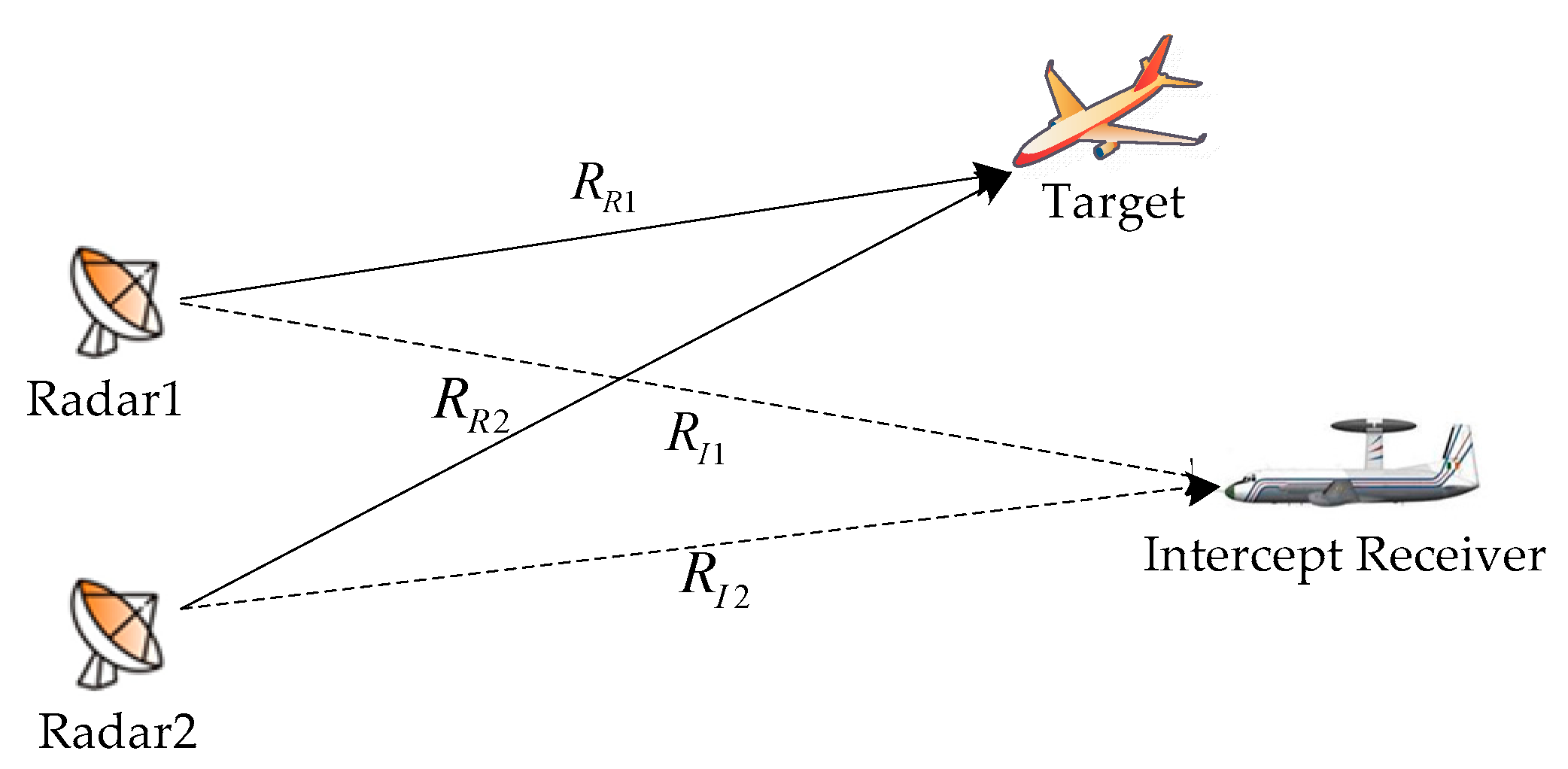
Figure 2.
Target trajectories and the radar network.
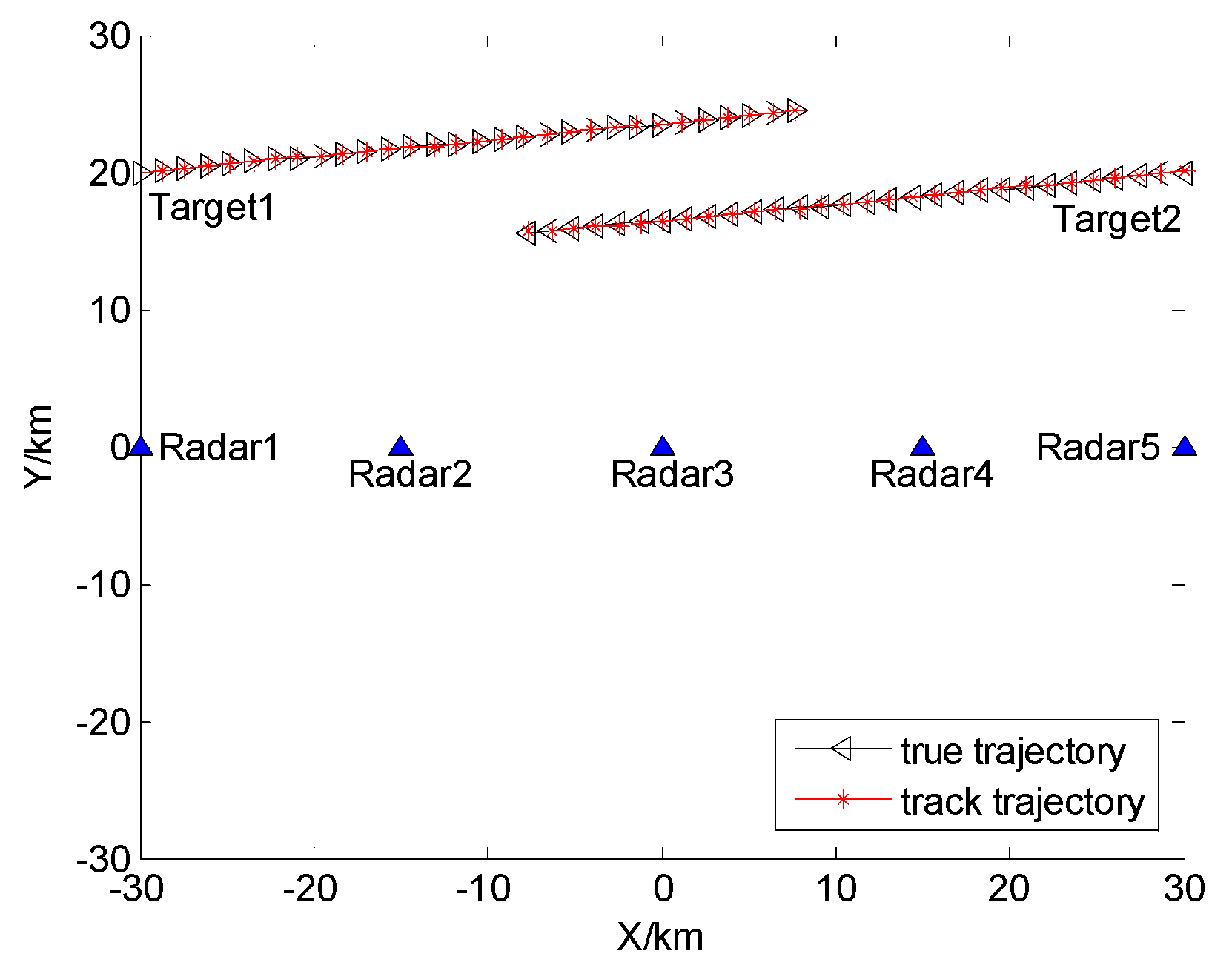
Figure 3.
Target assignment results: (a) Single radar assigned to each target; (b) Two radars assigned to each target.
Figure 3.
Target assignment results: (a) Single radar assigned to each target; (b) Two radars assigned to each target.
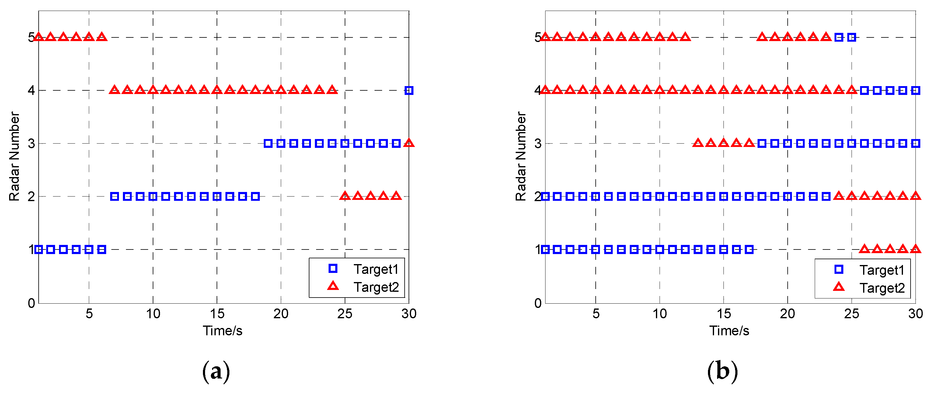
Figure 4.
Power allocation results: (a) Single radar assigned to each target; (b) Two radars assigned to each target.
Figure 4.
Power allocation results: (a) Single radar assigned to each target; (b) Two radars assigned to each target.

Figure 5.
Total Schleher intercept factor in two cases.

Figure 6.
The target assignment results: (a) The second bandwidth model, a single radar assigned to each target; (b) The second bandwidth model, two radars assigned to each target.
Figure 6.
The target assignment results: (a) The second bandwidth model, a single radar assigned to each target; (b) The second bandwidth model, two radars assigned to each target.
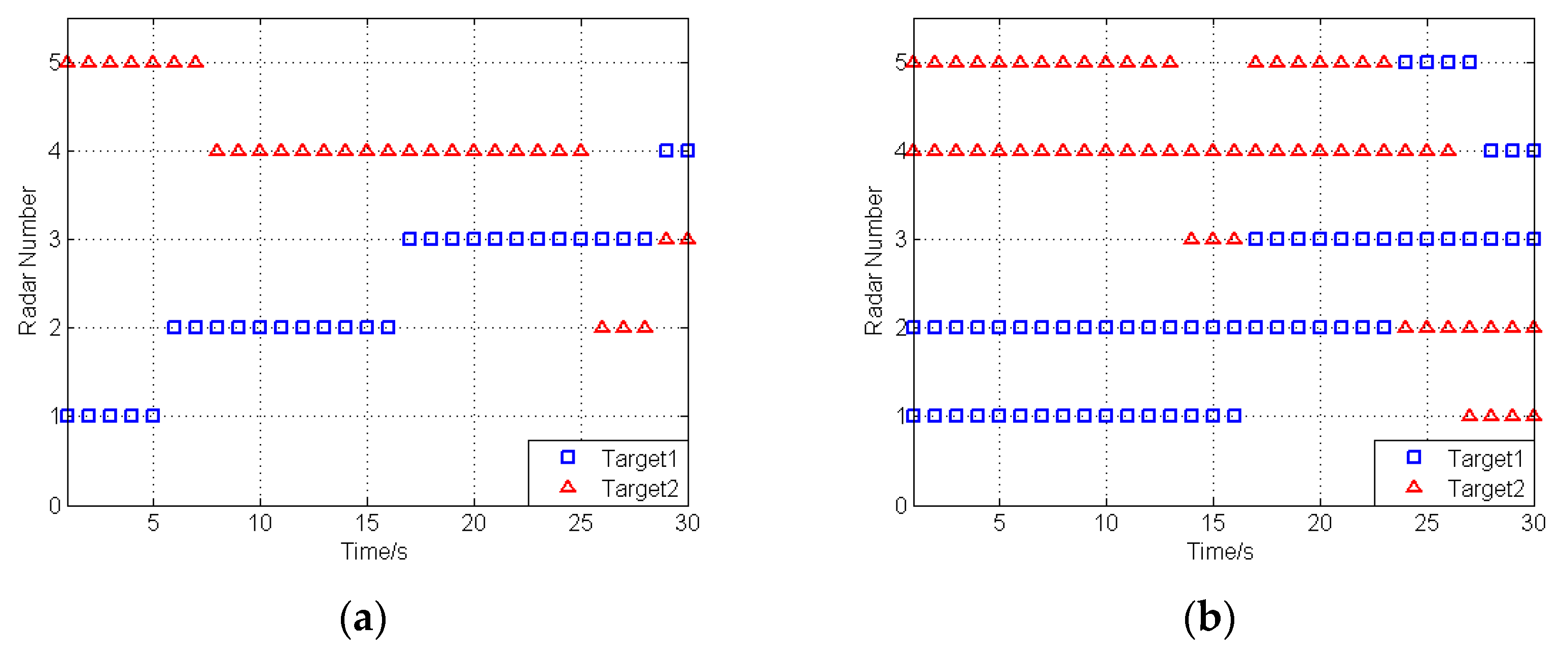
Figure 7.
Power allocation results: (a) The second bandwidth model, a single radar assigned to each target; (b) The second bandwidth model, two radars assigned to each target.
Figure 7.
Power allocation results: (a) The second bandwidth model, a single radar assigned to each target; (b) The second bandwidth model, two radars assigned to each target.

Figure 8.
The results of power allocation by employing the minimum mean-square error (MMSE) estimation criterion and the mutual information (MI) criterion.
Figure 8.
The results of power allocation by employing the minimum mean-square error (MMSE) estimation criterion and the mutual information (MI) criterion.
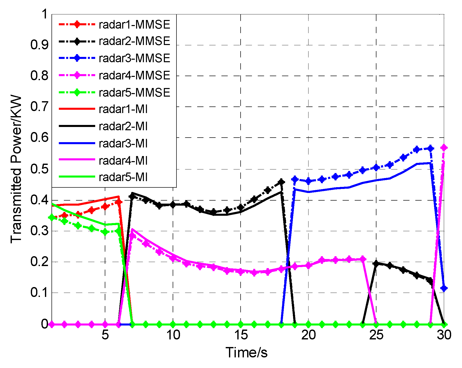
Figure 9.
Total Schleher intercept factor by employing the MMSE estimation criterion and the MI criterion.
Figure 9.
Total Schleher intercept factor by employing the MMSE estimation criterion and the MI criterion.


Table 1.
Minimum Schleher intercept factor matrix.
| Minimum Schleher Intercept Factor | Targets | ||||
|---|---|---|---|---|---|
| ... | |||||
| Radars | … | ||||
| … | |||||
| ⋮ | ⋮ | ⋮ | ⋮ | ||
| … | |||||
Table 2.
Minimum sum of Schleher intercept factor matrix of two-radar combinations.
| Minimum Sum of Schleher Intercept Factor | Targets | ||||
|---|---|---|---|---|---|
| ... | |||||
| Radars | … | ||||
| … | |||||
| ⋮ | ⋮ | ⋮ | ⋮ | ||
| … | |||||
Table 3.
The parameters of radars.
| Parameters | Value |
|---|---|
| Maximum Peak Power | 6 KW |
| Transmitted Antenna Gain | 30 dB |
| Received Antenna Gain | 30 dB |
| Bandwidth | 1 MHz |
Table 4.
The parameters of each target.
| Target Index | 1 | 2 |
|---|---|---|
| Initial Position Coordinate (km) | (−30, 20) | (30, 20) |
| Velocity (km/s) | (1.3, 0.15) | (−1.3, −0.15) |
© 2017 by the authors. Licensee MDPI, Basel, Switzerland. This article is an open access article distributed under the terms and conditions of the Creative Commons Attribution (CC BY) license (http://creativecommons.org/licenses/by/4.0/).
Share and Cite
MDPI and ACS Style
She, J.; Zhou, J.; Wang, F.; Li, H. LPI Optimization Framework for Radar Network Based on Minimum Mean-Square Error Estimation. Entropy 2017, 19, 397. https://doi.org/10.3390/e19080397
AMA Style
She J, Zhou J, Wang F, Li H. LPI Optimization Framework for Radar Network Based on Minimum Mean-Square Error Estimation. Entropy. 2017; 19(8):397. https://doi.org/10.3390/e19080397
Chicago/Turabian StyleShe, Ji, Jianjiang Zhou, Fei Wang, and Hailin Li. 2017. "LPI Optimization Framework for Radar Network Based on Minimum Mean-Square Error Estimation" Entropy 19, no. 8: 397. https://doi.org/10.3390/e19080397
Note that from the first issue of 2016, this journal uses article numbers instead of page numbers. See further details here.