Self-Organized Supercriticality and Oscillations in Networks of Stochastic Spiking Neurons

Abstract

Networks of stochastic spiking neurons are interesting models in the area of theoretical neuroscience, presenting both continuous and discontinuous phase transitions. Here, we study fully-connected networks analytically, numerically and by computational simulations. The neurons have dynamic gains that enable the network to converge to a stationary slightly supercritical state (self-organized supercriticality (SOSC)) in the presence of the continuous transition. We show that SOSC, which presents power laws for neuronal avalanches plus some large events, is robust as a function of the main parameter of the neuronal gain dynamics. We discuss the possible applications of the idea of SOSC to biological phenomena like epilepsy and Dragon-king avalanches. We also find that neuronal gains can produce collective oscillations that coexist with neuronal avalanches.

1. Introduction

Neuronal network models are extended dynamical systems that may present different collective behaviors or phases characterized by order parameters. The separation regions between phases can be described as bifurcations in the order parameters or phase transitions. In several models of neuronal activity, the relevant phase change is a continuous transition from an absorbing silent state to an active state [1,2,3]. In such a continuous transition, we have a critical point (in general, a critical surface) where concepts of universality classes and critical exponents (among others) are valid. At criticality, we observe avalanches of activity described by power laws for their size and duration. Furthermore, the avalanche profile shows fractal scaling. Since the landmark findings of Beggs and Plenz in 2003 [2], these behaviors have been reported also in biological networks; see the reviews [4,5,6,7].

The motivation for the idea that criticality is important to understand neuronal activity is not only empirical. Several works have shown that there are advantages for a network to operate at the critical state [3,8,9,10]. However, it is not clear how biological networks tune themselves to the critical region.

An important idea discussed in several papers is that, since criticality depends on the strength of the synapses (links) between the neurons, a homeostatic mechanism for dynamic synapses tunes the network toward the critical region. There are two main paradigms: self-organization of Hebbian synapses [11,12,13,14,15,16] and self-organization of dynamic synapses [17,18,19,20,21] following Tsodyks and Markran [22,23]. With these synaptic mechanisms, it is possible to achieve, or at least to approximate, a self-organized critical (SOC) state.

With a different approach, we have shown recently that dynamic neuronal gains, biophysically linked to firing-dependent excitability of the axonal initial segment (AIS) [24,25,26,27], can also lead to self-organized criticality [28]. This new mechanism is simpler than dynamic synapses because, for biological networks with N neurons, we have of the order of ${10}^{4}N$ synapses [29], and thus ${10}^{4}N$ dynamic equations, but only N equations for the neuronal gains.

It has also been observed in Brochini et al. [28] that, for achieving exact SOC, all papers in the literature used a time scale $\tau$ for synaptic recovery proportional to N, with $N\to \infty$. The use of this non-local information (N), and a diverging recovery time $\tau$, is not plausible biologically. A similar time scale $\tau$ is present in the neuronal gain recovery. When we use a biological range for $\tau$ that does not scale with N, we observe that the network turns out (slightly) supercritical, a phenomenon that we called self-organized supercriticality (SOSC). That is, both dynamic synapses and dynamic gains with fixed $\tau$, which seems to be the reasonable biological assumption, present SOSC instead of SOC.

Here, we report for the first time an extensive study of the neuronal gain mechanism and SOSC. First, we present new mean-field results for phase transitions in a fully-connected model of integrate-and-fire stochastic neurons with fixed gains. We find both continuous and discontinuous phase transitions. Then, we introduce a simplified gain dynamics depending only on the $\tau$ parameter, which also has a simple mean-field solution in the case of the continuous transition and presents SOSC. We compare this solution with extensive simulations for different system sizes N and values for $\tau$. Surprisingly, we found collective oscillations produced by the gain dynamics that coexist with neuronal avalanches.

2. The Model

We consider a fully-connected network composed of $i=1,\dots ,N$ discrete-time stochastic neurons [28,30,31,32,33]. The synapses transmit signals from some presynaptic neuron j to a postsynaptic neuron i with synaptic strength $W_{ij}$. The Boolean variable $X_i\left[t\right]\in \left\{0,1\right\}$ denotes whether neuron i fired between t and $t+1$, and $V_i\left[t\right]$ corresponds to its membrane potential at time t. Firing $X_i[t+1]=1$ occurs with probability $\mathsf{\Phi }\left(V_i\left[t\right]\right)$, which is called the firing function [32,33,34,35,36,37].

If a presynaptic neuron j fires at discrete time t, then $X_j\left[t\right]=1$. This event increments by $W_{ij}$ the potential of every postsynaptic neuron i that has not fired at time t. The potential of a non-firing neuron may also integrate an external stimulus $I_i\left[t\right]$. Apart from these increments, the potential of a non-firing neuron decays at each time step towards zero by a factor $\mu \in [0,1]$, which models the effect of a current leakage.

The neuron membrane potentials evolve as:

$$V_i[t+1]=\left\{\begin{array}{ccc}{\displaystyle 0}\hfill & & \mathrm{if}{X}_i\left[t\right]=1,\hfill \\ {\displaystyle \mu V_i\left[t\right]+I_i\left[t\right]+\frac{1}{N}\sum _{j=1}^N{W}_{ij}{X}_j\left[t\right]}\hfill & & \mathrm{if}{X}_i\left[t\right]=0.\hfill \end{array}\right.$$

(1)

This is a special case of the general model from [32] with the filter function $g(t-t_s)={\mu }^{t-t_s}$, where $t_s$ is the time of the last firing of neuron i [28]. In contrast to standard integrate-and-fire (IF) neurons, the firing is not deterministic above a threshold, but stochastic. We also have $X_i[t+1]=0$ if $X_i\left[t\right]=1$ (refractory period of one time step).

The firing function $0\le \mathsf{\Phi }\left(V\right)\le 1$ is sigmoidal, that is monotonically increasing. We also assume that $\mathsf{\Phi }\left(V\right)$ is zero up to some threshold potential $V_T$. If $\mathsf{\Phi }$ is the shifted Heaviside step function $\mathsf{\Phi }\left(V\right)=\mathsf{\Theta }(V-V_T)$, we have a deterministic discrete-time leaky integrate-and-fire (LIF) neuron. Any other choice for $\mathsf{\Phi }\left(V\right)$ gives a stochastic neuron.

In Brochini et al. [28], we have studied a linear saturating function with neuronal gain $\mathsf{\Gamma }$ similar to that used in [33]. Here, we study the so-called rational function that does not have a saturating potential; see Figure 1a:

$$\mathsf{\Phi }\left(V\right)=\frac{\mathsf{\Gamma }(V-V_T)}{1+\mathsf{\Gamma }(V-V_T)}\mathsf{\Theta }(V-V_T).$$

(2)

Notice that we recover the deterministic LIF model $\mathsf{\Phi }\left(V\right)=\mathsf{\Theta }(V-V_T)$ when $\mathsf{\Gamma }\to \infty$. The use of the rational instead of the linear saturating function is convenient and gives some theoretical advantages, for example to avoid the anomalous cycles-two observed in [28].

3. Mean-Field Calculations

The network’s activity is measured by the fraction $\rho \left[t\right]$ of firing neurons (or density of active sites):

$$\rho \left[t\right]=\frac{1}{N}\sum _{j=1}^N{X}_j\left[t\right].$$

(3)

The density of active neurons $\rho \left[t\right]$ can be computed from the probability density $p\left[t\right]\left(V\right)$ of potentials at time t:

$$\begin{array}{c}\hfill \rho \left[t\right]={\int }_{-\infty }^{\infty }\mathsf{\Phi }\left(V\right)p\left[t\right]\left(V\right)dV,\end{array}$$

(4)

where $p\left[t\right]\left(V\right)dV$ is the fraction of neurons with potential in the range $[V,V+dV]$ at time t.

Neurons that fire between t and $t+1$ have their potential reset to zero. They contribute to $p[t+1]\left(V\right)$ a Dirac impulse at potential $V=0$, with amplitude $\rho \left[t\right]$ given by Equation (4). The potentials of all neurons also evolve according to Equation (1). This process modifies $p\left[t\right]\left(V\right)$ also for $V\ne 0$.

In the mean-field limit, we assume that the synaptic weights $W_{ij}$ follow a distribution with average $W=〈W_{ij}〉$ and finite variance. By disregarding correlations, the term in Equation (1) corresponding to the sum of all presynaptic inputs simplifies to $W\rho \left[t\right]$.

If the external input is constant, $I_i\left[t\right]=I$, a stationary state is achieved, which depends only on the average synaptic weight W, the leakage parameter $\mu$ and the parameters that define the function $\mathsf{\Phi }\left(V\right)$, that is $\mathsf{\Gamma }$ and $V_T$. In Brochini et al. [28], it is shown that the stationary $p\left(V\right)$ is composed of delta peaks with height ${\eta }_k$ situated at voltages $U_k$ given by:

$$\begin{array}{ccc}\hfill U_0& =& 0,\hfill \end{array}$$

(5)

$$\begin{array}{ccc}\hfill U_k& =& \mu U_{k-1}+I+W\rho ,\hfill \end{array}$$

(6)

$$\begin{array}{ccc}\hfill {\eta }_k& =& \left(1-\mathsf{\Phi }\left(U_{k-1}\right)\right){\eta }_{k-1},\hfill \end{array}$$

(7)

$$\begin{array}{ccc}\hfill \rho & =& {\eta }_0=\sum _{k=0}^{\infty }\mathsf{\Phi }\left(U_k\right){\eta }_k,\hfill \end{array}$$

(8)

for all $k\ge 1$. Here, $U_k$ corresponds to the potential value of the population of neurons that have firing age k. The firing age is the amount of time steps since the neuron fired for the last time. The normalization condition ${\sum }_{k=0}^{\infty }{\eta }_k=1$ must be included explicitly. Equations (6)–(8) can be solved numerically for any firing function $\mathsf{\Phi }$, so this result is very general.

4. Results

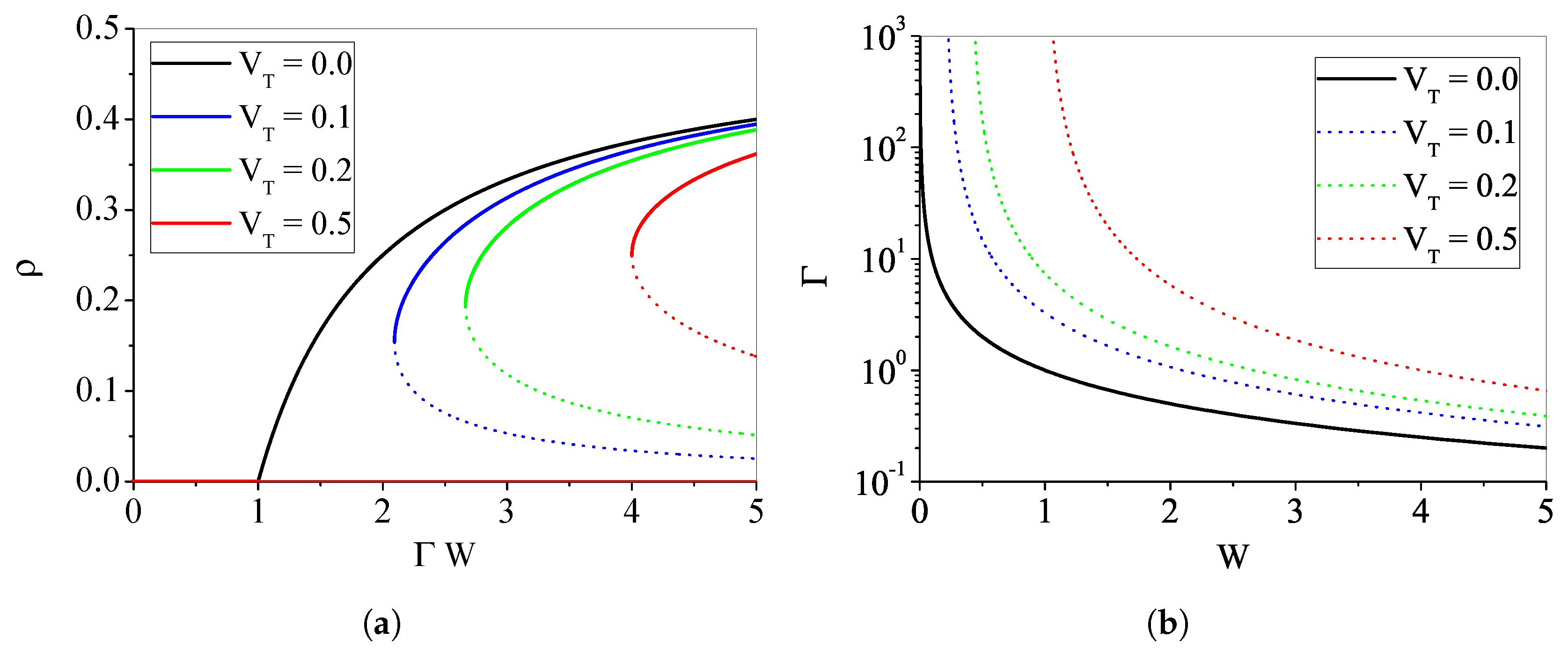
4.1. Phase Transitions for the Rational $\Phi \left(V\right)$

In terms of non-equilibrium statistical physics, $\rho$ is the order parameter; I is a uniform external field; and $\mathsf{\Gamma }$ and W are the main control parameters. The activity $\rho$ also depends on $V_T$ and $\mu$.

4.1.1. The Case with $\mu >0,I=0,V_T=0$

By using Equations (5)–(8), we obtain numerically $\rho (W,\mathsf{\Gamma })$ for several values of $\mu >0$, for the case with $I=0,V_T=0$ (Figure 1b). Only the first 100 peaks $(U_k,{\eta }_k)$ were considered, since, for the given $\mu$ and $\mathsf{\Phi }$, there was no significant probability density beyond that point. The same numerical method can be used for studying the cases $I\ne 0,V_T\ne 0$.

We also obtained an analytic approximation (see Appendix) for small $\rho$:

$$\rho \approx \left(\frac{1}{2+\mu +{\mu }^2/(1-\mu )}\right)\frac{\mathsf{\Gamma }-{\mathsf{\Gamma }}_C}{\mathsf{\Gamma }}\propto {\Delta }_{\mathsf{\Gamma }}^{\beta },$$

(9)

where ${\mathsf{\Gamma }}_C=(1-\mu )/W$ defines the critical line and ${\Delta }_{\mathsf{\Gamma }}=(\mathsf{\Gamma }-{\mathsf{\Gamma }}_C)/\mathsf{\Gamma }$ is the reduced control parameter. Therefore, the critical exponent for the order parameter near criticality is $\beta =1$, characteristic of the mean-field directed percolation (DP) universality class [38]. We also compare Equation (9) with the numerical results for $\rho (\mathsf{\Gamma },\mu )$ in Figure 1c.

4.1.2. Analytic Results for $\mu =0$

In the case $\mu =0$, it is possible to do a simple mean-field analysis valid for $N\to \infty$. This case is illustrative because it presents all phase transitions that occur with $\mu >0$.

When $\mu =0$ and $I_i\left[t\right]=I$ (uniform constant input), the stationary density $p\left(V\right)$ consists of only two Dirac peaks at potentials $U_0=0$ and $U_1=I+W\rho$. Equation (8) simplifies to:

$$\rho =\rho \mathsf{\Phi }\left(0\right)+(1-\rho )\mathsf{\Phi }(I+W\rho ),$$

(10)

since ${\eta }_0=\rho$ and ${\eta }_1=1-\rho$.

By inserting the function Equation (2) in Equation (10) and remembering that $\mathsf{\Phi }\left(0\right)=0$, we get:

$$2\mathsf{\Gamma }W{\rho }^2-(\mathsf{\Gamma }W+2\mathsf{\Gamma }(V_T-I)-1)\rho +\mathsf{\Gamma }(V_T-I)=0,$$

(11)

with solutions:

$$\begin{array}{ccc}\hfill {\rho }^{\pm }& =& \frac{\mathsf{\Gamma }(W+2V_T-2I)-1\pm \sqrt{\Delta }}{4\mathsf{\Gamma }W},\hfill \end{array}$$

(12)

$$\begin{array}{ccc}\hfill \Delta & =& {(\mathsf{\Gamma }(W+2V_T-2I)-1)}^2-8{\mathsf{\Gamma }}^{2}W(V_T-I),\hfill \end{array}$$

(13)

4.1.3. The Case with $I=0,V_T=0$: Continuous Transition

For $V_T=I=0$, we have:

$$\begin{array}{ccc}\hfill \rho \left(W\right)& =& \frac{1}{2}{\left(\frac{W-W_C}{W}\right)}^{\beta }=\frac{1}{2}{\left(\frac{\mathsf{\Gamma }-{\mathsf{\Gamma }}_C}{\mathsf{\Gamma }}\right)}^{\beta },\hfill \end{array}$$

(14)

where the phase transition line is:

$${\mathsf{\Gamma }}_C=1/W_C,$$

(15)

and the critical exponent is $\beta =1$. This corresponds to a standard mean-field continuous (second order) absorbing state phase transition (Figure 2a,b with $V_T=I=0$).

4.1.4. The Case with $I<V_T$: Discontinuous Transition

For $I<V_T$, we have discontinuous (first order) phase transitions when $\Delta =0$ (see Equation (13)):

$${\left({\mathsf{\Gamma }}_C{W}_C+2{\mathsf{\Gamma }}_C(V_T-I)-1\right)}^2=8{\mathsf{\Gamma }}_C^2{W}_C(V_T-I),$$

(16)

which, after some algebra, leads to the phase transition lines:

$$\begin{array}{ccc}\hfill {\mathsf{\Gamma }}_C{W}_C& =& {\left(1+\sqrt{2{\mathsf{\Gamma }}_C(V_T-I)}\right)}^2,\hfill \end{array}$$

(17)

$$\begin{array}{ccc}\hfill {\mathsf{\Gamma }}_C& =& \frac{1}{{\left(\sqrt{W_C}-\sqrt{2(V_T-I)}\right)}^2}\hfill \end{array}$$

(18)

which have the correct limit, Equation (15), when $V_T\to 0,I\to 0$. The transition discontinuity is:

$${\rho }_C=\frac{\sqrt{V_T-I}}{\sqrt{2W_C}}=\frac{1}{2}\frac{\sqrt{2{\mathsf{\Gamma }}_C(V_T-I)}}{1+\sqrt{2{\mathsf{\Gamma }}_C(V_T-I)}}.$$

(19)

In Figure 2a, we show examples of the phase transitions, which occur when the unstable point ${\rho }^{-}$ collapses with the stable point ${\rho }^{+}$. It is important to notice that, for any $V_T>0$, the unstable point never touches the absorbing point ${\rho }_0=0$, so the zero solution is always stable. Only for the case $V_T=0$, the solution ${\rho }_0$ looses stability, and ${\rho }^{+}$ is the unique solution above the critical line ${\mathsf{\Gamma }}_C=1/W_C$. Figure 2b gives the phase diagram $\mathsf{\Gamma }\times W$ for some values of $V_T$ with $I=0$; see Equation (18). Finally, we give the phase diagram for the variables $\mathsf{\Gamma }W$ versus $\mathsf{\Gamma }(V-I)$; see Figure 3 and Equation (17).

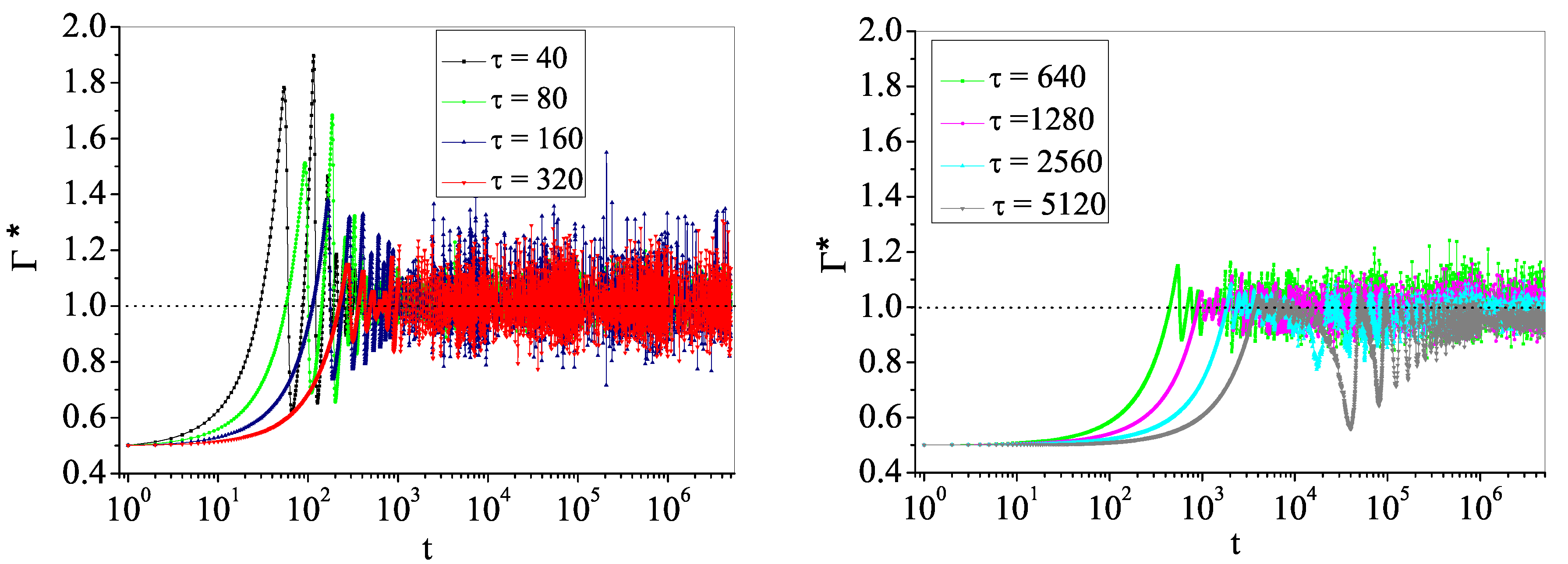
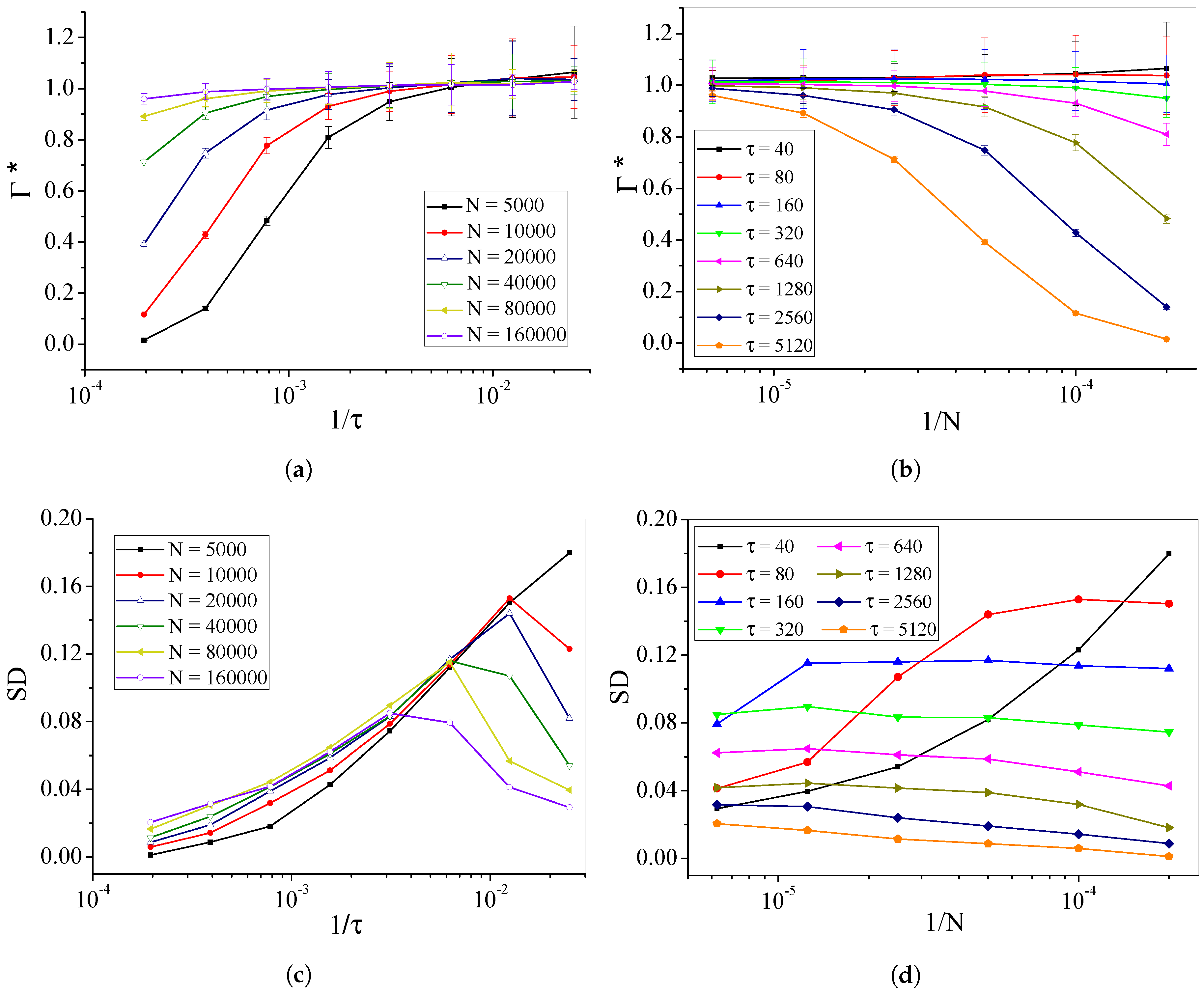
4.2. Self-Organized Supercriticality through Dynamic Gains with $\mu =0$, $I=0$, $V_T=0$

If we fine-tune the model to some point in the critical line ${\mathsf{\Gamma }}_C=1/W$, we can observe perfect neuronal avalanches with size distribution $P_S\left(s\right)\propto s^{-3/2}$ and duration distribution $P_D\left(d\right)\propto d^{-2}$ [28]. As expected, these are mean-field exponents fully compatible with the experimental results [2,6].

This fine-tuning, however, is not plausible biologically. What we need is some homeostatic mechanism that makes the critical region an attractor of some self-organization dynamics. In the literature, a well-studied mechanism is dynamic synapses $W_{ij}\left[t\right]$ [17,18,19]. For example, in discrete time [20,21]:

$$W_{ij}[t+1]=W_{ij}\left[t\right]+\frac{1}{\tau }(A-W_{ij}\left[t\right])-u{W}_{ij}\left[t\right]X_j\left[t\right],$$

(20)

where $\tau$ is a synaptic recovery time, A is an asymptotic value and $u\in [0,1]$ is the fraction of the depletion of neurotransmitter vesicles when the presynaptic neuron fires.

In Brochini et al. [28], we proposed a new self-organization mechanism based on dynamic neuronal gains ${\mathsf{\Gamma }}_i\left[t\right]$ while keeping the synapses $W_{ij}$ fixed [28]. The idea is to create a feedback loop based only on the local activity $X_i\left[t\right]$ of the neuron, reducing the gain when the neuron fires and recovering slowly after that. The biological motivation for dynamic gains is spike frequency adaptation, a well-known phenomenon that depends on the decrease (and recovery) of sodium ion channels’ density at the axon initial segment (AIS) when the neuron fires [25,26].

The dynamics for the neuronal gains studied in [28] has a form similar to that used in [17,19,20,21] for synapses:

$${\mathsf{\Gamma }}_i[t+1]={\mathsf{\Gamma }}_i\left[t\right]+\frac{1}{\tau }(A-{\mathsf{\Gamma }}_i\left[t\right])-u{\mathsf{\Gamma }}_i\left[t\right]X_i\left[t\right].$$

(21)

The advantage of neuronal gains is that now we have only N dynamical equations (notice the term $X_i\left[t\right]$ that refers to the activity of the postsynaptic neuron, not of the presynaptic one as in Equation (20)). For dynamic synapses, we need to simulate $N(N-1)$ equations for the fully-connected graph model and ${10}^{4}N$ for a biologically-realistic network, and this is computationally very costly for large N.

A problem with this dynamics, however, also present in dynamic synapses, is that we have a three-dimensional parameter space ($\tau \in [1,\infty ],A\in [1/W,\infty ],u\in [0,1]$) that must be fully explored to characterize the stationary value ${\mathsf{\Gamma }}^{*}(\tau ,A,u,N)$. Here, we propose a new simplified dynamics with a single free parameter, the gain recovery time $\tau$:

$${\mathsf{\Gamma }}_i[t+1]={\mathsf{\Gamma }}_i\left[t\right]+\frac{1}{\tau }{\mathsf{\Gamma }}_i\left[t\right]-{\mathsf{\Gamma }}_i\left[t\right]X_i\left[t\right]=\left(1+\frac{1}{\tau }-X_i\left[t\right]\right)\mathsf{\Gamma }\left[t\right].$$

(22)

The self-organization mechanism can be viewed in Figure 4. Therefore, we reduce our parametric study to determine the curves ${\mathsf{\Gamma }}^{*}(1/\tau ,1/N)$; see Figure 5a,b. The fluctuations measured by the standard deviation $SD$ of the $\mathsf{\Gamma }\left[t\right]$ time series, after the transient, diminish for increasing $\tau$ (Figure 5c) and probably go to zero for $\tau \to \infty$, in accord with Campos et al. [21]. However, in contrast to this idealized $\tau \to \infty$ limit, as discussed in [19,21], the fluctuations do not converge to zero for finite $\tau$ in the thermodynamic limit $N\to \infty$ (see Figure 5d). This occurs because, for low $\tau$, the adaptation mechanism produces oscillations of $\mathsf{\Gamma }\left[t\right]$ around the value ${\mathsf{\Gamma }}^{*}\left(\tau \right)$.

We can do a mean-field analysis of Equation (22) to find the value ${\mathsf{\Gamma }}^{*}\left(\tau \right)$. Denote the average gain as $\mathsf{\Gamma }\left[t\right]=〈{\mathsf{\Gamma }}_i\left[t\right]〉$. Averaging over the sites, we have:

$$\mathsf{\Gamma }[t+1]=\mathsf{\Gamma }\left[t\right]+\frac{1}{\tau }\mathsf{\Gamma }\left[t\right]-\rho \left[t\right]\mathsf{\Gamma }\left[t\right],$$

(23)

since $\rho \left[t\right]=〈X_i\left[t\right]〉$. In the stationary state, we have $\mathsf{\Gamma }[t+1]=\mathsf{\Gamma }\left[t\right]={\mathsf{\Gamma }}^{*},\rho \left[t\right]={\rho }^{*}$, so:

$$\frac{1}{\tau }{\mathsf{\Gamma }}^{*}={\rho }^{*}{\mathsf{\Gamma }}^{*}.$$

(24)

A solution is ${\mathsf{\Gamma }}^{*}=0$, but this is unstable; see Equation (22). Another solution is obtained by inserting Equation (14), ${\rho }^{*}=({\mathsf{\Gamma }}^{*}-{\mathsf{\Gamma }}_C)/\left(2{\mathsf{\Gamma }}^{*}\right)$, in Equation (24):

$${\mathsf{\Gamma }}^{*}=\frac{{\mathsf{\Gamma }}_C}{1-2/\tau }.$$

(25)

Notice that this is valid only when Equation (14) is valid, that is, for ${\mathsf{\Gamma }}^{*}\ge 1/W$. Furthermore, Equation (25) presumes that ${\rho }^{*}$ is a stable fixed point, which can not be true for some interval of values of $\tau$; see below.

A first order approximation leads to:

$${\mathsf{\Gamma }}^{*}={\mathsf{\Gamma }}_C\left(1+\frac{2}{\tau }\right).$$

(26)

This mean-field calculation shows that, if $\tau \to \infty$, we obtain an exact SOC state ${\mathsf{\Gamma }}^{*}\to {\mathsf{\Gamma }}_C$; or for finite networks, a scaling $\tau =O\left(N^a\right)$ with an exponent $a>0$ would be required, as done previously for dynamic synapses [17,19,20,21]. However, this scaling for $\tau$ cannot be justified biologically.

Therefore, biology requires a finite recovery time $\tau$, which always leads to supercriticality; see Equation (25) or (26). This supercriticality is self-organized in the sense that it is achieved and maintained by the gain dynamics Equation (22). We call this phenomena self-organized supercriticality (SOSC).

The deviation from criticality can be small. For example, if $\tau =1000$ ms (assuming one time step equals 1 ms in the model):

$${\mathsf{\Gamma }}^{*}\approx 1.002{\mathsf{\Gamma }}_C.$$

(27)

Even a more conservative value $\tau =100$ ms gives ${\mathsf{\Gamma }}^{*}\approx 1.02{\mathsf{\Gamma }}_C$. Although not perfect SOC [5], this result is sufficient to explain a power law with exponent $3/2$ for small ($s<1000$) neuronal avalanches plus a supercritical bump (Figure 6).

By using Equation (25) in Equation (14), we also obtain:

$${\rho }^{*}=\frac{1}{\tau }$$

(28)

showing that the network presents supercritical activity for any finite $\tau$. This result, however, is valid only in the infinite size limit. For finite size networks, fluctuations interrupt this constant ${\rho }^{*}=1/\tau$ activity, leading the system to the absorbing state and defining the end of the avalanches.

Simulations reveal that these fixed points $({\mathsf{\Gamma }}^{*},{\rho }^{*})$ correspond only to mean values around which both $\mathsf{\Gamma }\left[t\right]$ and $\rho \left[t\right]$ oscillate; see Figure 7a–c. These global oscillations are unexpected since the model has been devised to produce avalanches, not oscillations. The finite size fluctuations and oscillations drive the network to the absorbing zero state, generating the avalanches. What we see in the histogram of Figure 6 is a combination of power law avalanches in some range plus large events (superavalanches or Dragon-kings due to the $\mathsf{\Gamma }\left[t\right]$ oscillations).

5. Discussion

We examined a network of stochastic spiking neurons with a rational firing function $\mathsf{\Phi }$ that has not been studied previously. We obtained numeric and analytic results that show the presence of continuous and discontinuous absorbing phase transitions. Classic SOC is possible only at the continuous transition, which means that we need to use zero firing thresholds ($V_T=0$). In some sense, this is a kind of fine-tuning of the $\mathsf{\Phi }$ function, but not the usual one where the synaptic strength W and the neuronal gain $\mathsf{\Gamma }$ are the main control parameters.

The presence of a well-behaved absorbing phase transition in the directed percolation class enables the use of a homeostatic mechanism for the neuronal gains that tunes the network to the critical region. The dynamics on the gains is biologically plausible and can be related to a decrease and recovery, due to the neuron activity, of the firing probability at the axon initial segment (AIS) [24]. Our dynamic ${\mathsf{\Gamma }}_i\left[t\right]$ mimics the well-known phenomenon of spike frequency adaptation [25,26] and is a one-parameter simplification of the three-parameter dynamics studied by us in [28].

We observe that this gain dynamics is equivalent to approaching the critical line with fixed W and variable $\mathsf{\Gamma }\left[t\right]$, that is performing vertical movements in Figure 2b. Previous literature approaches the critical point $W_C$ by dynamic [17,18,19,20,21] or Hebbian [11,12,13,14,15,16] synapses. This corresponds to fixing $\mathsf{\Gamma }$ and allowing changes in $W_{ij}\left[t\right]$ along the horizontal axis; see Figure 2b.

The two homeostatic strategies are similar, but we stress that we have only N equations for the gains ${\mathsf{\Gamma }}_i\left[t\right]$ instead of $N(N-1)$ equations for the synapses $W_{ij}\left[t\right]$, so that our approach implies a huge computational advantage. Indeed, previous literature as [14,17] reported system sizes on the range of $N=$ 1000–4000, to be compared to our maximal size of $N=$ 160,000.

We found that the fixed point ${\mathsf{\Gamma }}^{*}$ predicted by a mean-field calculation is not exactly critical, but instead supercritical, and that the distance from criticality depends on the gain recovery time $\tau$. Previous claims about achieving exact SOC by using dynamic synapses are based on the erroneous assumption that we can use a synaptic recovery time $\tau \propto N^a\to \infty$ [17,19,20,21]. However, if we use a finite $\tau$, which is not only plausible, but biologically necessary, we obtain SOSC, not SOC [21,28]. However, we found that for large, but plausible values of $\tau$, the system is only slightly supercritical and presents power law avalanches (plus small supercritical bumps) compatible with the biological data.

SOSC enables us to explore supercritical networks that are robust, that is the stationary state, with or without oscillations, is achieved from any initial condition and recovers from perturbations. Therefore, the question now is: are there self-organized supercritical (SOSC) oscillating neuronal networks in the brain?

The first evidence would be a supercritical bump in the $P\left(s\right)$ distributions. Indeed, we found several papers where such bumps seem to be present; see for example the first plot in Figure 2 of Friedman et al. [39] and Figure 4 of Scott et al. [40]. It seems to us that, since the main paradigm for neuronal avalanches is exact SOC, with pure power laws, it is possible that researchers report what is expected and do not comment on or emphasize small supercritical bumps, even if they are present in their published data. Therefore, we suggest that experimental researchers reevaluate their data in the search for small supercritical bumps. The presence of supercritical bumps can also be masked by the phenomenon of subsampling [41,42,43], so the analysis must be done with some care.

Supercriticality, in the form of the so-called Dragon-king avalanches [14,44,45], has been conjectured to be at the basis of hyperexcitability in epilepsy [6,46,47]. Furthermore, networks can be put artificially in the hyperexcitable state and show bimodal distributions $P_S\left(s\right)$ with large supercritical bumps [48]. The SOSC phenomenon seems to be a natural explanation for such hyperexcitability. In [48], the supercritical bumps are fitted by a supercritical branching process, but are not explained in mechanistic terms as, in our case, due to different values of the biophysical $\tau$ recovery time.

The unexpected oscillations in $\mathsf{\Gamma }\left[t\right]$ around ${\mathsf{\Gamma }}^{*}$ have amplitudes that depend on $\tau$ and vanish for large $\tau$ (Figure 5d and Figure 7a). These oscillations in $\mathsf{\Gamma }\left[t\right]$ induce oscillations in the activity $\rho \left[t\right]$ (Figure 7b,c). In our model, the discrete time interval $\Delta t$ is postulated as describing the width of a spike, that is $\Delta t\approx$ 1–2 ms. From our simulation data, with these values for $\Delta t$, we obtain frequencies $f\approx$ 0.5–16 Hz, depending on the $\tau$ value.

Interestingly, this frequency range includes Delta, Theta and Alpha rhythms. The coexistence of Theta waves and neuronal avalanches has been observed experimentally [49]. Furthermore, some theoretical work recently discussed the coexistence of oscillations and avalanches [50].

The presence of oscillations can mean that the fixed point $({\mathsf{\Gamma }}^{*},{\rho }^{*})$ is unstable below some bifurcation point ${\tau }_b$ (even for $N\to \infty$) or that it is stable, but has a very small negative Lyapunov exponent, such that finite-size fluctuations drive $\mathsf{\Gamma }\left[t\right],\rho \left[t\right]$ away from equilibrium, producing excursions (oscillations) in the $(\mathsf{\Gamma },\rho )$ plane. At this point, without further study, we cannot decide what is the correct scenario. Notice that similar oscillations for $W\left[t\right]$ were also observed for dynamic synapses [17,19,20], although these authors have not studied in detail such phenomenon.

Finally, from a conceptual point of view, the observed subcriticality in some of our simulations (see Figure 5b,d) is less important than supercriticality (SOSC), because it is a finite-size effect for small N. Our largest networks have $N=$ 160,000, which is small compared to real biological networks that have at least one or two orders of magnitude more neurons.

Nevertheless, there is in the literature claims that subcritical states are present in certain experimental conditions [51,52,53]. How can we rectify these findings? Here, we offer an answer based on the findings of Priesemann et al. [53]. These authors found that, in order to explain in vivo experiments with awake animals, they need three ingredients: subsampling [41], increased input (violating the standard separation of scales of SOC models) and small subcriticality of the networks. If we increase the inputs in our network, by a Poisson process on the variable $I\left[t\right]$ for example, the overall result is that the homeostatic mechanism turns our network subcritical. This occurs because increased forced firing implies an overall depression of the gains ${\mathsf{\Gamma }}_i\left[t\right]$ in Equation (22), so that a new equilibrium is achieved with ${\mathsf{\Gamma }}^{*}<{\mathsf{\Gamma }}_c$.

Then, under external input like in awake animals, our adaptive networks turns out to be subcritical and returns to criticality or supercriticality for spontaneous activity without external input. We obtained preliminary simulation results confirming this scenario, and a comprehensive study of the effect of external input shall be done in the next paper.

6. Materials and Methods

All numerical calculations were done by using MATLAB. Simulation codes were made in Fortran90.

In the study of neuronal avalanches, we simulate the evolution of finite networks with N neurons, uniform synaptic strengths $W_{ij}=W$ ($W_{ii}=0$) and $\mathsf{\Phi }\left(V\right)$ rational with $V_T=0$. The avalanche statistics were obtained after the transient of the neuronal gains’ self-organization. A silent instant when $X_i\left[t\right]=0$ for all i defines the end of an avalanche. We start a new avalanche by forcing the firing of a single random neuron i, setting $V_i[t+1]$ to a value high enough for the neuron spikes.

7. Conclusions

We have shown in this paper that dynamic neuronal gains lead naturally to self-organized supercriticality (SOSC) and not SOC. The same occurs with dynamic synapses [21]. Therefore, we propose that neuronal avalanches are related to SOSC instead of exact SOC. This opens an opportunity for the reevaluation of the accumulated experimental data.

SOSC suggests that neuronal tissues could be more prone to Dragon-king avalanches [44] and hyperexcitability than one would expect from simple power laws. This prediction of larger and increased instability due to supercriticality may be important for studies in epilepsy [14].

Finally, the emergence of oscillations coexisting with neuronal avalanches seems to unify in a single formalism two theoretical approaches and two different research communities: those that emphasize critical behavior and avalanches and those that emphasize oscillations and synchronized activity.

In a future work, we intend to study with more care the mechanism that generates these oscillations and how to relate them to EEG data. In order to simulate more biological networks, we also intend to study the cases $V_T>0,I>0$ and $\mu >0$.

References

1. Herz, A.V.; Hopfield, J.J. Earthquake cycles and neural reverberations: Collective oscillations in systems with pulse-coupled threshold elements. Phys. Rev. Lett. 1995, 75, 1222. [Google Scholar] [CrossRef] [PubMed] [Green Version]
2. Beggs, J.M.; Plenz, D. Neuronal avalanches in neocortical circuits. J. Neurosci. 2003, 23, 11167–11177. [Google Scholar] [PubMed]
3. Kinouchi, O.; Copelli, M. Optimal dynamical range of excitable networks at criticality. Nat. Phys. 2006, 2, 348–351. [Google Scholar] [CrossRef]
4. Chialvo, D.R. Emergent complex neural dynamics. Nat. Phys. 2010, 6, 744–750. [Google Scholar] [CrossRef]
5. Marković, D.; Gros, C. Power laws and self-organized criticality in theory and nature. Phys. Rep. 2014, 536, 41–74. [Google Scholar] [CrossRef]
6. Hesse, J.; Gross, T. Self-organized criticality as a fundamental property of neural systems. Front. Syst. Neurosci. 2014, 8. [Google Scholar] [CrossRef] [PubMed] [Green Version]
7. Cocchi, L.; Gollo, L.L.; Zalesky, A.; Breakspear, M. Criticality in the brain: A synthesis of neurobiology, models and cognition. Prog. Neurobiol. 2017, in press. [Google Scholar] [CrossRef] [PubMed]
8. Beggs, J.M. The criticality hypothesis: How local cortical networks might optimize information processing. Philos. Trans. R. Soc. A 2008, 366, 329–343. [Google Scholar] [CrossRef] [PubMed]
9. Shew, W.L.; Yang, H.; Petermann, T.; Roy, R.; Plenz, D. Neuronal avalanches imply maximum dynamic range in cortical networks at criticality. J. Neurosci. 2009, 29, 15595–15600. [Google Scholar] [CrossRef] [PubMed]
10. Massobrio, P.; de Arcangelis, L.; Pasquale, V.; Jensen, H.J.; Plenz, D. Criticality as a signature of healthy neural systems. Front. Syst. Neurosci. 2015, 9. [Google Scholar] [CrossRef] [PubMed]
11. De Arcangelis, L.; Perrone-Capano, C.; Herrmann, H.J. Self-organized criticality model for brain plasticity. Phys. Rev. Lett. 2006, 96, 028107. [Google Scholar] [CrossRef] [PubMed]
12. Pellegrini, G.L.; de Arcangelis, L.; Herrmann, H.J.; Perrone-Capano, C. Activity-dependent neural network model on scale-free networks. Phys. Rev. E 2007, 76, 016107. [Google Scholar] [CrossRef] [PubMed]
13. De Arcangelis, L.; Herrmann, H.J. Learning as a phenomenon occurring in a critical state. Proc. Natl. Acad. Sci. USA 2010, 107, 3977–3981. [Google Scholar] [CrossRef] [PubMed]
14. De Arcangelis, L. Are dragon-king neuronal avalanches dungeons for self-organized brain activity? Eur. Phys. J. Spec. Top. 2012, 205, 243–257. [Google Scholar] [CrossRef]
15. De Arcangelis, L.; Herrmann, H. Activity-Dependent Neuronal Model on Complex Networks. Front. Physiol. 2012, 3. [Google Scholar] [CrossRef] [PubMed]
16. Van Kessenich, L.M.; de Arcangelis, L.; Herrmann, H. Synaptic plasticity and neuronal refractory time cause scaling behaviour of neuronal avalanches. Sci. Rep. 2016, 6, 32071. [Google Scholar] [CrossRef] [PubMed]
17. Levina, A.; Herrmann, J.M.; Geisel, T. Dynamical synapses causing self-organized criticality in neural networks. Nat. Phys. 2007, 3, 857–860. [Google Scholar] [CrossRef]
18. Levina, A.; Herrmann, J.M.; Geisel, T. Phase transitions towards criticality in a neural system with adaptive interactions. Phys. Rev. Lett. 2009, 102, 118110. [Google Scholar] [CrossRef] [PubMed]
19. Bonachela, J.A.; De Franciscis, S.; Torres, J.J.; Muñoz, M.A. Self-organization without conservation: Are neuronal avalanches generically critical? J. Stat. Mech. Theory Exp. 2010, 2010, P02015. [Google Scholar] [CrossRef]
20. Costa, A.A.; Copelli, M.; Kinouchi, O. Can dynamical synapses produce true self-organized criticality? J. Stat. Mech. Theory Exp. 2015, 2015, P06004. [Google Scholar] [CrossRef]
21. Campos, J.G.F.; Costa, A.A.; Copelli, M.; Kinouchi, O. Correlations induced by depressing synapses in critically self-organized networks with quenched dynamics. Phys. Rev. E 2017, 95, 042303. [Google Scholar] [CrossRef] [PubMed]
22. Tsodyks, M.; Markram, H. The neural code between neocortical pyramidal neurons depends on neurotransmitter release probability. Proc. Natl. Acad. Sci. USA 1997, 94, 719–723. [Google Scholar] [CrossRef] [PubMed]
23. Tsodyks, M.; Pawelzik, K.; Markram, H. Neural networks with dynamic synapses. Neural Comput. 1998, 10, 821–835. [Google Scholar] [CrossRef] [PubMed]
24. Kole, M.H.; Stuart, G.J. Signal processing in the axon initial segment. Neuron 2012, 73, 235–247. [Google Scholar] [CrossRef] [PubMed]
25. Ermentrout, B.; Pascal, M.; Gutkin, B. The effects of spike frequency adaptation and negative feedback on the synchronization of neural oscillators. Neural Comput. 2001, 13, 1285–1310. [Google Scholar] [CrossRef] [PubMed]
26. Benda, J.; Herz, A.V. A universal model for spike-frequency adaptation. Neural Comput. 2003, 15, 2523–2564. [Google Scholar] [CrossRef] [PubMed] [Green Version]
27. Buonocore, A.; Caputo, L.; Pirozzi, E.; Carfora, M.F. A leaky integrate-and-fire model with adaptation for the generation of a spike train. Math. Biosci. Eng. 2016, 13, 483–493. [Google Scholar] [PubMed]
28. Brochini, L.; Costa, A.A.; Abadi, M.; Roque, A.C.; Stolfi, J.; Kinouchi, O. Phase transitions and self-organized criticality in networks of stochastic spiking neurons. Sci. Rep. 2016, 6, 35831. [Google Scholar] [CrossRef] [PubMed]
29. Tang, Y.; Nyengaard, J.R.; De Groot, D.M.; Gundersen, H.J.G. Total regional and global number of synapses in the human brain neocortex. Synapse 2001, 41, 258–273. [Google Scholar] [CrossRef] [PubMed]
30. Gerstner, W.; van Hemmen, J.L. Associative memory in a network of ’spiking’ neurons. Netw. Comput. Neural Syst. 1992, 3, 139–164. [Google Scholar] [CrossRef]
31. Gerstner, W.; Kistler, W.M. Spiking Neuron Models: Single Neurons, Populations, Plasticity; Cambridge University Press: Cambridge, UK, 2002. [Google Scholar]
32. Galves, A.; Löcherbach, E. Infinite Systems of Interacting Chains with Memory of Variable Length—A Stochastic Model for Biological Neural Nets. J. Stat. Phys. 2013, 151, 896–921. [Google Scholar] [CrossRef]
33. Larremore, D.B.; Shew, W.L.; Ott, E.; Sorrentino, F.; Restrepo, J.G. Inhibition causes ceaseless dynamics in networks of excitable nodes. Phys. Rev. Lett. 2014, 112, 138103. [Google Scholar] [CrossRef] [PubMed]
34. De Masi, A.; Galves, A.; Löcherbach, E.; Presutti, E. Hydrodynamic limit for interacting neurons. J. Stat. Phys. 2015, 158, 866–902. [Google Scholar] [CrossRef]
35. Duarte, A.; Ost, G. A model for neural activity in the absence of external stimuli. Markov Process. Relat. Fields 2016, 22, 37–52. [Google Scholar]
36. Duarte, A.; Ost, G.; Rodríguez, A.A. Hydrodynamic Limit for Spatially Structured Interacting Neurons. J. Stat. Phys. 2015, 161, 1163–1202. [Google Scholar] [CrossRef]
37. Galves, A.; Löcherbach, E. Modeling networks of spiking neurons as interacting processes with memory of variable length. J. Soc. Fr. Stat. 2016, 157, 17–32. [Google Scholar]
38. Hinrichsen, H. Non-equilibrium critical phenomena and phase transitions into absorbing states. Adv. Phys. 2000, 49, 815–958. [Google Scholar] [CrossRef]
39. Friedman, N.; Ito, S.; Brinkman, B.A.; Shimono, M.; DeVille, R.L.; Dahmen, K.A.; Beggs, J.M.; Butler, T.C. Universal critical dynamics in high resolution neuronal avalanche data. Phys. Rev. Lett. 2012, 108, 208102. [Google Scholar] [CrossRef] [PubMed]
40. Scott, G.; Fagerholm, E.D.; Mutoh, H.; Leech, R.; Sharp, D.J.; Shew, W.L.; Knöpfel, T. Voltage imaging of waking mouse cortex reveals emergence of critical neuronal dynamics. J. Neurosci. 2014, 34, 16611–16620. [Google Scholar] [CrossRef] [PubMed]
41. Priesemann, V.; Munk, M.H.; Wibral, M. Subsampling effects in neuronal avalanche distributions recorded in vivo. BMC Neurosci. 2009, 10. [Google Scholar] [CrossRef] [PubMed]
42. Girardi-Schappo, M.; Tragtenberg, M.; Kinouchi, O. A brief history of excitable map-based neurons and neural networks. J. Neurosci. Methods 2013, 220, 116–130. [Google Scholar] [CrossRef] [PubMed]
43. Levina, A.; Priesemann, V. Subsampling scaling. Nat. Commun. 2017, 8, 15140. [Google Scholar] [CrossRef] [PubMed]
44. Sornette, D.; Ouillon, G. Dragon-kings: Mechanisms, statistical methods and empirical evidence. Eur. Phys. J. Spec. Top. 2012, 205, 1–26. [Google Scholar] [CrossRef]
45. Lin, Y.; Burghardt, K.; Rohden, M.; Noël, P.A.; D’Souza, R.M. The Self-Organization of Dragon Kings. arXiv, 2017; arXiv:1705.10831. [Google Scholar]
46. Hobbs, J.P.; Smith, J.L.; Beggs, J.M. Aberrant neuronal avalanches in cortical tissue removed from juvenile epilepsy patients. J. Clin. Neurophysiol. 2010, 27, 380–386. [Google Scholar] [CrossRef] [PubMed]
47. Meisel, C.; Storch, A.; Hallmeyer-Elgner, S.; Bullmore, E.; Gross, T. Failure of adaptive self-organized criticality during epileptic seizure attacks. PLoS Comput. Biol. 2012, 8, e1002312. [Google Scholar] [CrossRef] [PubMed]
48. Haldeman, C.; Beggs, J.M. Critical branching captures activity in living neural networks and maximizes the number of metastable states. Phys. Rev. Lett. 2005, 94, 058101. [Google Scholar] [CrossRef] [PubMed]
49. Gireesh, E.D.; Plenz, D. Neuronal avalanches organize as nested theta-and beta/gamma-oscillations during development of cortical layer 2/3. Proc. Natl. Acad. Sci. USA 2008, 105, 7576–7581. [Google Scholar] [CrossRef] [PubMed]
50. Poil, S.S.; Hardstone, R.; Mansvelder, H.D.; Linkenkaer-Hansen, K. Critical-state dynamics of avalanches and oscillations jointly emerge from balanced excitation/inhibition in neuronal networks. J. Neurosci. 2012, 32, 9817–9823. [Google Scholar] [CrossRef] [PubMed] [Green Version]
51. Bedard, C.; Kroeger, H.; Destexhe, A. Does the 1/f frequency scaling of brain signals reflect self-organized critical states? Phys. Rev. Lett. 2006, 97, 118102. [Google Scholar] [CrossRef] [PubMed]
52. Tetzlaff, C.; Okujeni, S.; Egert, U.; Wörgötter, F.; Butz, M. Self-organized criticality in developing neuronal networks. PLoS Comput. Biol. 2010, 6, e1001013. [Google Scholar] [CrossRef] [PubMed]
53. Priesemann, V.; Wibral, M.; Valderrama, M.; Pröpper, R.; Le Van Quyen, M.; Geisel, T.; Triesch, J.; Nikolić, D.; Munk, M.H. Spike avalanches in vivo suggest a driven, slightly subcritical brain state. Front. Syst. Neurosci. 2014, 8. [Google Scholar] [CrossRef] [PubMed]
Figure 1. Firing densities and phase diagram for V T = 0 , I = 0 . (a) Examples of the rational firing function Φ ( V ) for Γ = 1 , V T = 0.0 and Γ = 1 , V T = 0.5 . (b) Firing density ρ ( Γ W ) for μ = 0.0 , 0.5 , 0.9 . The absorbing state ρ 0 = 0 looses stability after Γ W > Γ C W C = 1 μ . (c) Comparison, near the critical region, between order parameter ρ obtained numerically from Equation (8) (points) and from the analytic approximation Equation (9) (lines).
Entropy 19 00399 g001
Figure 2. Phase transitions for the μ = 0 case as a function of Γ , W and V T with I = 0 : (a) The solid lines represent the stable fixed points ρ + ( W ) , and dashed lines represent unstable fixed points ρ ( W ) , for thresholds V T = 0.0 , 0.1 , 0.2 and 0.5 . The discontinuity ρ C given by Equation (19) goes to zero for V T 0 . (b) Phase diagram Γ × W defined by Equation (17). From top to bottom, V T = 0.0 , 0.1 , 0.2 and 0.5 . We have ρ + > 0 above the phase transition lines. For V T > 0 , all of the transitions are discontinuous.
Entropy 19 00399 g002
Figure 3. Phase diagram for the μ = 0 case as a function of Γ W and Γ ( V T I ) : The transition line, Equation (17), is Γ C W C = ( 1 + 2 Γ ( V T I ) ) 2 . This line is a first order phase transition, which terminates at the second order critical point Γ C W C = 1 with V T I = 0 .
Entropy 19 00399 g003
Figure 4. Self-organization with dynamic neuronal gains: Simulations of a network of N = 160,000 neurons with fixed W i j = W = 1 and V T = 0 . Dynamic gains Γ i [ t ] starts with Γ i [ 0 ] uniformly distributed in [ 0 , Γ max = 1.0 ] . This defines the initial condition Γ [ 0 ] 1 N i N Γ i [ 0 ] Γ max / 2 = 0.5 . Self-organization of the average gain Γ [ t ] over time, for different τ . The horizontal dashed line marks the value Γ C = 1 / W = 1 .
Entropy 19 00399 g004
Figure 5. Self-organized value Γ * ( τ , N ) obtained with dynamic gains ( W i j = W = 1 ): (a) Curves Γ ( 1 / τ ) for several values of N. (b) Curves Γ ( 1 / N ) for several values of τ . (c) Standard deviation of the Γ [ t ] time series after the transient, as a function of 1 / τ . (d) Standard deviation of the Γ [ t ] time series after the transient, as a function of 1 / N .
Entropy 19 00399 g005
Figure 6. Avalanche statistics for the model with dynamic neuronal gains: Probability histogram for avalanche sizes ( P S ( s ) ) with logarithmic bins for several τ with N = 160,000. Notice the self-organized supercriticality (SOSC) phenomenon and Dragon-king avalanches for small τ .
Entropy 19 00399 g006
Figure 7. Dynamic (a) gain Γ [ t ] and (b) activity ρ [ t ] for several values of τ . (c) Γ [ t ] and ρ [ t ] for τ = 320 . In the figures, we consider only the last 500 time steps of simulation (from a time series of five million time steps) in a system with N = 160,000. The large events (oscillations) correspond to Dragon-king avalanches.
Entropy 19 00399 g007