Harvesting Large Scale Entanglement in de Sitter Space with Multiple Detectors

Department of Physics, Graduate School of Science, Nagoya University, Chikusa, Nagoya 464-8602, Japan
*
Author to whom correspondence should be addressed.
Entropy 2017, 19(9), 449; https://doi.org/10.3390/e19090449
Submission received: 4 August 2017
/
Revised: 23 August 2017
/
Accepted: 23 August 2017
/
Published: 28 August 2017
(This article belongs to the Special Issue Entropy and Information in the Foundation of Quantum Physics)
Abstract
:We consider entanglement harvesting in de Sitter space using a model of multiple qubit detectors. We obtain the formula of the entanglement negativity for this system. Applying the obtained formula, we find that it is possible to access to the entanglement on the super horizon scale if a sufficiently large number of detectors are prepared. This result indicates the effect of the multipartite entanglement is crucial for detection of large scale entanglement in de Sitter space.
1. Introduction
All structure in the Universe can be traced back to primordial quantum fluctuations generated during an inflationary phase of the very early universe. To apprehend the history and origin of our universe, it is essential to understand the mechanism and the nature of these fluctuations with quantum origins. To investigate the quantum property of primordial quantum fluctuation, entanglement is a key concept to distinguish quantum nature from the classical one. Thus, it is an important task to analyze the detail of the entanglement of quantum fluctuations generated by inflation. In this direction, detection of the entanglement of the quantum scalar field using a pair of particle detectors were considered [1,2,3,4,5]. The entanglement of the scalar field can be probed by evaluating the entanglement between these two detectors interacting with the field; an initially non-entangled pair of detectors can evolve to be an entangled state through the interaction with the quantum field. As the entanglement cannot be created by local operations, this implies that the entanglement of the quantum field is transferred to the pair of detectors.
In de Sitter spacetime, although detectors can probe the entanglement of the scalar field on a scale smaller than the Hubble horizon, they cannot catch entanglement beyond the Hubble horizon scale [1,2,4,5]. Qualitatively, a similar result is shown for entanglement between two spatial regions defined via averaging (coarse graining of the scalar field) [6,7], and connection to the quantum–classical transition in the early universe was discussed. On the other hand, the result of a recent lattice calculation [8] that simulates the quantum scalar field near the continuous limit shows entanglement between two spatial regions persists even beyond the Hubble horizon scale and the entanglement negativity does not vanish. This discrepancy may come from the efficiency of entanglement detection using a pair of detectors; we expect that the efficiency of detection increases if the degrees of freedom of detectors grows. Hence, we consider a multiple detectors system and investigate how the maximum possible distance of entanglement detection depends on the number of detectors.
In this paper, we consider qubit detectors and investigate detectability of bipartite entanglement on the super horizon scale in de Sitter space. We obtain negativity of this system analytically in the lowest non-trivial order of perturbation with respect to the coupling constant. Using this result, we discuss the possibility of entanglement harvesting beyond the Hubble horizon scale. The structure of the paper is as follows. In Section 2, we introduce our model of the multiple detectors system and the master equation for detectors state. In Section 3, we review the two qubits detectors case and show the maximum possible distance of entanglement detection cannot exceeds the Hubble horizon scale. In Section 4, we evaluate the negativity of detectors case. In Section 5, we discuss the relation to the monogamy inequality. Section 6 is devoted to a summary. We use the unit in which throughout the paper.
2. Model and Strategy
We consider the following Hamiltonian for qubit detectors interacting with a scalar field (see Figure 1):
where represents energy difference between two internal levels and g is a coupling constant between detectors and the scalar field. The tensor products of the operators are defined as
with and .
As a tool of our analysis, we introduce a master equation for the detectors’ state. Regarding the scalar field as an environment, we obtain the reduced density matrix for detectors by tracing out the scalar field degrees of freedom. Provided that the time scale of the environment is shorter than the detector’s time scale and the coupling is weak , the state of detectors can be shown to obey the following Gorni-Kossakowski-Lindblad-Sudarshan (GKLS) type master equation [9,10,11,12,13]:
where is the effective Hamiltonian of the detectors system with quantum corrections. The coefficients are expressed using the Wightman function of the quantum field as
with and where is the Wightman function of the scalar field
where denotes comoving distance between two detectors. The parameter , in , specifies the time scale of coarse graining which is necessary to derive the GKLS master Equation (3). In the limit of →∞, this master equation reduces to that with the rotating wave approximation that neglects transition via energy non-conserving processes. The GKLS master equation preserves the trace and complete positivity.
The master Equation (3) was applied to the two detectors system in de Sitter space for the purpose of investigating long time evolution of negativity beyond the Hubble time scale [5]. In the analysis of the present paper, we concentrate on short time evolution from the initial state and do not solve this equation exactly. In such a restricted situation, as we will show in Section 3, prediction by the master Equation (3) coincides with that of the detectors with finite interaction time that is usually imposed by introducing an appropriate switching function of detector.
To examine detection of entanglement of the quantum field, we consider a solution of the master Equation (3) with a separable initial condition and judge the separability of the detectors state after evolution. For , the solution with the initial state is
For the initial separable state of detectors , and commutes each other and the state after evolution can be written as
Thus the entanglement of the state is completely determined only by the operator . From now on, we examine the state (10).
We divide detectors to two groups and assign labels of detectors as
For simplicity of analysis, we assume the distance between two groups is r, and the distance between two detectors belonging to the same group is d (see Figure 1). We denote possible states of detectors after evolution as follows:
- : ground state.
- : i-th detector in group A is excited.
- : i-th detector in group B is excited.
- : -th detector in group A and -th detector in group B are excited.
- : -th and -th detectors in group A are excited.
- : -th and -th detectors in group B are excited.
- , .
- .
As we will see, the following coefficients [5] in the master Equation (3) are necessary to calculate the negativity,
where the time coarse graining parameter must satisfy to guarantee the assumption to derive the master Equation (3). The parameter corresponds to the width of switching function in analysis of the standard particle detector model. By applying the saddle point approximation, which is correct for parameters with , these coefficients can be evaluated as
For the massless conformal scalar field in de Sitter spacetime with a spatially flat time slices, these coefficients are given by [4,5]
where , and denotes the physical separation between detectors at e-folding time of inflation . For the massless minimal scalar field,
where is the infrared cutoff corresponding to the comoving size of the inflating universe and is the exponential integral.
As a warm up, we first review the detectors case, which is often adopted as a model of entanglement harvesting in numerous situations.
3. Negativity for 1 + 1 Detectors System (Two Qubits Case)
For the initial separable state of detectors (We adopt the basis , which is descending order of states in binary numbering.)
the state of detectors (10) becomes
To quantify entanglement between detectors, we introduce the entanglement negativity [14,15]
where are eigenvalues of partially transposed state , which is defined by transposing components belonging to group B only. For the state (18),
Eigenvalues of this state are
We are considering with the weak coupling limit, which implies the coefficient . Hence, the only eigenvalue which can become negative is and the negativity is given by . As the sign of negativity does not depends on , the initial separable state can become entangled one instantly. From now on in this paper, we designate the following quantity as the negativity
By this definition of the negativity, the state is entangled for . For the two qubits case (), implies the state is separable. However, for , we can say nothing about separability from the condition . Comparing the formula of the negativity (22) with that derived previously [4] using a switching function of detectors, Equation (22) exactly coincides with previous one and we can confirm that the time coarse graining parameter has a meaning of a width of switching function of detectors.
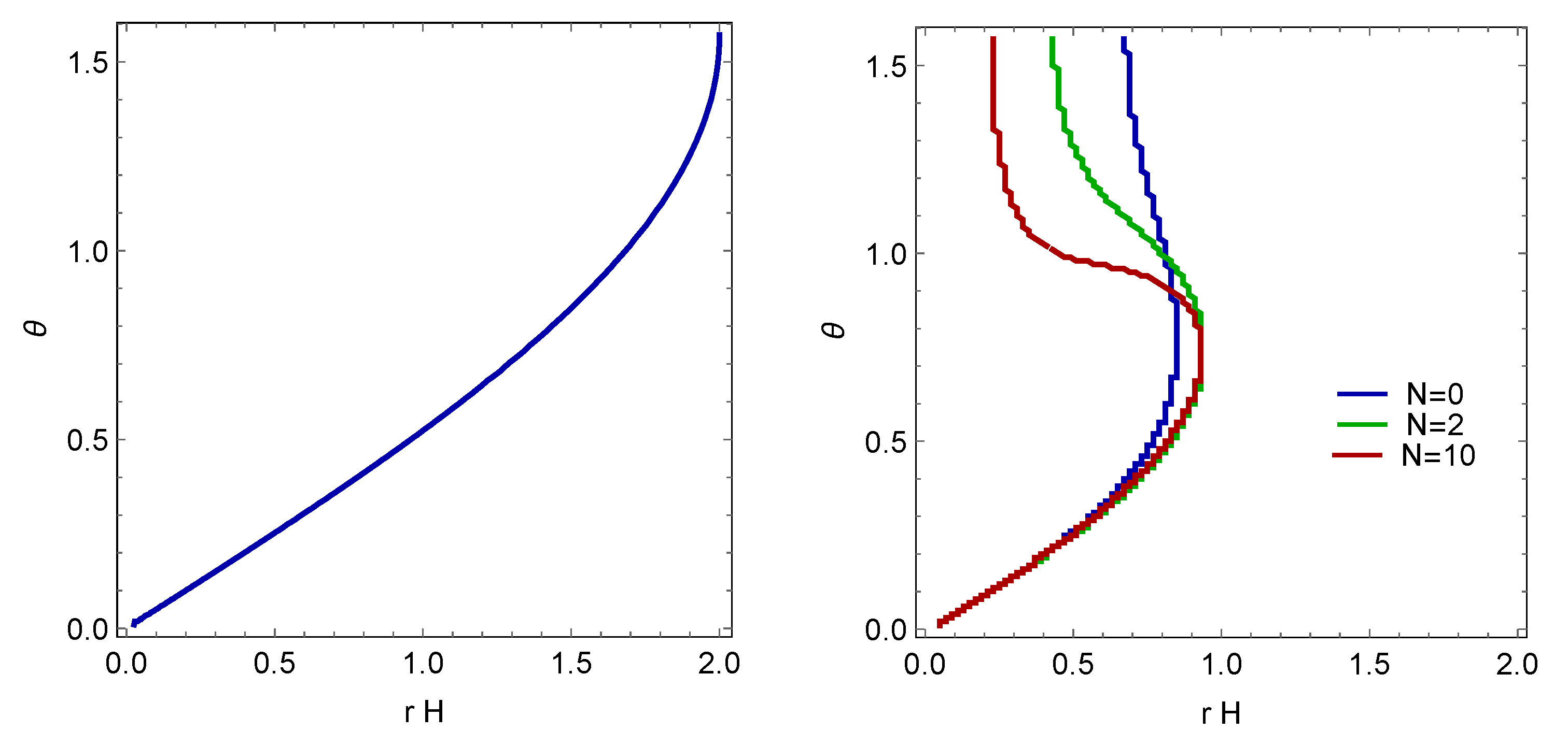
Figure 2 shows parameter regions where entanglement detection is possible. For parameters belonging to the left side regions of each lines, the negativity is positive and a pair of detectors can harvest the entanglement of the scalar field.
For the massless conformal scalar field, the maximum distance of entanglement detection is 2 H and for the massless minimal scalar field, that distance is . In this paper, we regard the Hubble length as the horizon radius and define the super horizon scale as . Following this definition of “super horizon scale”, a pair of detectors cannot access entanglement on the super horizon scale for both type of scalar fields.
4. Negativity for m + n Detectors System
Let us consider entanglement harvesting using detectors. The initial state of detectors is assumed to be
and the state after time evolution is obtained by evaluating in Equation (10):
After partial transposition of the state with respect to the group B,
where denotes a part of spanned by the basis and is a part of spanned by the basis . As these two sets of basis are orthogonal to each other, a matrix representation of with these basis has a block diagonal structure. Hence, to obtain eigenvalues of , the only thing we have to do is to consider eigenvalues of and separately.
4.1. Eigenvalues of
The eigenvalue equation is
From the configuration of detectors we are considering, we can assume the following form of the eigenvector
where are coefficients to be determined. By applying ,
and the eigenvalue equation is reduced to be
Thus,
By eliminating , we obtain
and eigenvalues are
These quantities are .
4.2. Eigenvalues of
We will show that eigenvalues of are positive up to and they do not contribute to the negativity in the present order of calculation. We assume the form of the eigenvector as
where are coefficients to be determined. By applying ,
From this, we have the following equations
After eliminating coefficients , we obtain
and eigenvalues are
Thus, up to , does not have negative eigenvalues.
4.3. Negativity
As the does not have negative eigenvalues, the negativity of the bipartite state is given by the eigenvalue of and we obtain the following key formula of the negativity in this paper
For a fixed value of the total number of detectors ,
and if the total number of detectors is even, provides a maximum value of the negativity
Figure 3 shows an example of detection of super horizon scale entanglement with ten detectors. In this case, ten detectors catch nonzero negativity on the super horizon scale r = 2.8 H.
Using Equation (14), the negativity for the massless conformal scalar field is
For a given n and separation d of detectors in the same group, we introduce a ratio with . Then, the maximum distance of entanglement detection is given by
For , we have
and can become super horizon scale as n increases. For , in the limit of large , approaches the following asymptotic value
For the massless minimal scalar field, although we cannot obtain the analytic expression of , it is possible to obtain the asymptotic formula. For with ,
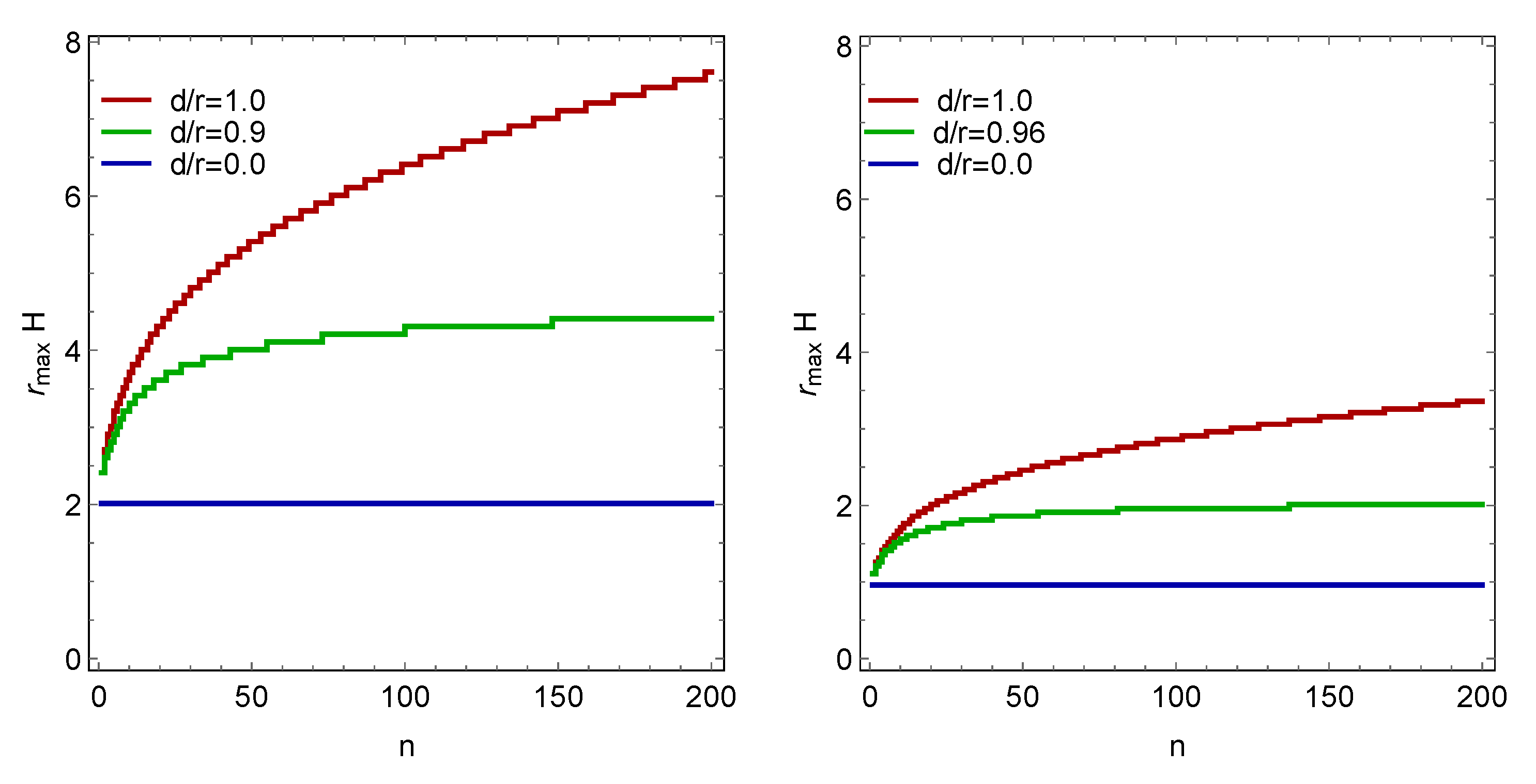
For with , can exceeds 2 H for greater than ≈0.96. Figure 4 shows as a function of number of detectors n.
For both types of scalar fields, approaches constant values as for . These constant values become larger than 2 H if is sufficiently close to unity. If we take , grows as the number of detectors increases and becomes infinity as . Therefore, it is possible to detect the super horizon scale entanglement if we prepare sufficiently large number of detectors.
5. Monogamy Inequality
We expect that detectability of large scale entanglement on the super horizon scale is related to multipartite entanglement. To make the connection clear, we check the monogamy inequality of negativity [16] for the present detectors system. For a tripartite system , the negativity between A and , between A and and between A and should obey the following monogamy inequality
This inequality implies
where and . For the present detectors model with , the left hand side of the inequality (51) is
and the right hand side of the inequality (51) is
As , which can be directly confirmed from Equations (14) and (15), the inequality (51) definitely holds.
The difference between both side of the inequality (51) can be interpreted as the residual entanglement and regarded as quantifying degrees of multipartite entanglement [16]. This quantity is
If we take , this difference becomes zero and reduces to 2 H for the massless conformal scalar case, which is the same value attained by a pair of detectors. The residual entanglement becomes maximum for , in which case can become larger than the Hubble horizon scale provided that sufficiently large number of detectors are prepared. Thus, the effect of multipartite entanglement is crucial for detection of the bipartite entanglement on the super horizon scale.
6. Summary
We investigated detection of entanglement of the scalar field on the super horizon scale in de Sitter space using multiple detectors. For this purpose, we obtained the formula of the negativity for an qubit detectors system. The maximum possible distance of detecting nonzero values of negativity is bounded by for the massless conformal scalar field and for the massless minimal scalar field. For both type of scalar fields, these bounds grow as the number of detectors increases. Thus, it is possible to detect entanglement on the super horizon scale if we prepare sufficient large number of detectors.
As a practical method to confirm entanglement of a detectors system, the test of Bell-CHSH [17] inequality for a pair of detectors is usually accepted. In our previous studies [2,4], we have confirmed that there is no violation of Bell-CHSH inequality on the super horizon scale. However, there is a possibility that effect of multipartite entanglement can violate Bell-like inequalities. Bell-Mermin-Klyshoko (BMK) inequalities [18,19,20] is such a candidate which can capture multipartite entanglement. Several authors discuss cosmological implication of this inequalities [21]. It may be interesting task to evaluate degrees of violation of these inequalities for the present detectors model.
Acknowledgments
We would like to thank S. Ishizaka for informing us monogamy relation of negativity for qubit system. This work was supported in part by the JSPS KAKENHI Grant Number 16H01094.
Author Contributions
Both authors contributed equally to this work. Both authors have read and approved the final manuscript.
Conflicts of Interest
The authors declare no conflict of interest.
References
- Steeg, G.V.; Menicucci, N.C. Entangling power of an expanding universe. Phys. Rev. D 2009, 79. [Google Scholar] [CrossRef] [Green Version]
- Nambu, Y.; Ohsumi, Y. Classical and quantum correlations of scalar field in the inflationary universe. Phys. Rev. D 2011, 84. [Google Scholar] [CrossRef]
- Martín-Martínez, E.; Menicucci, N.C. Cosmological quantum entanglement. Class. Quantum Gravity 2012, 29. [Google Scholar] [CrossRef]
- Nambu, Y. Entanglement Structure in Expanding Universes. Entropy 2013, 15, 1847–1874. [Google Scholar] [CrossRef]
- Kukita, S.; Nambu, Y. Entanglement dynamics in de Sitter spacetime. arXiv, 2017; arXiv:1706.09175. [Google Scholar]
- Nambu, Y. Entanglement of quantum fluctuations in the inflationary universe. Phys. Rev. D 2008, 78. [Google Scholar] [CrossRef]
- Nambu, Y.; Ohsumi, Y. Entanglement of a coarse grained quantum field in the expanding universe. Phys. Rev. D 2009, 80. [Google Scholar] [CrossRef]
- Matsumura, A.; Nambu, Y. Large Scale Quantum Entanglement in de Sitter Spacetime. arXiv, 2017; arXiv:1707.08414. [Google Scholar]
- Lidar, D.A.; Bihary, Z.; Whaley, K. From completely positive maps to the quantum Markovian semigroup master Equation. Chem. Phys. 2001, 268, 35–53. [Google Scholar] [CrossRef]
- Schaller, G.; Brandes, T. Preservation of positivity by dynamical coarse graining. Phys. Rev. A 2008, 78. [Google Scholar] [CrossRef]
- Benatti, F.; Floreanini, R.; Marzolino, U. Entangling two unequal atoms through a common bath. Phys. Rev. A 2010, 81. [Google Scholar] [CrossRef]
- Majenz, C.; Albash, T.; Breuer, H.-P.; Lidar, D.A. Coarse graining can beat the rotating-wave approximation in quantum Markovian master equations. Phys. Rev. A 2013, 88. [Google Scholar] [CrossRef]
- Nambu, Y.; Kukita, S. Derivation of Markovian Master Equation by Renormalization Group Method. J. Phys. Soc. Jpn. 2016, 85. [Google Scholar] [CrossRef]
- Peres, A. Separability Criterion for Density Matrices. Phys. Rev. Lett. 1996, 77, 1413–1415. [Google Scholar] [CrossRef] [PubMed]
- Horodecki, M.; Horodecki, P.; Horodecki, R. Separability of mixed states: Necessary and sufficient conditions. Phys. Lett. A 1996, 223, 1–8. [Google Scholar] [CrossRef]
- Ou, Y.-C.; Fan, H. Monogamy inequality in terms of negativity for three-qubit states. Phys. Rev. A 2007, 75. [Google Scholar] [CrossRef]
- Clauser, J.; Horne, M.; Shimony, A.; Holt, R. Proposed Experiment to Test Local Hidden-Variable Theories. Phys. Rev. Lett. 1969, 23, 880–884. [Google Scholar] [CrossRef]
- Mermin, N.D. Extreme quantum entanglement in a superposition of macroscopically distinct states. Phys. Rev. Lett. 1990, 65, 1838–1840. [Google Scholar] [CrossRef] [PubMed]
- Belinskii, A.V.; Klyshko, D.N. Interference of light and Bell’s theorem. Physics-Uspekhi 1993, 36, 653–693. [Google Scholar] [CrossRef]
- Gisin, N.; Bechmann-Pasquinucci, H. Bell inequality, Bell states and maximally entangled states for n qubits. Phys. Lett. A 1998, 246, 1–6. [Google Scholar] [CrossRef]
- Kanno, S.; Soda, J. Infinite violation of Bell inequalities in inflation. arXiv, 2017; arXiv:1705.06199. [Google Scholar]
Figure 1.
Setup of a detectors system. The group A consists of m detectors and the group B consists of n detectors. The separation between two groups is r and size of each group is d. We assume .
Figure 1.
Setup of a detectors system. The group A consists of m detectors and the group B consists of n detectors. The separation between two groups is r and size of each group is d. We assume .
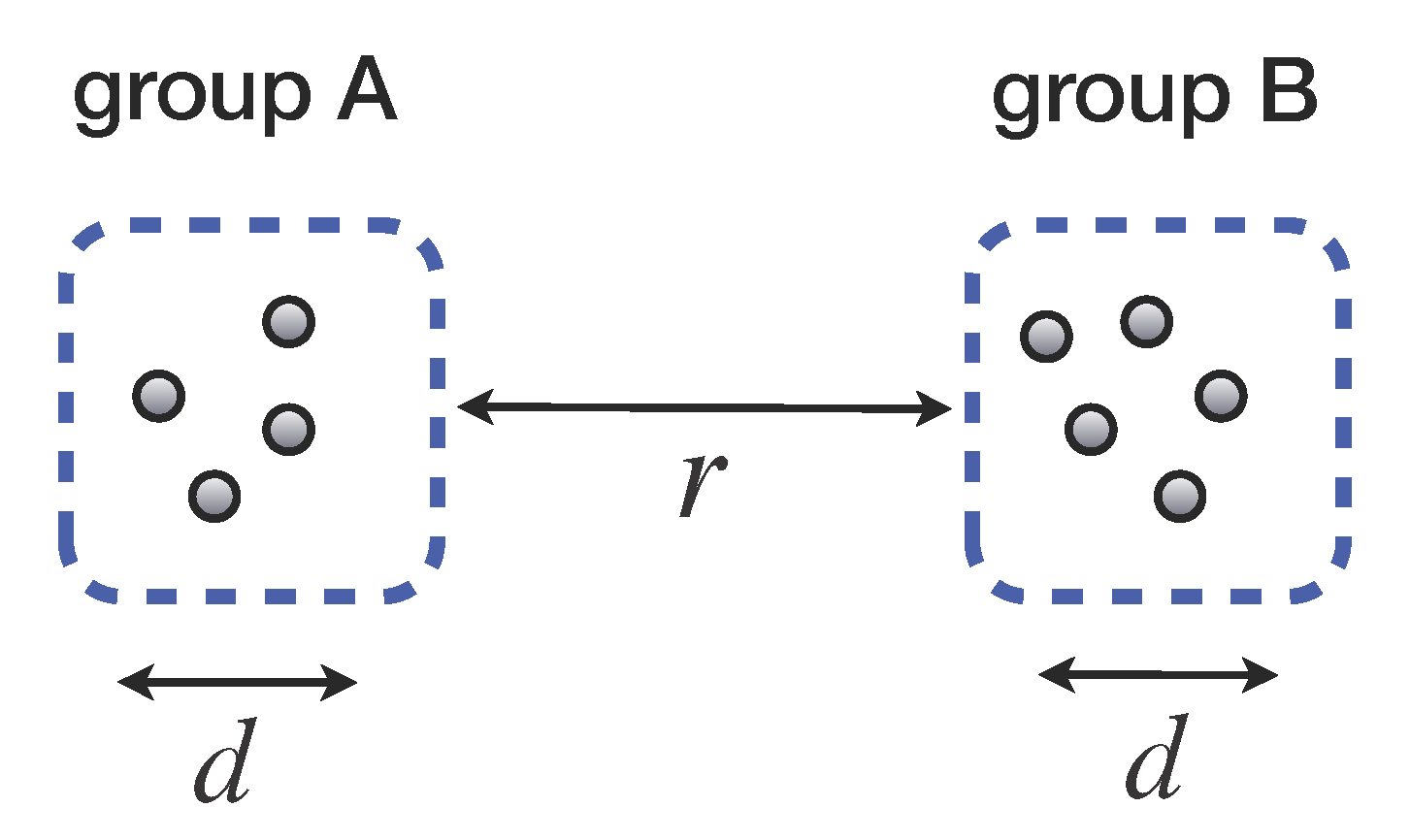
Figure 2.
The entanglement detection is possible for parameters in regions left side of each solid lines. Left panel: massless conformal scalar field. Right panel: massless minimal scalar field with e-foldings .
Figure 2.
The entanglement detection is possible for parameters in regions left side of each solid lines. Left panel: massless conformal scalar field. Right panel: massless minimal scalar field with e-foldings .

Figure 3.
Dependence of number m of group A on negativity (the massless conformal scalar field with ). The total number of detectors is with r = 2.8 H (super horizon scale). The maximum value of the negativity is attained for .
Figure 3.
Dependence of number m of group A on negativity (the massless conformal scalar field with ). The total number of detectors is with r = 2.8 H (super horizon scale). The maximum value of the negativity is attained for .
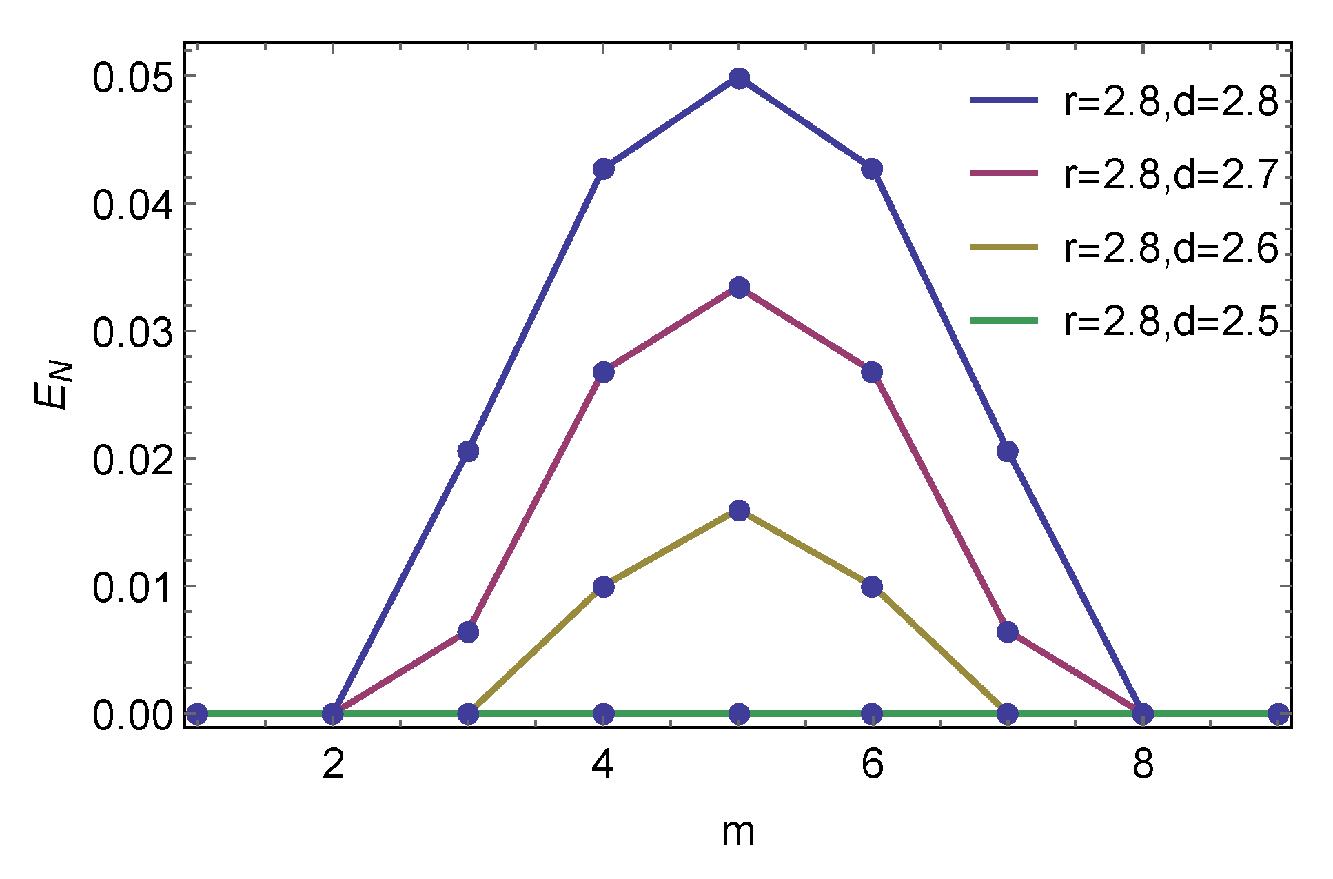
Figure 4.
as a function of number of detectors n. Left panel: the massless conformal scalar field with . Right panel: the massless minimal scalar field with . For both types of scalar fields, with , exceeds the horizon scale 2 H as the number of detectors increases.
Figure 4.
as a function of number of detectors n. Left panel: the massless conformal scalar field with . Right panel: the massless minimal scalar field with . For both types of scalar fields, with , exceeds the horizon scale 2 H as the number of detectors increases.
© 2017 by the authors. Licensee MDPI, Basel, Switzerland. This article is an open access article distributed under the terms and conditions of the Creative Commons Attribution (CC BY) license (http://creativecommons.org/licenses/by/4.0/).
Share and Cite
MDPI and ACS Style
Kukita, S.; Nambu, Y. Harvesting Large Scale Entanglement in de Sitter Space with Multiple Detectors. Entropy 2017, 19, 449. https://doi.org/10.3390/e19090449
AMA Style
Kukita S, Nambu Y. Harvesting Large Scale Entanglement in de Sitter Space with Multiple Detectors. Entropy. 2017; 19(9):449. https://doi.org/10.3390/e19090449
Chicago/Turabian StyleKukita, Shingo, and Yasusada Nambu. 2017. "Harvesting Large Scale Entanglement in de Sitter Space with Multiple Detectors" Entropy 19, no. 9: 449. https://doi.org/10.3390/e19090449
Note that from the first issue of 2016, this journal uses article numbers instead of page numbers. See further details here.