The Thermodynamical Arrow and the Historical Arrow; Are They Equivalent?

Department of Mathematics, University of Stockholm, 106 91 Stockholm, Sweden
Entropy 2017, 19(9), 455; https://doi.org/10.3390/e19090455
Submission received: 29 June 2017
/
Revised: 26 August 2017
/
Accepted: 28 August 2017
/
Published: 30 August 2017
(This article belongs to the Special Issue Entropy, Time and Evolution)
Abstract
:In this paper, the relationship between the thermodynamic and historical arrows of time is studied. In the context of a simple combinatorial model, their definitions are made more precise and in particular strong versions (which are not compatible with time symmetric microscopic laws) and weak versions (which can be compatible with time symmetric microscopic laws) are given. This is part of a larger project that aims to explain the arrows as consequences of a common time symmetric principle in the set of all possible universes. However, even if we accept that both arrows may have the same origin, this does not imply that they are equivalent, and it is argued that there can be situations where one arrow may be well-defined but the other is not.
1. Introduction
This paper is a part of a project that is aimed at an explanation of the asymmetry of time as a broken symmetry in the set of all possible universes; it can be that a definite direction of macroscopic time is simply, by far the most common situation, even if we consider both the underlying microscopic laws and the boundary conditions to be symmetric.
However, in the discussions related to this project, it has turned out that there is still a lot of confusion about the meaning of time asymmetry, and in particular as to whether different criteria for time asymmetry are equivalent or not.
This may not be strange in view of the fact that questions about time often involve statements about our universe that may be enormously complex. Nevertheless, it is a problem for the discussion.
In the following I will focus on the relation between two of the most important manifestations of time asymmetry: the thermodynamic and the historical arrows, rather than discussing the origin of time asymmetry in general. Hence, I have for most of this paper chosen to work within a framework that makes sense also for open universes, where the asymmetry is, so to speak, built in from the beginning. Still, to make the relationship to the general project clearer, a short description of the situation for closed universes, where the breaking of time symmetry is the main point, is given in Section 10.
There have been many attempts to investigate time asymmetry in the context of specific theories (see e.g., [1,2,3,4,5,6,7,8,9]). Here the method of attack is in a sense the opposite one—to create an extremely simple framework, where the different arrows of time can be viewed as consequences of very fundamental statistical principles, rather than as, e.g., quantum phenomena.
In this paper, each possible universe is considered as a path in the graph of all possible states. This model is clearly a very crude one, but it is my hope that it is in fact an abstraction on the right level for an understanding of at least some of the main aspects of the asymmetry of time.
2. Historical Background
Time’s Arrow is the name coined by Eddington [10] to indicate the direction from the past towards the future. However, how do we know in what direction it points? Or in other words, what is it that makes the future different from the past? There are several different answers, or “Arrows”, i.e., ways to distinguish the past and future, that have been proposed. According to the article by Hartle and Gellmann in [8] (see also Zeh [9]), there are at least six or seven different arrows.
The most common ones are perhaps
The Thermodynamic Arrow:
The future is the direction of time in which entropy increases.
The arrow defined by the increase of entropy essentially goes back to Boltzmann [11] (although the name came later).
The Psychological Arrow:
The past is the direction of time in which we can remember, as opposed to the future which we can not remember.
Since the psychological arrow is based on human intuition and our ability to remember, it is in essence probably as old as our ability to think about time at all. However, at the same time, involving human psychology obviously leads to problems in a scientific discussion. A slight modification of the psychological arrow is
The Historical Arrow:
The past is the direction of time in which there is a history.
Here all direct references to human psychology are gone, since we can in principle imagine history without any experiencing subject. Still, it is unclear exactly what “history” should mean. I will come back to this question in Section 3.
Another example is the Cosmological Arrow, which points in the direction in which the universe expands. It has the property that it is well-defined even in the very early history of the universe, where it is not obvious that the other arrows make sense. There is a long going discussion about the relation between the cosmological arrow and the thermodynamic arrow (see [12,13,14]. For a somewhat more recent account, see [7]).
All of the above arrows are, to their nature, macroscopic concepts. When we study microscopic situations, they loose their meaning. A possible exception to this could be “the Decoherence Arrow”, which, in a sense, can be observed on the microscopic level [9]. There does not appear to be any consensus in the scientific community as to whether this truly is a microscopic arrow, or if it just reflects our well-known ability to choose very exceptional initial states for our experiments.
It is an important dividing line between different kinds of explanations of the asymmetry, whether or not we assume that, on the microscopic level, the laws of physics are essentially time-symmetric (time development is unitary). If (essentially) every development on the micro level, which is possible in one direction of time, is also possible in the other, then we can not really use microscopic laws to distinguish between the future and the past. Time symmetry on the micro level is essential for the approach that this paper is a part of. For an interesting discussion of the opposite approach, where rather non-unitarity itself is taken as the starting point, see [15] (and further references given there).
Are the different arrows equivalent? In other words, will they always point in the same direction in any physical situation? If so, why? If not, under what circumstances may they fail to coincide? These are very complicated questions, and I will in the following restrict myself to a few aspects, mainly concerning the thermodynamic and the historical arrows.
3. Conceptual Problems
The thermodynamic arrow is very intimately connected with the second law of thermodynamics. This second law, it was once argued by Eddington ([10], p. 74), is the most unquestionable law of physics that we have. In view of more recent research, this statement may have been somewhat over exaggerated (see e.g., [16]). Nevertheless, under most ordinary circumstances, we have a good understanding of how entropy should be computed, at least in principle.
However, the situation becomes more complicated if we turn to cosmology and try to consider the entropy of the whole universe. In particular, different generalizations of the usual concept of entropy can give different results, depending on whether we use classical physics or quantum physics and on how the expansion of the universe is taken into account. In fact, without pushing the analogy too far, the situation is to a certain extent similar to the problems with the first law of thermodynamics, where (gravitational) energy under normal circumstances is a well understood concept, but where it becomes problematic to define it for the universe as a whole.
There is also a problem with the concept of time itself, as was already noted by Augustinus (“What, then, is time? If no one ask of me, I know; if I wish to explain to him who asks, I know not.” (From Confessiones)). As long as we do not fully understand what time is, it is easy to commit errors when discussing time’s arrow. For a discussion of these matters, see [17].
As already mentioned in Section 2, the meaning of the historical arrow is not at all clear from the beginning, and hence it must be made more precise before we can go further. A possible starting point is that in quantum physics, there are many phenomena that are genuinely unpredictable, e.g., the future decay of a neutron. Although the probability for such a decay can be well predicted by quantum mechanics, the consequences of the decay tend to be chaotic and may hence lead to completely different futures within a comparatively short time. On the other hand, the past always seems to be well-defined, at least if we avoid questions on the micro level like “which slit did the photon pass through?”.
Hence, a possible way of making the historical arrow more precise would be:
The Historical Arrow:
The past is the direction of time in which the development that we observe is uniquely determined, whereas the future is the direction in which the development is not uniquely determined.
Several alternative names for this arrow would be possible, each with its own merits and drawbacks. One possible choice would be the “The Determinedness Arrow”. In fact, the “historical arrow” has already been used with a slightly different meaning (see e.g., [18]).
The historical arrow is also very closely connected with the multiple history view of the world, where different possible futures are considered to be equally real. As will be further discussed below, the historical arrow can be viewed as a kind of combinatorial property of the multiverse.
Finally, there is a problem with the concept of “states”. To say that the future is not unique means that the state we experience right now can give rise to different states in the future. However, exactly what is a “state”? Quantum mechanics is a completely deterministic theory in the sense that the Schrödinger equation for the wave function can be solved uniquely both backwards and forwards in time. In particular, time development gives an isomorphism between the quantum states at any two different moments of time.
However, the problem is that, if interpreted in the usual quantum mechanical way, the different futures that may result from what we experience now are all governed by the same wave function, which we can never fully describe. Therefore, the macroscopic “states” that we observe are quite different from ordinary quantum mechanical states. In particular, time development does not give an isomorphism between these states at two different moments of time, and it is quite possible to imagine all possible developments as starting from just one single state at the Big Bang.
To try to solve all these conceptual problems at the same time would, in my opinion, simply be to ask too much. In this paper, I will instead choose a different path. By considering a very simplified model for the multiverse, most of the above problems can be avoided, and the different arrows can then be investigated by very simple mathematical methods. It is, of course, not evident that such a model will give the right solution to the riddle of time’s arrow. However, it does give a conceptual framework where the arrows can be well understood.
4. The Combinatorial Multiverse
Presently, the two most common interpretations of quantum mechanics are the Copenhagen interpretation and the multiverse interpretation. Both of them have been promoted and criticized for various reasons, a discussion that I do not want to enter here.
Still, the underlying perspective in this paper is essentially the “democracy of all histories” perspective, even if it may differ somewhat from the usual Everett interpretation [19]. All possible developments starting from the Big Bang are considered on equal terms. The point is that the set of all such developments form a completely deterministic mathematical structure with its own deterministic laws. Thus, we can create models for this set (“the multiverse”), which can be studied in their own right. And it may then be the free metaphysical choice of the reader whether or not to give our own present development a special ontological status (at the price of introducing a stochastic point of view).
In the following, each possible universe will be viewed as a path in a huge graph. Time will be assumed to be discrete and, choosing appropriate units and simplifying somewhat, we may take the moments of time to be the (positive) integers.
For each moment t during the life span I of the multiverse, we let denote the set of all possible states, and the totality of all states will then be denoted by
ℵ can be thought of as a kind of “super-space” in the original sense of Wheeler [20]. In the following, the sets will always be finite for a given t. This is not a necessary assumption, but for obvious reasons it simplifies the probabilistic treatment. As for the interval I, it may be finite or infinite, corresponding to closed and open universes. In view of the enormous complexity of this ℵ, it is necessary to make drastic simplifications, and the main idea of the model in this paper is to suppress all dynamical properties except for entropy.
According to Boltzmann, the total entropy of a certain macro-state at a certain time is given by
or inversely
where denotes the number of corresponding micro-states, and is Boltzmann’s constant. Although this formula was derived under quite special circumstances, it is generally agreed to contain an almost universal truth about nature. In particular, I will, in the following, take for granted that the total number of possible (micro-)states of a universe, with a given entropy S at a particular moment of time, is an exponential function of the total entropy as in (3).
In the discussion below, macro-states will play no role at all. Therefore, I will drop the prefix micro- and just write “state” instead of “micro-state” from now on.
Remark 1.
If the total number of states is finite, then the assumption, about the exponential dependence of the number of states as a function of entropy, can of course only hold true as long as the entropy is not near to becoming maximal. However, we are not there yet, and according to [21,22], it would take a very long time indeed for our universe to reach such a state.
It is not a all evident that W should be considered to be independent of t. In fact, this is a situation where it does matter how we generalize the concept of entropy to the universe as a whole; according to (3), the dependence of W on t is directly related to how we measure entropy. In particular, it should be made clear how the expansion of the universe in itself contributes to the growth of entropy. Fortunately for this paper, such a dependence of W on t would only have a minor influence on the ideas in the following, therefore I will, for simplicity, assume W to be constant. It is however possible that a more complicated behavior of W, e.g., near the Big Bang or a possible Big Crunch, could have interesting consequences.
As for the starting point itself at time (the Big Bang), I will simply assume that consists of just one state with zero entropy, i.e., that every universe starts from a completely ordered state (of zero volume). (If we consider a closed multiverse, there should of course be a similar condition at the right end).
It is also necessary to specify the dynamics of the model. For a given state at a given moment of time t, the dynamical laws will only permit transitions to a very limited number of states at the next moment of time. Needless to say, in reality, the laws of quantum mechanics make no absolute distinction between possible and impossible transitions, but for the purpose of this paper, I will still make this simplifying assumption.
In the combinatorial model under study here, this corresponds to specifying the edges between states at adjacent moments of time; the presence of an edge between the states indicates that the transition is possible, and the absence of such an edge indicates that the corresponding transition is not possible. In this way, ℵ now becomes a graph.
Putting everything together, we arrive at:
Definition 1.
A universe is a path in the graph ℵ, i.e., a chain of states (one state for each moment of time t), with the property that the transition between adjacent states is always possible.
Definition 2.
The multiverse M is the set of all possible universes Ξ in the sense of Definition 1.
5. The Strong Arrows of Time in the Combinatorial Multiverse
In the simple context of the previous section, we can now interpret different arrows as different dynamical properties of the multiverse.
The Strong Thermodynamic Arrow:
A model for the multiverse is said to possess a strong (forward) thermodynamic arrow on the interval if whenever an edge connects a state at time t to a state at time , where , the entropy of is strictly larger than the entropy of .
The Strong Historical Arrow:
A model for the multiverse is said to possess a strong (forward) historical arrow on the interval if for every state at time , there is at most one edge leading to a state at time , but strictly more than one edge leading to states at time .
Note that in a closed model for the multiverse, including a Big Crunch, there are obvious analogous definitions of backwards arrows.
Let us also note that the strong arrows are not compatible with completely time-symmetric laws on the micro level. In fact, no development would be time reversible in the presence of the strong arrows. Consequently, if we want to argue in favor of a strong arrow it also means that we consider time asymmetry to be built into the dynamics itself.
6. The Weak Arrows of Time in the Combinatorial Multiverse
One obvious conclusion from the previous section is that if we do believe that the dynamics are essentially time symmetric, then we must look for other weaker ways to define the arrows.
A possible way to proceed is to consider the multiverse as a probability space and argue that universes that possess arrows are far more likely than those without. In this section, the probability measure on ℵ will be the simplest possible one: each universe is given the same probability weight.
The Weak Thermodynamic Arrow:
A model for the multiverse is said to possess a weak (forward) thermodynamic arrow on the interval , if the total probability of all universes with monotonically increasing entropy is very close to one.
The Weak Historical Arrow:
A model for the multiverse is said to possess a weak (forward) historical arrow on the interval , if the total probability of all universes where at each moment of time, the history is unique but the future is not unique, is very close to one.
In other words, no other universe will pass through any of the states for , but for any , , there will be at least one more universe that agrees with the given one up to , but differs from it at time .
Again, in a closed model for the multiverse, there are obvious analogous definitions of backwards arrows.
In order to make the above definitions precise, we have to give an exact meaning to the expression “very close to”. The most rigorous way would be to deal with the limit case where the interval of time, the number of states, etc. tend to infinity, in very much the same way as, e.g., phase transitions in statistical mechanics can be defined in terms of “thermodynamic limits” (see, e.g., Ruelle [23]).
However, in order not to make the discussion more technical than necessary, I will, in the next section, only discuss an explicit simple model for the dynamics of the multiverse. The main point is that, as opposed to the case with the strong arrows in Section 5, this kind of essentially time-symmetric dynamics may, in a certain sense, be compatible with the weak arrows as defined above, see the discussion in Section 8.
7. Symmetric Boltzmann Dynamics
The Symmetric Dynamic Principle (SDP):
For any state at time t with entropy S (with obvious modifications at the end point(s)), there are exactly K edges connecting to different states at time with entropy , and these will be chosen completely at random among such states. Similarly, there will be exactly the same number K of edges connecting to different states at time with entropy .
Note that all edges in the model are defined in this way: in particular, passage from one state to another along such an edge will always change the entropy by .
This Principle is very closely related to Boltzmann’s ingenious idea that the second law of thermodynamics is a manifestation of the fact that our universe develops from less probable to more probable states. However, the point is: now the formulation is time symmetric.
Remark 2.
If the multiverse itself is a completely deterministic structure, why should we appeal to randomness in the SDP above? The answer is that randomness is just a way to simulate a much more complex dynamical behavior and at the same time it makes computing much easier. In a more realistic approach based on, say, the Schrödinger equation, no such random choice would be necessary, but on the other hand the computational difficulties would rapidly become enormous.
Clearly, the assumption that the edges from a given state are chosen completely at random is a very coarse one, which can not possibly give an accurate explanation of any kind of detailed behavior of the multiverse.
In the following, it is important that W in (3) is much larger than the K in the SDP. In other words,
will always be a very small number.
Observation 1.
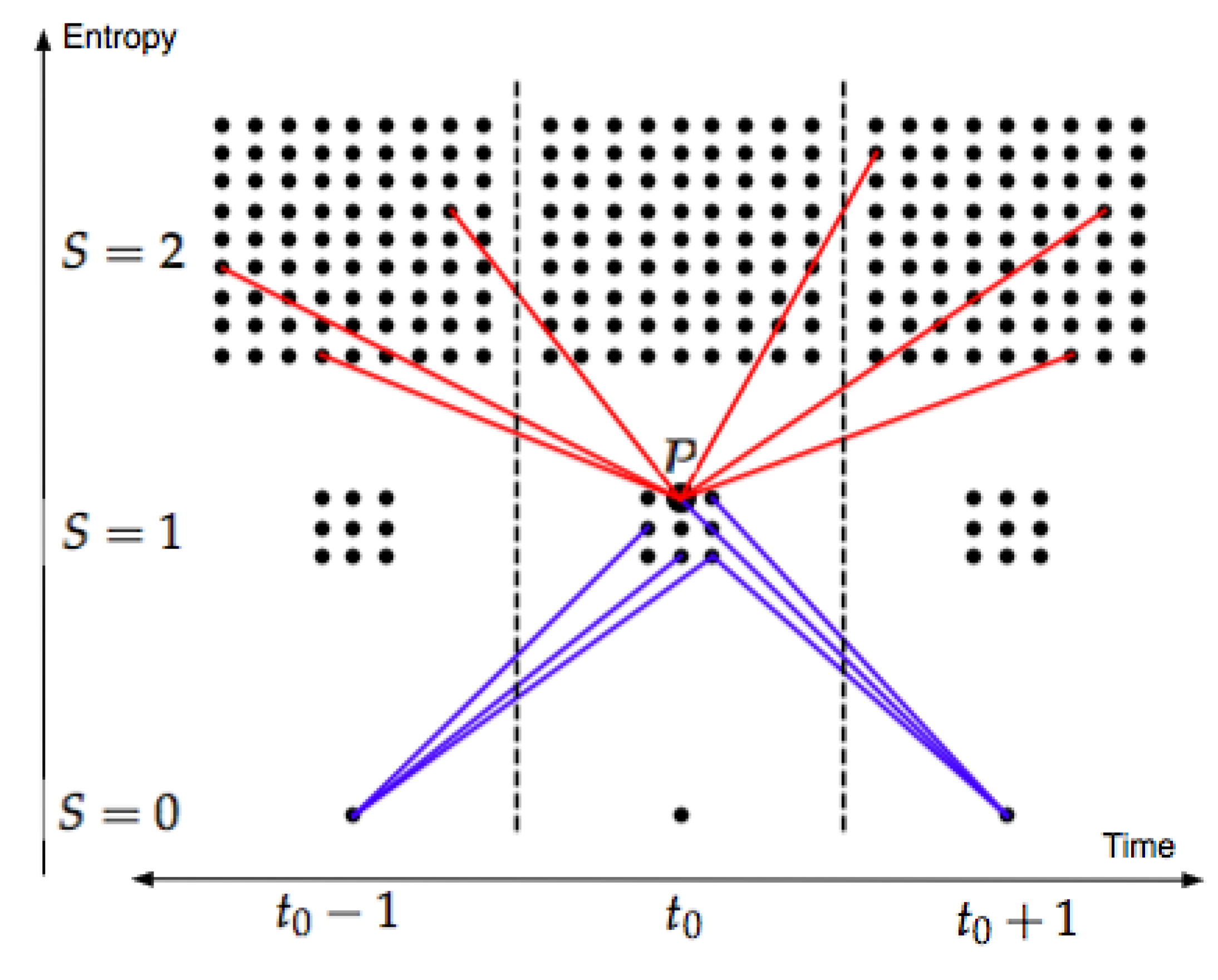
In particular, this means that among all states with entropy S at a certain moment of time t, only a minor fraction can be reached from states with lower entropy at times or . In other words, only comparatively few states have edges connecting to states with lower entropy in any of the two directions of time. Actually, the small number δ can be interpreted as an upper bound for the probability of randomly chosen states with entropy S at time t to have an edge connecting it to a state at time (or ) with entropy . In fact, starting from the states at time , we know from (3) that there are of them, and according to the SDP each of these can connect to K states with entropy S at time t. We conclude that at most states among the states with entropy S at time t can connect to the given states at time with entropy , which gives the probability
(note the “at most”, since some of the edges may connect to the same state at time t). An example of this situation, with very small values of W, K and S, is given in Figure 1.
8. The Weak Arrows in the Combinatorial Multiverse
Using statistical reasoning, it is now not difficult to estimate the number of universes with monotonic/non-monotonic behavior of the entropy.
Starting from the unique state with entropy at the Big Bang, there are, after one unit of time, K accessible states with . After two units of time there are different paths leading to states with , and so on. Hence, after N units of time, there are different paths (universes) with , and these are clearly exactly the ones with monotonically increasing entropy.
On the other hand, the number of universes with non-monotonic entropy can be estimated as follows. If the entropy is non-monotonic, then at k moments of time the entropy must instead decrease by one, where . This gives the following upper bound for the total number of such states (note that we get a strict inequality, since the requirement that restricts the number of possible combinations. For instance, is a necessary condition.)
The ratio between the number of non-monotonic and monotonic universes p therefore satisfies
(note that the ≈ in (6) is justified in this case). Hence, we arrive at the following
Claim 1.
In the limit , the model exhibits a weak thermodynamic arrow.
If we instead turn to the historical arrow, then a corresponding argument may look as follows:
Arguing as above, we see that the number of possible universes up to time N is . The probability that a given universe does not have a unique history up to time N can be estimated by
where is the probability that after k units of time there is another path from the Big Bang to the corresponding state of . This probability can clearly, using our statistical assumption, be estimated by , since is the number of possible universes and is (approximately) the number of possible states at time k. Hence, we arrive at the expression
which, since , can be approximated by just the first term . Therefore, the probability q that a given universe has a non-unique history after N units of time satisfies
which implies
Claim 2.
In the limit , the model exhibits a weak historical arrow.
9. Discussion
In Section 8, I have discussed different criteria for the existence of weak thermodynamic and historical arrows in the combinatorial model, as expressed by Claims 1 and 2.
In particular, we see that the Symmetric Dynamic Principle implies the existence of both arrows if .
The condition is an extremely natural one if we attempt to model a world similar to the one we know—without any condition of this kind, too many developments would be possible and the world would be quite chaotic.
Remark 3.
The condition is somewhat different. If N is too large, then, of course, sooner or later a violation of monotonicity will occur, simply because if we repeat any experiment sufficiently many times, even the most unlikely outcome will eventually occur. This does not necessarily imply anything essential about the second law.
In fact, in a more realistic model it may also be that the historical arrow will be violated if N is very large. The reason is that in the real world, the dynamics implied by the SDP are too simple—the chance that two universes will meet at a certain time is of course not independent of their previous histories. Rather, universes that separated not long ago will have greater chances to reunite. In fact, this may, in a sense, be essentially what happens in quantum physics where different developments do interact.
Nevertheless, it is the opinion of the author that these effects are secondary, and if we accept that our history is not nearly long enough for N to become comparable to W, then, to a first approximation, the Claims 1 and 2 really, in a certain sense, do offer an explanation to the question why we live in a world with both a thermodynamic and a historical arrow.
However, the fact that both arrows may be viewed as consequences of one and the same dynamic principle (in this case the Symmetric Dynamic Principle) does not necessarily imply that they are equivalent. So we must also ask ourselves if there can be situations where one of the arrows may fail to exist but the other is still well-defined?
The thermodynamic arrow may fail to exist if the system reaches a state of complete disorder, i.e., of maximal entropy. However, this does not imply that the historical arrow will disappear. In fact, if K is not too large, then even after maximal entropy has been reached there will be comparatively few possible universes, and the chance that two of them will ever meet at a single state may still be extremely small for the same reasons as in Claim 2.
In the other direction, as long as the condition is fulfilled, it does not seem to be possible to construct a model, based on the Symmetric Dynamic Principle, where the thermodynamic arrow is well-defined but the historical arrow has failed to exist. So in a certain sense, in the context of the present combinatorial model, it appears that the historical arrow may in a sense be more general than the thermodynamic arrow.
However, close to the Big Bang (and a possible Big Crunch), the situation may be quite different. In a situation where quantum effects may dominate the whole multiverse, it is not at all clear that the Symmetric Dynamic Principle or the thermodynamic and historical arrows will have any sensible interpretation at all. If they still have, it is not even clear that they could not point in different directions. In fact, even the strong arrows of Section 5 could in principle point in different directions if the dynamics are very special, although their definitions put very severe conditions on the length of a time interval with this property.
Thus, it is the opinion of the author that we must be very careful when presupposing any kind of arrow of time (except for the cosmological one) under such circumstances. This has little impact on the discussion of the open multiverse, which is the main theme in this paper, since it can be taken for granted that all universes will come out of these very first moments of time in states of very low entropy. However, the situation is quite different in the case of a closed multiverse, as will be discussed in the next section.
10. The Origin of Time’s Arrow in the Multiverse
In this section, I will make a digression from the main line of this paper to briefly describe how the SDP is related to the problem of time asymmetry in general. General references for this discussion are [24,25,26].
In the discussion of the two arrows in Section 9, we specifically studied universes starting from a low entropy Big Bang, thus in a sense already presuming a definite direction of time. On the other hand, the future of the multiverse was, so to speak, left open.
However, what happens in a closed multiverse with finite volume and with a Big Bang in one end and a Big Crunch in the other? In the combinatorial framework of this paper, this means that every path (universe) must start and end at unique states with entropy zero. This is clearly not compatible with any of the arrows discussed in Section 5 and Section 6.
Can some conclusions still be drawn from the SDP? The point here is that, as was mentioned in Section 9, the physics of the very first (and last) moments of a real multiverse is very extreme, and we should be very careful about assuming anything at all about arrows, entropy, etc. In fact, when the size of space is extremely small and quantum phenomena dominate, then, in a sense, any kind of development is possible, although perhaps not all with the same probability.
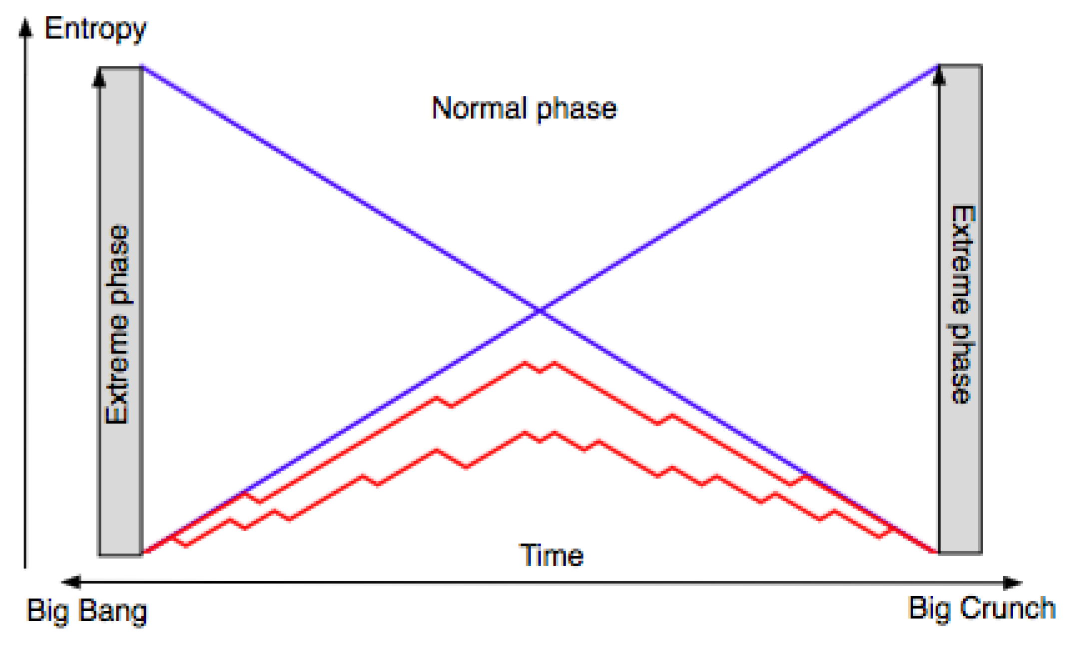
When modeling such a multiverse combinatorically, it is reasonable to assume the SDP only during the “normal phase” in between, and to model the behavior near the end points in a very different, although of course still time symmetric, way. Without entering into the details about how this can be done (see [24,25,26]), let me note that with certain assumptions, it can be argued that a monotonic behavior of the entropy during the normal phase is far more likely than a behavior with low entropy at both ends. Since we obviously live in a universe with low entropy at one end, this offers an explanation of why the entropy should be high when we approach the other end. In other words, we should observe a thermodynamic arrow during the normal phase.
It is important to note, however, that the multiverse itself is still time symmetric. Even if all observers, who are after all confined to particular universes, observe thermodynamic arrows, there will be equally many universes where the corresponding arrows point in each of the two directions. In other words, in (almost) 50% of all universes, the arrow points in the same direction as in ours. However, it is equally true that in (almost) all of the other 50%, it points in the other direction. See Figure 2.
11. Final Remark
In this paper, I have argued that in the setting of a simplified combinatorial multiverse, both the thermodynamic and the historical arrows can be viewed as consequences of essentially time symmetric dynamics, even if there may be situations where they behave differently.
However, it is also worth noting that there is another kind of difference between the two arrows. The thermodynamic arrow is an essentially classical phenomenon—if we just assume that a universe starts from a more or less randomly chosen low entropy state during the very first moments after the Big Bang, the following development towards higher and higher entropy was, in principle, already well understood by Boltzmann.
However, the historical arrow is of a different kind, in the sense that here quantum mechanics is essential. If we, e.g., study classical deterministic Newtonian mechanics, the definitions of the historical arrows make no sense at all. In the context of this paper, the condition is essential for the historical arrow even to have a meaning.
One should be careful about drawing too far reaching conclusions about this difference, in particular for the realistic dynamics of our own world. Nevertheless, it is an interesting property of the combinatorial model in this paper.
Conflicts of Interest
The author declares no conflict of interest.
References
- Bohm, A.; Antoniou, I.; Kielanowski, P. A quantum mechanical arrow of time and the semigroup time evolution of Gamow vectors. J. Math. Phys. 1995, 36, 2593–2604. [Google Scholar] [CrossRef]
- Bohm, A.; Scurek, R. The phenomenological preparation-registration arrow of time and its semigroup representation in the RHS quantum theory. In Trends in Quantum Mechanics; Doebner, H.D., Ali, S.T., Keyl, M., Werner, R.F., Eds.; World Scientific: Singapore, 2000. [Google Scholar]
- Prigogine, I.; George, C. The second law as a selection principle: the microscopic theory of dissipative processes in quantum systems. Proc. Natl. Acad. Sci. USA 1983, 80, 4590–4594. [Google Scholar] [CrossRef] [PubMed]
- Antoniou, I.; Prigogine, I. Intrinsic irreversibility and integrability of dynamics. Physics A 1993, 192, 443–455. [Google Scholar] [CrossRef]
- Earman, J. An attempt to add a little direction to The problem of the direction of time? Philos. Sci. 1974, 41, 15–47. [Google Scholar] [CrossRef]
- Castagnino, M.; Lombardi, O.; Lara, L. The global arrow of time as a geometrical property of the universe. Found. Phys. 2003, 33, 877–912. [Google Scholar] [CrossRef]
- Castagnino, M.; Lara, L.; Lombardi, O. The cosmological origin of time-asymmetry. Class. Quantum Grav. 2003, 20, 369–391. [Google Scholar] [CrossRef]
- Halliwell, J.J.; Perez-Mercander, J.; Zurek, W.H. Physical Origins of Time Asymmetry; Cambridge University Press: Cambridge, UK, 1994. [Google Scholar]
- Zeh, H.D. The Physical Basis of The Direction of Time, 4th ed.; Springer: Berlin/Heidelberg, Germany, 2001. [Google Scholar]
- Eddington, A.S. The Nature of the Physical World; Cambridge University Press: Cambridge, UK, 1928. [Google Scholar]
- Boltzmann, L. Theoretical Physics and Philosophical Problems; McGuinness, B., Ed.; Reidel Publishing Co.: Dordrecht, The Netherlands, 1974. [Google Scholar]
- Gold, T. The Arrow of Time. Am. J. Phys. 1962, 30. [Google Scholar] [CrossRef]
- Hawking, S.W. Arrow of Time in Cosmology. Phys. Rev. D 1985, 33, 1–41. [Google Scholar] [CrossRef]
- Page, D. Will the entropy decrease if the Universe recollapse? Phys. Rev. 1985, 16. [Google Scholar] [CrossRef]
- Kastner, R.E. On Quantum Collapse as a Basis for the Second Law of Thermodynamics. Entropy 2017, 19. [Google Scholar] [CrossRef]
- Čápek, V.; Sheehan, D.P. Challenges to the Second Law of Thermodynamics; Springer: Dordrecht, The Nertherlands, 2005. [Google Scholar]
- Martyushev, L.M. On Interrelation of Time and Entropy. Entropy 2017, 19. [Google Scholar] [CrossRef]
- Layzer, D. The Arrow of Time. Sci. Am. 1975, 233, 56–69. [Google Scholar] [CrossRef]
- Everett, H. Relative State Formulation of Quantum Mechanics. Rev. Mod. Phys. 1957, 29. [Google Scholar] [CrossRef]
- Misner, C.M.; Thorne, K.S.; Wheeler, J.A. Gravitation; W.H. Freeman and Company: San Fransisco, CA, USA, 1973. [Google Scholar]
- Adams, F.; Laughlin, G. A dying universe: The long-term fate and evolution of astrophysical objects. Rev. Mod. Phys. 1997, 69. [Google Scholar] [CrossRef]
- Egan, C.; Lineweaver, C. A Larger Estimate of the Entropy of the Universe. Astrophys. J. 2010, 710. [Google Scholar] [CrossRef]
- Ruelle, D. Thermodynamic Formalism; Cambridge University Press: Cambridge, UK, 1984. [Google Scholar]
- Tamm, M. Time’s Arrow from the Multiverse Point of View. Phys. Essays 2013, 26, 237–246. [Google Scholar] [CrossRef]
- Tamm, M. Time’s Arrow in a Finite Universe. Int. J. Astron. Astrophys. 2015, 5, 70–78. [Google Scholar] [CrossRef]
- Tamm, M. A Combinatorial Approach to Time Asymmetry. Symmetry 2016, 8. [Google Scholar] [CrossRef]
Figure 1.
This picture illustrates Observation 1 with and . The state P at time with entropy connects to 3 states with at time and equally many at time . However, there is no edge connecting to the (in this case) unique state with at time and only one edge connecting to the unique state with at time .

Figure 2.
A schematic picture of the entropy as a function of time for four different universes in a small combinatorial multiverse. The blue graphs represent the highly probable asymmetric cases, whereas the red ones represent highly improbable cases with low entropy at both ends.
Figure 2.
A schematic picture of the entropy as a function of time for four different universes in a small combinatorial multiverse. The blue graphs represent the highly probable asymmetric cases, whereas the red ones represent highly improbable cases with low entropy at both ends.

© 2017 by the author. Licensee MDPI, Basel, Switzerland. This article is an open access article distributed under the terms and conditions of the Creative Commons Attribution (CC BY) license (http://creativecommons.org/licenses/by/4.0/).
Share and Cite
MDPI and ACS Style
Tamm, M. The Thermodynamical Arrow and the Historical Arrow; Are They Equivalent? Entropy 2017, 19, 455. https://doi.org/10.3390/e19090455
AMA Style
Tamm M. The Thermodynamical Arrow and the Historical Arrow; Are They Equivalent? Entropy. 2017; 19(9):455. https://doi.org/10.3390/e19090455
Chicago/Turabian StyleTamm, Martin. 2017. "The Thermodynamical Arrow and the Historical Arrow; Are They Equivalent?" Entropy 19, no. 9: 455. https://doi.org/10.3390/e19090455
Note that from the first issue of 2016, this journal uses article numbers instead of page numbers. See further details here.