Economics and Finance: q-Statistical Stylized Features Galore

1
Centro Brasileiro de Pesquisas Físicas and National Institute of Science and Technology for Complex Systems, Rua Xavier Sigaud 150, Urca, Rio de Janeiro 22290-180, Brazil
2
Santa Fe Institute, 1399 Hyde Park Road, Santa Fe, NM 87501, USA
3
Complexity Science Hub Vienna, Josefstädter Strasse 39, Vienna 1080, Austria
Entropy 2017, 19(9), 457; https://doi.org/10.3390/e19090457
Submission received: 4 August 2017
/
Revised: 28 August 2017
/
Accepted: 29 August 2017
/
Published: 31 August 2017
(This article belongs to the Special Issue Entropic Applications in Economics and Finance)
Abstract
:The Boltzmann–Gibbs (BG) entropy and its associated statistical mechanics were generalized, three decades ago, on the basis of the nonadditive entropy (), which recovers the BG entropy in the limit. The optimization of under appropriate simple constraints straightforwardly yields the so-called q-exponential and q-Gaussian distributions, respectively generalizing the exponential and Gaussian ones, recovered for . These generalized functions ubiquitously emerge in complex systems, especially as economic and financial stylized features. These include price returns and volumes distributions, inter-occurrence times, characterization of wealth distributions and associated inequalities, among others. Here, we briefly review the basic concepts of this q-statistical generalization and focus on its rapidly growing applications in economics and finance.
1. Introduction
Exponential and Gaussian functions ubiquitously emerge within linear theories in mathematics, physics, economics and elsewhere. To illustrate in what sense they are linear, let us focus on three typical mathematical situations, namely an ordinary differential equation, a partial derivative equation and an entropic optimization.
Consider the following ordinary differential equation:
The solution is the well-known exponential function:
Consider now the following partial derivative equation:
where is the Dirac delta function. The solution is the well-known Gaussian distribution:
Let us finally consider the following entropic functional:
with the constraint:
where BG stands for Boltzmann–Gibbs; k is a conventional positive constant (usually in physics, and elsewhere). If we optimize the functional (5) with the constraint (6) and:
being bounded below, we obtain:
where is the Lagrange parameter associated with Constraint (7); T is the absolute temperature within BG statistical mechanics (necessarily if is unbounded from above; but both and possibilities exist if is bounded also from above). The probability distribution corresponds to the celebrated BG weight, where is usually referred to as the partition function. Two particular cases emerge frequently. The first of them is with , hence , thus recovering solution (2). The second one is with , hence , thus recovering solution (4). Therefore, basic cases connect with the solutions of the linear Equations (1) and (3). In addition to that, let us make explicit in what sense is itself linear. We consider a system constituted by two probabilistically independent subsystems A and B. In other words, we consider the case where the joint probability of factorizes, i.e., . We straightforwardly verify that the functional is additive in the sense of Penrose [1], namely that:
In the present brief review, we shall address a special class of nonlinearities, namely those emerging within nonextensive statistical mechanics, q-statistics for short [2,3,4,5,6].
Equation (1) is now generalized into the following nonlinear one:
Its solution is:
where the q-exponential function is defined as , with if and zero otherwise. Its inverse function is the q-logarithm, defined as . To avoid any confusion, let us mention that many other q-deformations of the exponential and logarithmic functions have been introduced in the literature for a variety of purposes; among them, we have for instance Ramanujan’s q-exponential function, unrelated to the present one.
Equation (3) is now generalized into the following nonlinear one (referred to in the literature as the porous medium equation [7,8,9]):
Before going on, let us mention that solution (13) implies that scales like , hence normal diffusion for , anomalous sub-diffusion for and super-diffusion for , which has recently been impressively validated (within a experimental error) in a granular medium [10]. The important connection between the power-law nonlinear diffusion (12) and the entropy described here below was first established by Plastino and Plastino in [11], where they considered a more general evolution equation that reduces to (12) in the particular case of vanishing drift (i.e., ). The Plastino–Plastino Equation [11] with generalizes the porous medium equation in the same sense that the linear Fokker–Planck equation generalizes the classical heat equation. The above nonlinear Equations (10) and (12) have been addressed here in order to provide some basic mathematical structure to approaches of various economic- and financial-specific features presented later on.
Let us now focus on the entropic functional upon which nonextensive statistical mechanics is based. It is defined as follows:
with . If we optimize this functional with the constraints (6) and:
we obtain [4]:
As before, two particular cases emerge frequently. The first of them is with ; hence, recovers the form of (11). The second one is with ; hence, recovers the form of solution (13). Finally, if we consider itself for two independent subsystems A and B, we straightforwardly verify the following nonlinear composition law:
hence
We then say that is nonadditive for . Entropic additivity is recovered if , which can occur in two different circumstances: for fixed k or for fixed q. Since k always appears in physics in the form , the limit is equivalent to . This is, by the way, the basic reason for which, in the limit of high temperatures or low energies, Maxwell–Boltzmann statistics, Fermi–Dirac, Bose–Einstein and q-statistics asymptotically coincide.
The above q-generalized thermostatistical theory has been useful in the study of a considerable number of natural, artificial and social systems (see [12]). Theoretical and experimental illustrations in natural systems include long-range-interacting many-body classical Hamiltonian systems [13,14,15,16,17,18,19,20] (see also [21,22]; the study of the long-range version of [23] would surely be interesting), dissipative many-body systems [24], low-dimensional dissipative and conservative nonlinear dynamical systems [25,26,27,28,29,30,31], cold atoms [32,33,34], plasmas [35,36], trapped atoms [37], spin-glasses [38], power-law anomalous diffusion [39,40], granular matter [10], high-energy particle collisions [41,42,43,44,45,46], black holes and cosmology [47,48], chemistry [49], earthquakes [50], biology [51,52], solar wind [53,54], anomalous diffusion in relation to central limit theorems and overdamped systems [55,56,57,58,59,60,61,62,63,64], quantum entangled systems [65,66], quantum chaos [67], astronomical systems [68,69], thermal conductance [70], mathematical structures [71,72,73,74,75,76] and nonlinear quantum mechanics [77,78,79,80,81,82,83,84,85,86,87,88,89,90,91,92,93,94,95,96], among others. Illustrations in artificial systems include signal and image processing [97,98] and (asymptotically) scale-free networks [99,100,101]. In the realm of social systems, from now on, we focus on economics and financial theory [102,103,104,105,106,107,108,109,110,111,112,113,114,115,116,117,118].
2. Applications in Economics and Finance
2.1. Prices and Volumes
Time series of prices (say of stocks, commodities, etc.), where t runs along chosen units (say seconds or minutes, or days, or years) are conveniently replaced by their corresponding returns (or logarithmic returns), defined as follows:
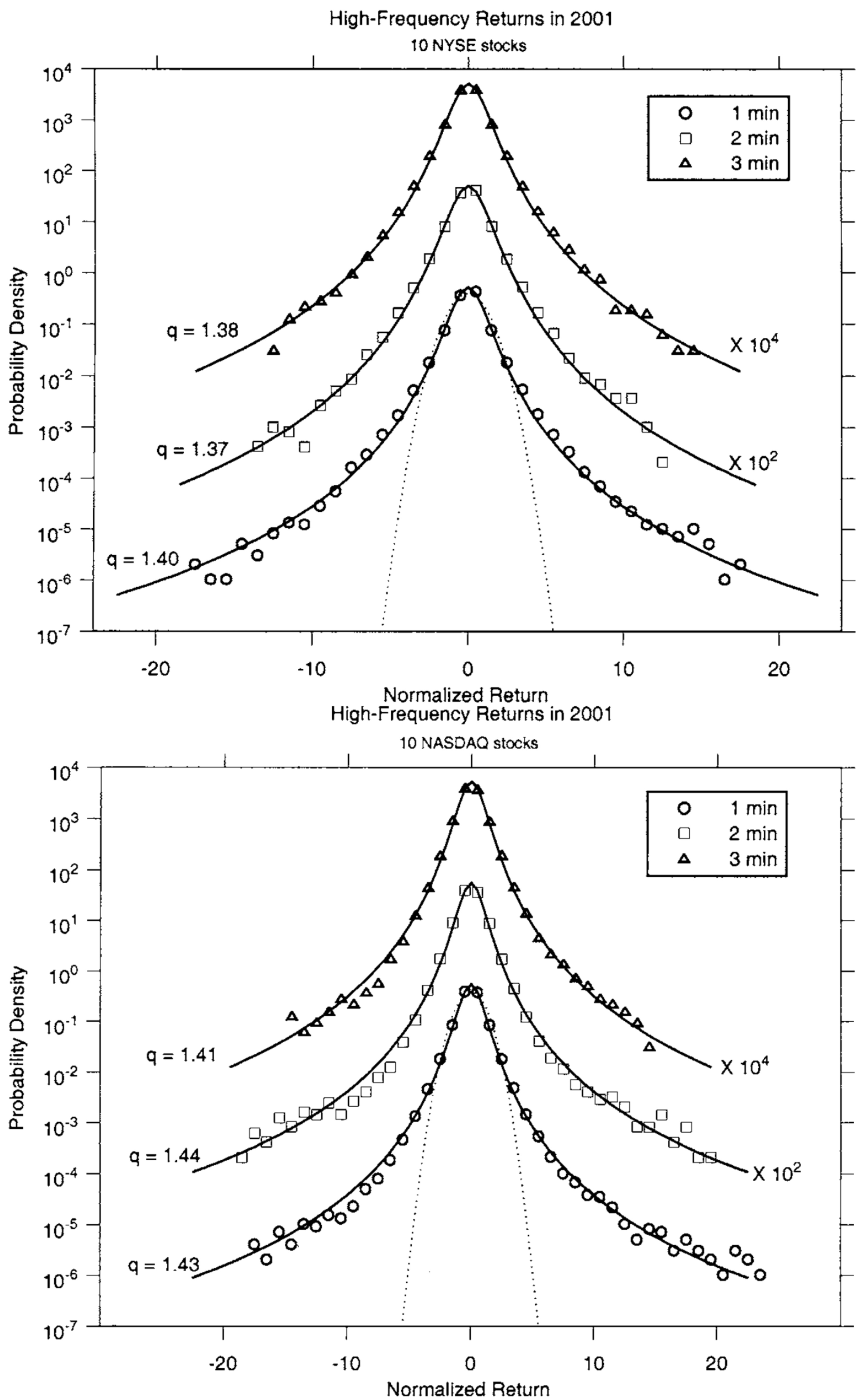
Returns do not depend on the specific currency of the prices and fluctuate around zero; in addition to that, their definition cancels systematic inflation. The distribution of returns usefully characterizes the price fluctuations. See an illustration in Figure 1, from [103] (see also [104,118]). The amounts of the corresponding transactions are currently referred to as volumes: see, for example, Figure 2.
2.2. Volatilities
The volatility characterizes the size (standard deviation) of the fluctuations of returns. The volatility smile characterizes the correction of empirical volatilities with regard to a Gaussian-based expectation: see an illustration in Figure 3 (from [103]). To be more explicit, let us assume that we are handling the following Gaussian distribution , where characterizes univocally the volatility. To discuss the probability distribution of quantities such as , Queiros introduced [108] the q-log normal probability function:
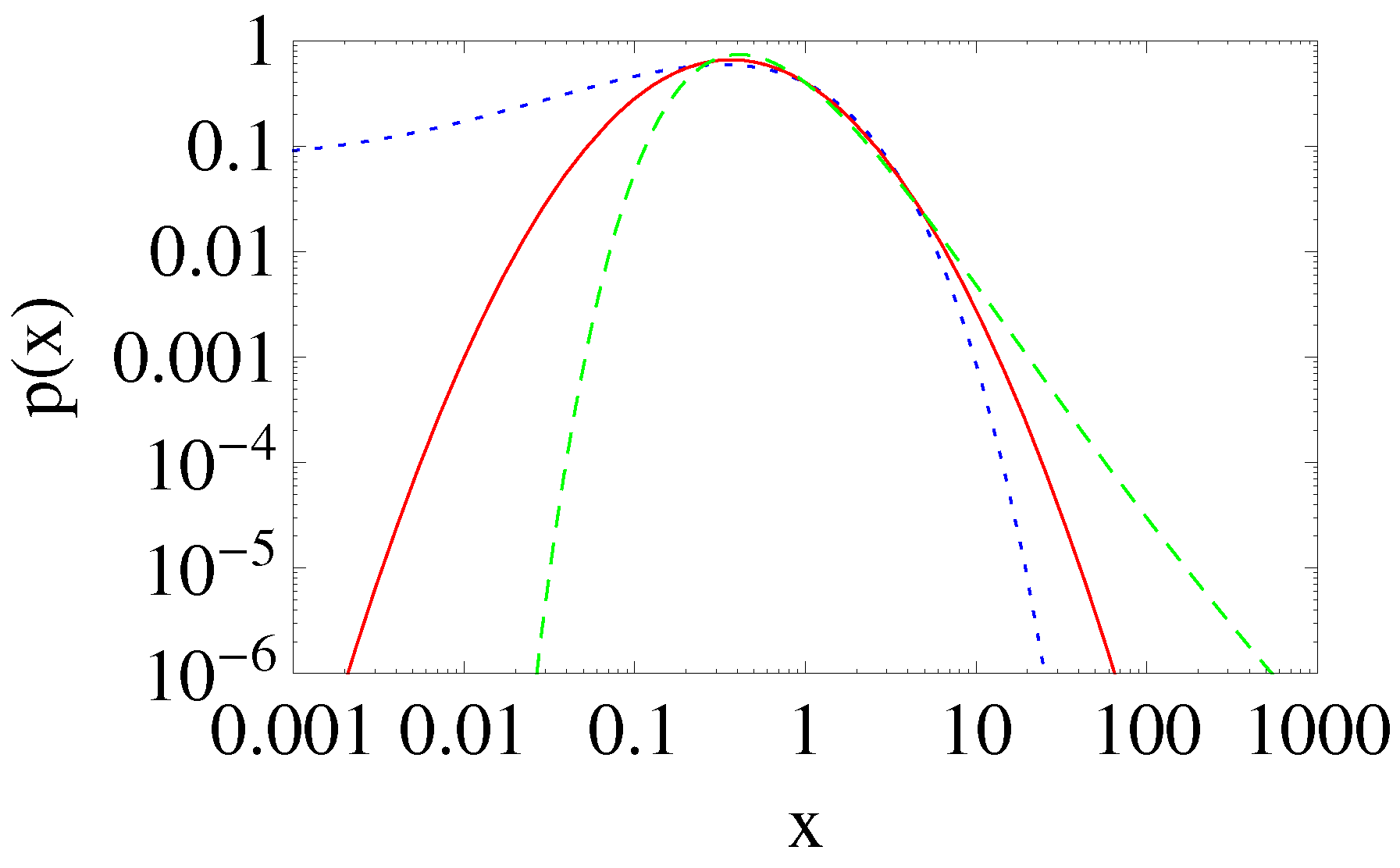
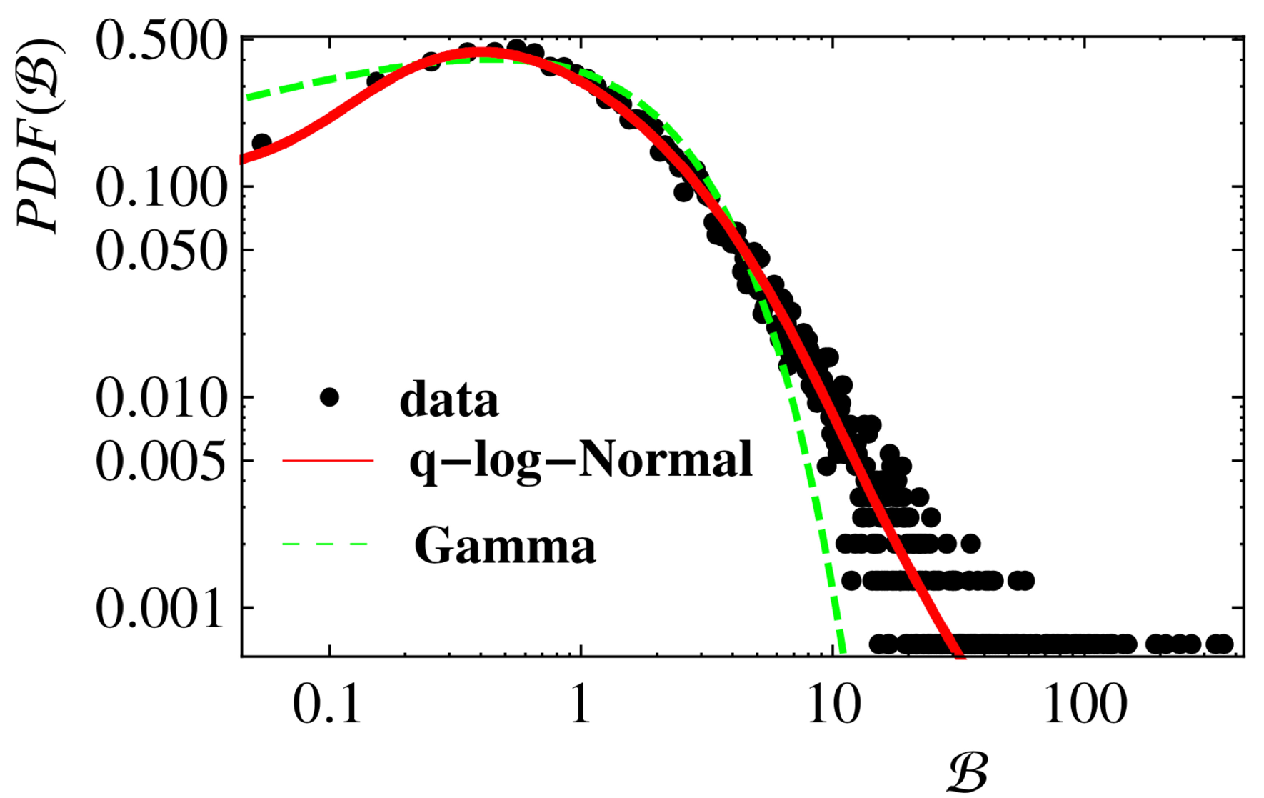
where is a normalizing factor and are parameters. The particular case corresponds to the standard log-normal function. See Figure 4 for illustrative examples of this function. See also Figure 5 for a real financial application.
2.3. Inter-Occurrence Times
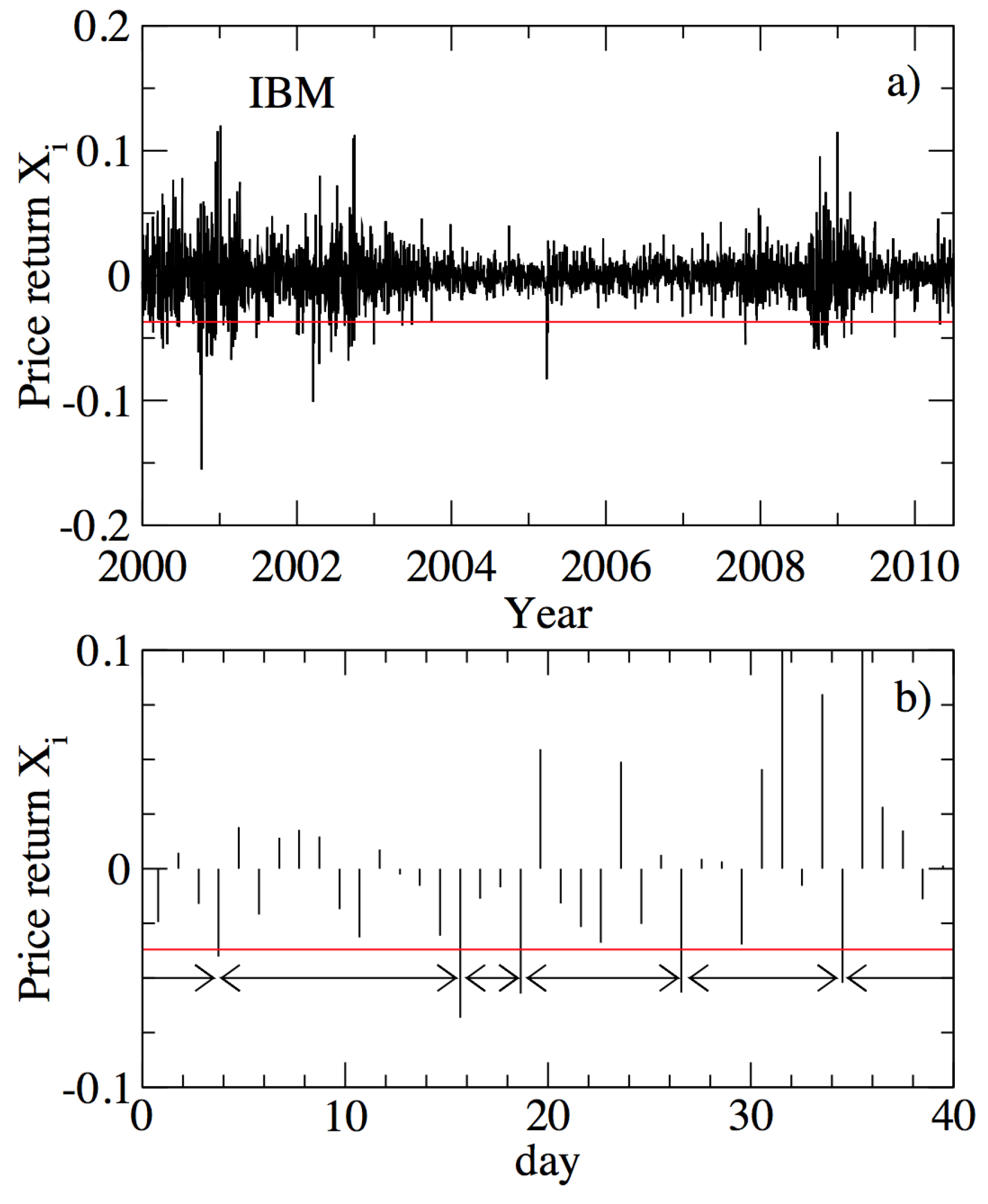
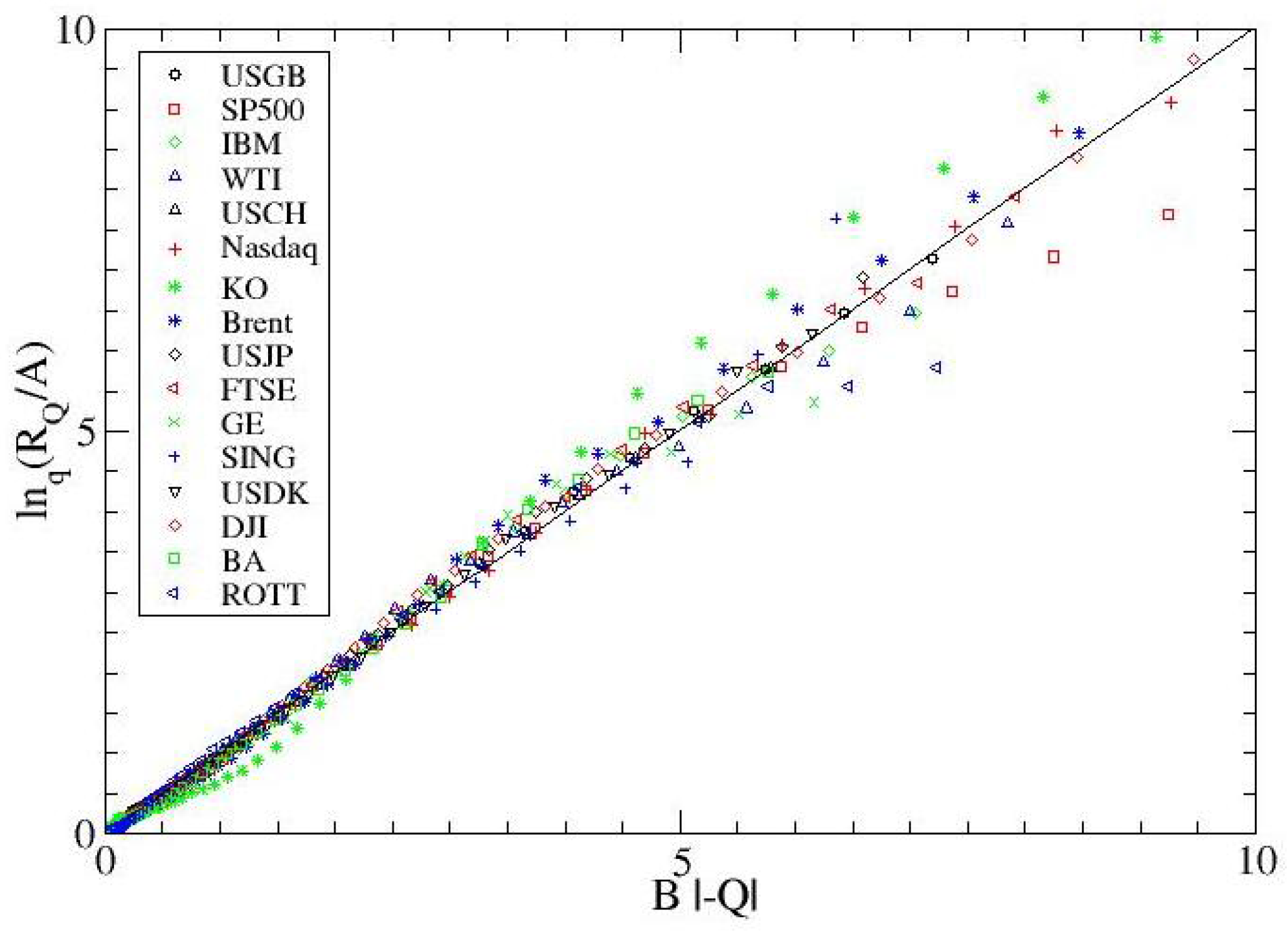
We can see in Figure 6 two typical time series of price returns, together with a chosen threshold , which corresponds to an average inter-occurrence time [106,107]. The quantity monotonically increases with in each one of the examples shown in Figure 7 and Figure 8. For a fixed value of , we verify that , with:
See the illustrations in Figure 9 and Figure 10. The fact that we have analytically enables us to straightforwardly obtain an explicit expression for the risk function , which is defined as the probability of having once again a fluctuation larger than within an interval at time t after the last large fluctuation. It can be shown [106,109] that:
with . See Figure 11.
2.4. Wealth
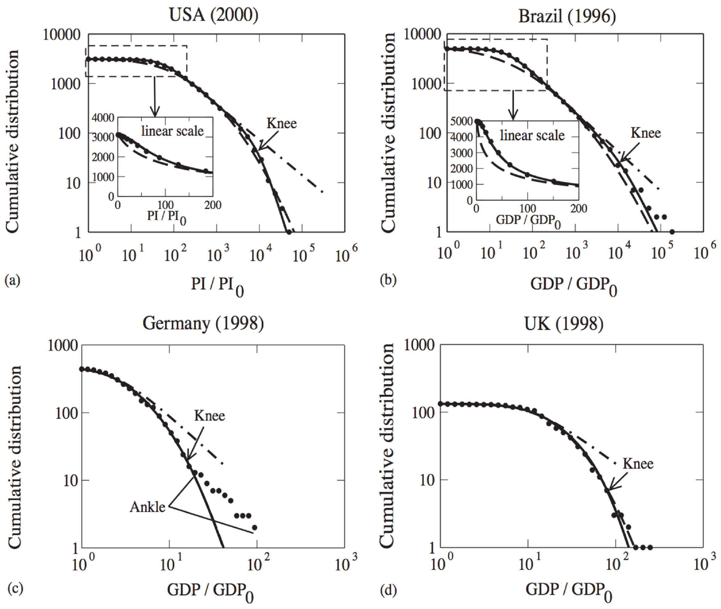
Wealth inequality within a given country is a classical and most important matter, which can be characterized within q-statistics as shown in [105]: see Figure 12 and Figure 13. The larger the index is, the larger the inequality. As we verify, the U.K. and Germany are more egalitarian countries than the U.S. and Brazil. In addition to that, inequality appears to increase in the U.S. and Brazil, at least during the years indicated in the plots.
3. Conclusions and Perspectives
We have described a variety of financial and economic properties with a plethora of q-indices, such as . For a given system, how many independent indices should we expect? The full answer to this question remains up to now elusive. It seems however that only a few of them are essentially independent, all of the others being (possibly simple) functions of those few. Such an algebraic structure was first advanced and described in [119] and has been successfully verified in the solar wind [53] (see also [6] and the references therein) and elsewhere; it has recently been generalized [120,121] and related to the Moebius group. The central elements of these algebraic structures appear to constitute what is currently referred to in the literature as q-triplets [122]. The clarification and possible verification of such structures constitutes nowadays an important open question, whose further study would surely be most useful.
Another crucial question concerns the analytic calculation from first principles of some or all of the above q-indices. This is in principle possible (as illustrated in [63,64,65,66]), but it demands the complete knowledge of the microscopic model of the specific class of the complex system. For the full set of the q-indices shown in the present overview, such models are not available, even if they would be very welcome.
Let us finally emphasize that many other statistical approaches exist for the quantities focused on in the present overview. However, as announced in the title of this paper, this is out of the present scope. The present paper is one among various others belonging to the same Special Issue of the journal Entropy. The entire set of articles is expected to enable comparisons between these many approaches.
Acknowledgments
I thank C. Anteneodo, E.P. Borges, L. Borland, E.M.F. Curado, F.D. Nobre, R. Osorio, A.R. Plastino, S.M.D. Queiros, G. Ruiz, and U. Tirnakli for longstanding fruitful conversations. I thank especially J. Ludescher for authorizing me to use, in the present review, our unpublished figures of [107]. The financial support from CNPq and FAPERJ (Conselho Nacional de Desenvolvimento Cientifico e Tecnologico, and Fundacao de Amparo a Pesquisa do Rio de Janeiro, Brazilian funding agencies) and from the John Templeton Foundation (U.S.) are also gratefully acknowledged.
Conflicts of Interest
The author declares no conflict of interest.
References
- Penrose, O. Foundations of Statistical Mechanics: A Deductive Treatment; Pergamon: Oxford, UK, 1970; p. 167. [Google Scholar]
- Tsallis, C. Possible generalization of Boltzmann–Gibbs statistics. J. Stat. Phys. 1988, 53, 479–487. [Google Scholar]
- Curado, E.M.F.; Tsallis, C. Generalized statistical mechanics: Connection with thermodynamics. J. Phys. A 1991, 24, L69–L72. [Google Scholar]
- Tsallis, C.; Mendes, R.S.; Plastino, A.R. The role of constraints within generalized nonextensive statistics. Physica A 1998, 261, 534–554. [Google Scholar]
- Gell-Mann, M.; Tsallis, C. (Eds.) Nonextensive Entropy-Interdisciplinary Applications; Oxford University Press: New York, NY, USA, 2004. [Google Scholar]
- Tsallis, C. Introduction to Nonextensive Statistical Mechanics-Approaching a Complex World; Springer: New York, NY, USA, 2009. [Google Scholar]
- Muskat, M. The Flow of Homogeneous Fluids through Porous Media; McGraw-Hill: New York, NY, USA, 1937. [Google Scholar]
- Frank, T.D. Nonlinear Fokker–Planck Equations: Fundamentals and Applications; Series Synergetics; Springer: Berlin, Germany, 2005. [Google Scholar]
- Tsallis, C.; Bukman, D.J. Anomalous diffusion in the presence of external forces: Exact time-dependent solutions and their thermostatistical basis. Phys. Rev. E 1996, 54, R2197–R2200. [Google Scholar]
- Combe, G.; Richefeu, V.; Stasiak, M.; Atman, A.P.F. Experimental validation of nonextensive scaling law in confined granular media. Phys. Rev. Lett. 2015, 115, 238301. [Google Scholar]
- Plastino, A.R.; Plastino, A. Non-extensive statistical mechanics and generalized Fokker–Planck equation. Physica A 1995, 222, 347–354. [Google Scholar]
- Nonextensive Statistical Mechanics and Thermodynamics. Available online: http://tsallis.cat.cbpf.br/biblio.htm (accessed on 29 August 2017).
- Anteneodo, C.; Tsallis, C. Breakdown of exponential sensitivity to initial conditions: Role of the range of interactions. Phys. Rev. Lett. 1998, 80, 5313–5316. [Google Scholar]
- Rapisarda, A.; Pluchino, A. Nonextensive thermodynamics and glassy behavior. Europhys. News 2005, 36, 202–206. [Google Scholar]
- Chavanis, P.-H.; Campa, A. Inhomogeneous Tsallis distributions in the HMF model. Eur. Phys. J. B 2010, 76, 581–611. [Google Scholar]
- Cirto, L.J.L.; Assis, V.R.V.; Tsallis, C. Influence of the interaction range on the thermostatistics of a classical many-body system. Physica A 2014, 393, 286–296. [Google Scholar]
- Christodoulidi, H.; Tsallis, C.; Bountis, T. Fermi–Pasta–Ulam model with long-range interactions: Dynamics and thermostatistics. EPL 2014, 108, 40006. [Google Scholar]
- Christodoulidi, H.; Bountis, T.; Tsallis, C.; Drossos, L. Dynamics and Statistics of the Fermi–Pasta–Ulam β–model with different ranges of particle interactions. JSTAT 2016, 123206. [Google Scholar]
- Bagchi, D.; Tsallis, C. Sensitivity to initial conditions of d-dimensional long-range-interacting quartic Fermi–Pasta–Ulam model: Universal scaling. Phys. Rev. E 2016, 93, 062213. [Google Scholar]
- Bagchi, D.; Tsallis, C. Long-ranged Fermi–Pasta–Ulam systems in thermal contact: Crossover from q-statistics to Boltzmann–Gibbs statistics. Phys. Lett. A 2017, 381, 1123–1128. [Google Scholar]
- Lucena, L.S.; da Silva, L.R.; Tsallis, C. Departure from Boltzmann–Gibbs statistics makes the hydrogen-atom specific heat a computable quantity. Phys. Rev. E 1995, 51, 6247–6249. [Google Scholar]
- Nobre, F.D.; Tsallis, C. Infinite-range Ising ferromagnet-thermodynamic limit within generalized statistical mechanics. Physica A 1995, 213, 337–356. [Google Scholar]
- Caride, A.O.; Tsallis, C.; Zanette, S.I. Criticality of the anisotropic quantum Heisenberg model on a self-dual hierarchical lattice. Phys. Rev. Lett. 1983, 51, 145–147. [Google Scholar]
- Miritello, G.; Pluchino, A.; Rapisarda, A. Central limit behavior in the Kuramoto model at the ‘edge of chaos’. Physica A 2009, 388, 4818–4826. [Google Scholar]
- Tirnakli, U.; Tsallis, C.; Lyra, M.L. Circular-like maps: sensitivity to the initial conditions, multifractality and nonextensivity. Eur. Phys. J. B 1999, 11, 309–315. [Google Scholar]
- Baldovin, F.; Robledo, A. Universal renormalization-group dynamics at the onset of chaos in logistic maps and nonextensive statistical mechanics. Phys. Rev. E 2002, 66, R045104. [Google Scholar]
- Baldovin, F.; Robledo, A. Nonextensive Pesin identity. Exact renormalization group analytical results for the dynamics at the edge of chaos of the logistic map. Phys. Rev. E 2004, 69, R045202. [Google Scholar]
- Mayoral, E.; Robledo, A. Tsallis’ q index and Mori’s q phase transitions at edge of chaos. Phys. Rev. E 2005, 72, 026209. [Google Scholar]
- Tirnakli, U.; Tsallis, C.; Beck, C. A closer look at time averages of the logistic map at the edge of chaos. Phys. Rev. E 2009, 79, 056209. [Google Scholar]
- Luque, B.; Lacasa, L.; Robledo, A. Feigenbaum graphs at the onset of chaos. Phys. Lett. A 2012, 376, 3625. [Google Scholar] [CrossRef]
- Tirnakli, U.; Borges, E.P. The standard map: From Boltzmann–Gibbs statistics to Tsallis statistics. Nat. Sci. Rep. 2016, 6, 23644. [Google Scholar]
- Douglas, P.; Bergamini, S.; Renzoni, F. Tunable Tsallis Distributions in Dissipative Optical Lattices. Phys. Rev. Lett. 2006, 96, 110601. [Google Scholar]
- Bagci, G.B.; Tirnakli, U. Self-organization in dissipative optical lattices. Chaos 2009, 19, 033113. [Google Scholar]
- Lutz, E.; Renzoni, F. Beyond Boltzmann–Gibbs statistical mechanics in optical lattices. Nat. Phys. 2013, 9, 615–619. [Google Scholar]
- Liu, B.; Goree, J. Superdiffusion and non-Gaussian statistics in a driven-dissipative 2D dusty plasma. Phys. Rev. Lett. 2008, 100, 055003. [Google Scholar]
- Bouzit, O.; Gougam, L.A.; Tribeche, M. Screening and sheath formation in a nonequilibrium mixed Cairns-Tsallis electron distribution. Phys. Plasmas 2015, 22, 052112. [Google Scholar]
- DeVoe, R.G. Power-law distributions for a trapped ion interacting with a classical buffer gas. Phys. Rev. Lett. 2009, 102, 063001. [Google Scholar]
- Pickup, R.M.; Cywinski, R.; Pappas, C.; Farago, B.; Fouquet, P. Generalized spin glass relaxation. Phys. Rev. Lett. 2009, 102, 097202. [Google Scholar]
- Tsallis, C.; de Souza, A.M.C.; Maynard, R. Derivation of Lévy-type anomalous superdiffusion from generalized statistical mechanics. In Lévy Flights and Related Topics in Physics; Shlesinger, M.F., Zaslavsky, G.M., Frisch, U., Eds.; Springer: Berlin, Germany, 1995; p. 269. [Google Scholar]
- Tsallis, C.; Levy, S.V.F.; de Souza, A.M.C.; Maynard, R. Statistical-mechanical foundation of the ubiquity of Levy distributions in nature. Phys. Rev. Lett. 1995, 75, 3589–3593. [Google Scholar]
- CMS Collaboration. Transverse-momentum and pseudorapidity distributions of charged hadrons in pp collisions at and 2.36 TeV. J. High Energy Phys. 2010, 2, 41. [Google Scholar] [CrossRef]
- CMS Collaboration. Transverse-momentum and pseudorapidity distributions of charged hadrons in pp collisions at TeV. Phys. Rev. Lett. 2010, 105, 022002. [Google Scholar]
- Marques, L.; Andrade, E., II; Deppman, A. Nonextensivity of hadronic systems. Phys. Rev. D 2013, 87, 114022. [Google Scholar]
- Marques, L.; Cleymans, J.; Deppman, A. Description of high-energy pp collisions using Tsallis thermodynamics: Transverse momentum and rapidity distributions. Phys. Rev. D 2015, 91, 054025. [Google Scholar]
- Tsallis, C.; Arenas, Z.G. Nonextensive statistical mechanics and high energy physics. EPJ 2014, 71, 00132. [Google Scholar]
- ALICE Collaboration. K*(892)0 and Φ(1020) meson production at high transverse momentum in pp and Pb-Pb collisions at TeV. Phys. Rev. C 2017, 95, 064606. [Google Scholar]
- Oliveira, H.P.; Soares, I.D. Dynamics of black hole formation: Evidence for nonextensivity. Phys. Rev. D 2005, 71, 124034. [Google Scholar]
- Komatsu, N.; Kimura, S. Entropic cosmology for a generalized black-hole entropy. Phys. Rev. D 2013, 88, 083534. [Google Scholar]
- Silva, V.H.C.; Aquilanti, V.; de Oliveira, H.C.B.; Mundim, K.C. Uniform description of non-Arrhenius temperature dependence of reaction rates, and a heuristic criterion for quantum tunneling vs. classical non-extensive distribution. Chem. Phys. Lett. 2013, 590, 201–207. [Google Scholar]
- Antonopoulos, C.G.; Michas, G.; Vallianatos, F.; Bountis, T. Evidence of q-exponential statistics in Greek seismicity. Physica A 2014, 409, 71–77. [Google Scholar]
- Upadhyaya, A.; Rieu, J.-P.; Glazier, J.A.; Sawada, Y. Anomalous diffusion and non-Gaussian velocity distribution of Hydra cells in cellular aggregates. Physica A 2001, 293, 549–558. [Google Scholar]
- Bogachev, M.I.; Kayumov, A.R.; Bunde, A. Universal internucleotide statistics in full genomes: A footprint of the DNA structure and packaging? PLoS ONE 2014, 9, e112534. [Google Scholar]
- Burlaga, L.F.; Vinas, A.F. Triangle for the entropic index q of non-extensive statistical mechanics observed by Voyager 1 in the distant heliosphere. Physica A 2005, 356, 375–384. [Google Scholar]
- Burlaga, L.F.; Ness, N.F. Magnetic field strength fluctuations and the q-triplet in the heliosheath: Voyager 2 observations from 91.0 to 94.2 AU at latitude 30° S. Astrophys. J. 2013, 765, 35. [Google Scholar]
- Moyano, L.G.; Tsallis, C.; Gell-Mann, M. Numerical indications of a q-generalised central limit theorem. Europhys. Lett. 2006, 73, 813–819. [Google Scholar]
- Thistleton, W.J.; Marsh, J.A.; Nelson, K.P.; Tsallis, C. q-Gaussian approximants mimic non-extensive statistical-mechanical expectation for many-body probabilistic model with long-range correlations. Cent. Eur. J. Phys. 2009, 7, 387–394. [Google Scholar]
- Chavanis, P.-H. Nonlinear mean field Fokker–Planck equations. Application to the chemotaxis of biological population. Eur. Phys. J. B 2008, 62, 179–208. [Google Scholar]
- Umarov, S.; Tsallis, C.; Steinberg, S. On a q-central limit theorem consistent with nonextensive statistical mechanics. J. Math. 2008, 76, 307–328. [Google Scholar]
- Umarov, S.; Tsallis, C.; Gell-Mann, M.; Steinberg, S. Generalization of symmetric α-stable Lévy distributions for q > 1. Math. Phys. 2010, 51, 033502. [Google Scholar]
- Nelson, K.P.; Umarov, S. Nonlinear statistical coupling. Physica A 2010, 389, 2157–2163. [Google Scholar]
- Hanel, R.; Thurner, S.; Tsallis, C. Limit distributions of scale-invariant probabilistic models of correlated random variables with the q-Gaussian as an explicit example. Eur. Phys. J. B 2009, 72, 263–268. [Google Scholar]
- Umarov, S.; Tsallis, C. The limit distribution in the q-CLT for q ≥ 1 is unique and can not have a compact support. J. Phys. A 2016, 49, 415204. [Google Scholar]
- Andrade, J.S., Jr.; da Silva, G.F.T.; Moreira, A.A.; Nobre, F.D.; Curado, E.M.F. Thermostatistics of overdamped motion of interacting particles. Phys. Rev. Lett. 2010, 105, 260601. [Google Scholar]
- Vieira, C.M.; Carmona, H.A.; Andrade, J.S., Jr.; Moreira, A.A. General continuum approach for dissipative systems of repulsive particles. Phys. Rev. E 2016, 93, 060103(R). [Google Scholar]
- Caruso, F.; Tsallis, C. Nonadditive entropy reconciles the area law in quantum systems with classical thermodynamics. Phys. Rev. E 2008, 78, 021102. [Google Scholar]
- Carrasco, J.A.; Finkel, F.; Gonzalez-Lopez, A.; Rodriguez, M.A.; Tempesta, P. Generalized isotropic Lipkin-Meshkov-Glick models: Ground state entanglement and quantum entropies. J. Stat. Mech. 2016, 2016, 033114. [Google Scholar]
- Weinstein, Y.S.; Lloyd, S.; Tsallis, C. Border between between regular and chaotic quantum dynamics. Phys. Rev. Lett. 2002, 89, 214101. [Google Scholar]
- Betzler, A.S.; Borges, E.P. Nonextensive distributions of asteroid rotation periods and diameters. Astron. Astrophys. 2012, 539, A158. [Google Scholar] [CrossRef]
- Betzler, A.S.; Borges, E.P. Nonextensive statistical analysis of meteor showers and lunar flashes. Mon. Not. R. Astron. Soc. 2015, 447, 765–771. [Google Scholar]
- Li, Y.; Li, N.; Tirnakli, U.; Li, B.; Tsallis, C. Thermal conductance of the coupled-rotator chain: Influence of temperature and size. EPL 2017, 117, 60004. [Google Scholar]
- Nivanen, L.; Le Mehaute, A.; Wang, Q.A. Generalized algebra within a nonextensive statistics. Rep. Math. Phys. 2003, 54, 437–444. [Google Scholar]
- Borges, E.P. A possible deformed algebra and calculus inspired in nonextensive thermostatistics. Physica A 2004, 340, 95–101. [Google Scholar]
- Tempesta, P. Group entropies, correlation laws, and zeta functions. Phys. Rev. E 2011, 84, 021121. [Google Scholar]
- Ruiz, G.; Tsallis, C. Reply to comment on “towards a large deviation theory for strongly correlated systems”. Phys. Lett. A 2013, 377, 491–495. [Google Scholar]
- Jauregui, M.; Tsallis, C. New representations of π and Dirac delta using the nonextensive- statistical-mechanics q-exponential function. Math. Phys. 2010, 51, 063304. [Google Scholar]
- Sicuro, G.; Tsallis, C. q-Generalized representation of the d-dimensional Dirac delta and q-Fourier transform. Phys. Lett. A 2017, 381, 2583–2587. [Google Scholar]
- Nobre, F.D.; Rego-Monteiro, M.A.; Tsallis, C. Nonlinear relativistic and quantum equations with a common type of solution. Phys. Rev. Lett. 2011, 106, 140601. [Google Scholar]
- Costa Filho, R.N.; Almeida, M.P.; Farias, G.A.; Andrade, J.S., Jr. Displacement operator for quantum systems with position-dependent mass. Phys. Rev. A 2011, 84, 050102(R). [Google Scholar]
- Mazharimousavi, S.H. Revisiting the displacement operator for quantum systems with position-dependent mass. Phys. Rev. A 2010, 85, 034102. [Google Scholar]
- Nobre, F.D.; Rego-Monteiro, M.A.; Tsallis, C. A generalized nonlinear Schroedinger equation: Classical field-theoretic approach. Europhys. Lett. 2012, 97, 41001. [Google Scholar]
- Rego-Monteiro, M.A.; Nobre, F.D. Nonlinear quantum equations: Classical field theory. J. Math. Phys. 2013, 54, 103302. [Google Scholar]
- Rego-Monteiro, M.A.; Nobre, F.D. Classical field theory for a non-Hermitian Schroedinger equation with position-dependent masses. Phys. Rev. A 2013, 88, 032105. [Google Scholar]
- Costa Filho, R.N.; Alencar, G.; Skagerstam, B.-S.; Andrade, J.S., Jr. Morse potential derived from first principles. Europhys. Lett. 2013, 101, 10009. [Google Scholar]
- Toranzo, I.V.; Plastino, A.R.; Dehesa, J.S.; Plastino, A. Quasi-stationary states of the NRT nonlinear Schroedinger equation. Physica A 2013, 392, 3945–3951. [Google Scholar]
- Curilef, S.; Plastino, A.R.; Plastino, A. Tsallis’ maximum entropy ansatz leading to exact analytical time dependent wave packet solutions of a nonlinear Schroedinger equation. Physica A 2013, 392, 2631–2642. [Google Scholar]
- Plastino, A.R.; Tsallis, C. Nonlinear Schroedinger equation in the presence of uniform acceleration. J. Math. Phys. 2013, 54, 041505. [Google Scholar]
- Plastino, A.R.; Souza, A.M.C.; Nobre, F.D.; Tsallis, C. Stationary and uniformly accelerated states in nonlinear quantum mechanics. Phys. Rev. A 2014, 90, 062134. [Google Scholar]
- Pennini, F.; Plastino, A.R.; Plastino, A. Pilot wave approach to the NRT nonlinear Schroedinger equation. Physica A 2014, 403, 195–205. [Google Scholar]
- Da Costa, B.G.; Borges, E.P. Generalized space and linear momentum operators in quantum mechanics. J. Math. Phys. 2014, 55, 062105. [Google Scholar]
- Nobre, F.D.; Rego-Monteiro, M.A. Non-Hermitian PT symmetric Hamiltonian with position-dependent masses: Associated Schroedinger equation and finite-norm solutions. Braz. J. Phys. 2015, 45, 79–88. [Google Scholar]
- Plastino, A.; Rocca, M.C. From the hypergeometric differential equation to a non-linear Schroedinger one. Phys. Lett. A 2015, 379, 2690–2693. [Google Scholar]
- Alves, L.G.A.; Ribeiro, H.V.; Santos, M.A.F.; Mendes, R.S.; Lenzi, E.K. Solutions for a q-generalized Schroedinger equation of entangled interacting particles. Physica A 2015, 429, 35–44. [Google Scholar]
- Plastino, A.R.; Tsallis, C. Dissipative effects in nonlinear Klein–Gordon dynamics. EPL 2016, 113, 50005. [Google Scholar]
- Plastino, A.; Rocca, M.C. Hypergeometric connotations of quantum equations. Physica A 2016, 450, 435–443. [Google Scholar]
- Bountis, T.; Nobre, F.D. Travelling-wave and separated variable solutions of a nonlinear Schroedinger equation. J. Math. Phys. 2016, 57, 082106. [Google Scholar]
- Nobre, F.D.; Plastino, A.R. A family of nonlinear Schroedinger equations admitting q-plane wave. Phys. Lett. A 2017, 381, 2457–2462. [Google Scholar]
- Capurro, A.; Diambra, L.; Lorenzo, D.; Macadar, O.; Martin, M.T.; Mostaccio, C.; Plastino, A.; Rofman, E.; Torres, M.E.; Velluti, J. Tsallis entropy and cortical dynamics: The analysis of EEG signals. Physica A 1998, 257, 149–155. [Google Scholar]
- Mohanalin, J.; Beenamol; Kalra, P.K.; Kumar, N. A novel automatic microcalcification detection technique using Tsallis entropy and a type II fuzzy index. Comput. Math. Appl. 2010, 60, 2426–2432. [Google Scholar]
- Soares, D.J.B.; Tsallis, C.; Mariz, A.M.; Silva, L.R. Preferential attachment growth model and nonextensive statistical mechanics. EPL 2005, 70, 70–76. [Google Scholar]
- Thurner, S.; Tsallis, C. Nonextensive aspects of self-organized scale-free gas-like networks. Europhys. Lett. 2005, 72, 197–203. [Google Scholar]
- Brito, S.G.A.; da Silva, L.R.; Tsallis, C. Role of dimensionality in complex networks. Nat. Sci. Rep. 2016, 6, 27992. [Google Scholar]
- Borland, L. Closed form option pricing formulas based on a non-Gaussian stock price model with statistical feedback. Phys. Rev. Lett. 2002, 89, 098701. [Google Scholar]
- Tsallis, C.; Anteneodo, C.; Borland, L.; Osorio, R. Nonextensive statistical mechanics and economics. Physica A 2003, 324, 89–100. [Google Scholar]
- Osorio, R.; Borland, L.; Tsallis, C. Distributions of high-frequency stock-market observables. In Nonextensive Entropy-Interdisciplinary Applications; Gell-Mann, M., Tsallis, C., Eds.; Oxford University Press: New York, NY, USA, 2004. [Google Scholar]
- Borges, E.P. Empirical nonextensive laws for the county distribution of total personal income and gross domestic product. Physica A 2004, 334, 255–266. [Google Scholar]
- Ludescher, J.; Tsallis, C.; Bunde, A. Universal behaviour of inter-occurrence times between losses in financial markets: An analytical description. Europhys. Lett. 2011, 95, 68002. [Google Scholar]
- Ludescher, J.; Institut fur Theoretische Physik, Justus-Liebig-Universitat, Giessen, Germany; Tsallis, C.; Centro Brasileiro de Pesquisas Físicas and National Institute of Science and Technology for Complex Systems, Rio de Janeiro, Brazil. Private Communications, 2011.
- Queiros, S.M.D. On generalisations of the log-Normal distribution by means of a new product definition in the Kapteyn process. Physica A 2012, 391, 3594–3606. [Google Scholar]
- Bogachev, M.I.; Eichner, J.F.; Bunde, A. Effect of nonlinear correlations on the statistics of return intervals in multifractal data sets. Phys. Rev. Lett. 2007, 99, 240601. [Google Scholar]
- Ludescher, J.; Bunde, A. Universal behavior of the inter-occurrence times between losses in financial markets: Independence of the time resolution. Phys. Rev. 2014, 90, 062809. [Google Scholar]
- Perello, J.; Gutierrez-Roig, M.; Masoliver, J. Scaling properties and universality of first-passage-time probabilities in financial markets. Phys. Rev. E 2011, 84, 066110. [Google Scholar]
- Ruseckas, J.; Kaulakys, B.; Gontis, V. Herding model and 1/f noise. EPL 2011, 96, 60007. [Google Scholar]
- Ruseckas, J.; Gontis, V.; Kaulakys, B. Nonextensive statistical mechanics distributions and dynamics of financial observables from the nonlinear stochastic differential equations. Adv. Complex Syst. 2012, 15, 1250073. [Google Scholar]
- Gontis, V.; Kononovicius, A. A consentaneous agent based and stochastic model of the financial markets. PLoS ONE 2014, 9, e102201. [Google Scholar]
- Biondo, A.E.; Pluchino, A.; Rapisarda, A. Modeling financial markets by self-organized criticality. Phys. Rev. E 2015, 92, 042814. [Google Scholar]
- Biondo, A.E.; Pluchino, A.; Rapisarda, A. Order book, financial markets, and self-organized criticality. Chaos Solitons Fractals 2016, 88, 196–208. [Google Scholar]
- Biondo, A.E.; Pluchino, A.; Rapisarda, A. A multilayer approach for price dynamics in financial markets. Eur. Phys. J. Spec. Top. 2017, 226, 477–488. [Google Scholar]
- Ruiz, G.; Fernandez, A. Evidence for criticality in financial data. arXiv, 2017; arXiv:1702.06191. [Google Scholar]
- Tsallis, C.; Gell-Mann, M.; Sato, Y. Asymptotically scale-invariant occupancy of phase space makes the entropy Sq extensive. Proc. Natl. Acad. Sci. USA 2005, 102, 15377–15382. [Google Scholar]
- Tsallis, C. Generalization of the possible algebraic basis of q-triplets. Eur. Phys. J. Spec. Top. 2017, 226, 455–466. [Google Scholar]
- Tsallis, C. Statistical mechanics for complex systems: On the structure of q-triplets. In Proceedings of the 31st International Colloquium on Group Theoretical Methods in Physics, Rio de Janeiro, Brazil, 20–24 July 2016. [Google Scholar]
- Tsallis, C. Dynamical scenario for nonextensive statistical mechanics. Physica A 2004, 340, 1–10. [Google Scholar] [CrossRef]
Figure 1.
Empirical return densities (points) and q-Gaussians (solid lines) for normalized returns of the 10 top-volume stocks in the NYSE and in NASDAQ in 2001. The dotted line is a (visibly inadequate) Gaussian distribution. The 2- and 3-min curves are moved vertically for display purposes. From [103]. There exist in the literature quite a few other such examples, for other stocks and other years, with similar values of q.

Figure 2.
Empirical distributions (points) and q-exponential-like curves (solid lines) for normalized volumes of the 10 top-volume stocks in the NYSE and in the NASDAQ in 2001. The solid lines are fittings with a q-exponential multiplied by a power-law (analogous to the density of states prefactor that typically emerges for the distributions of quasi-particles in, say, condensed matter physics); from [103]. There exist in the literature quite a few other such examples, for other stocks and other years, with similar values of q and of the rest of the fitting indices.
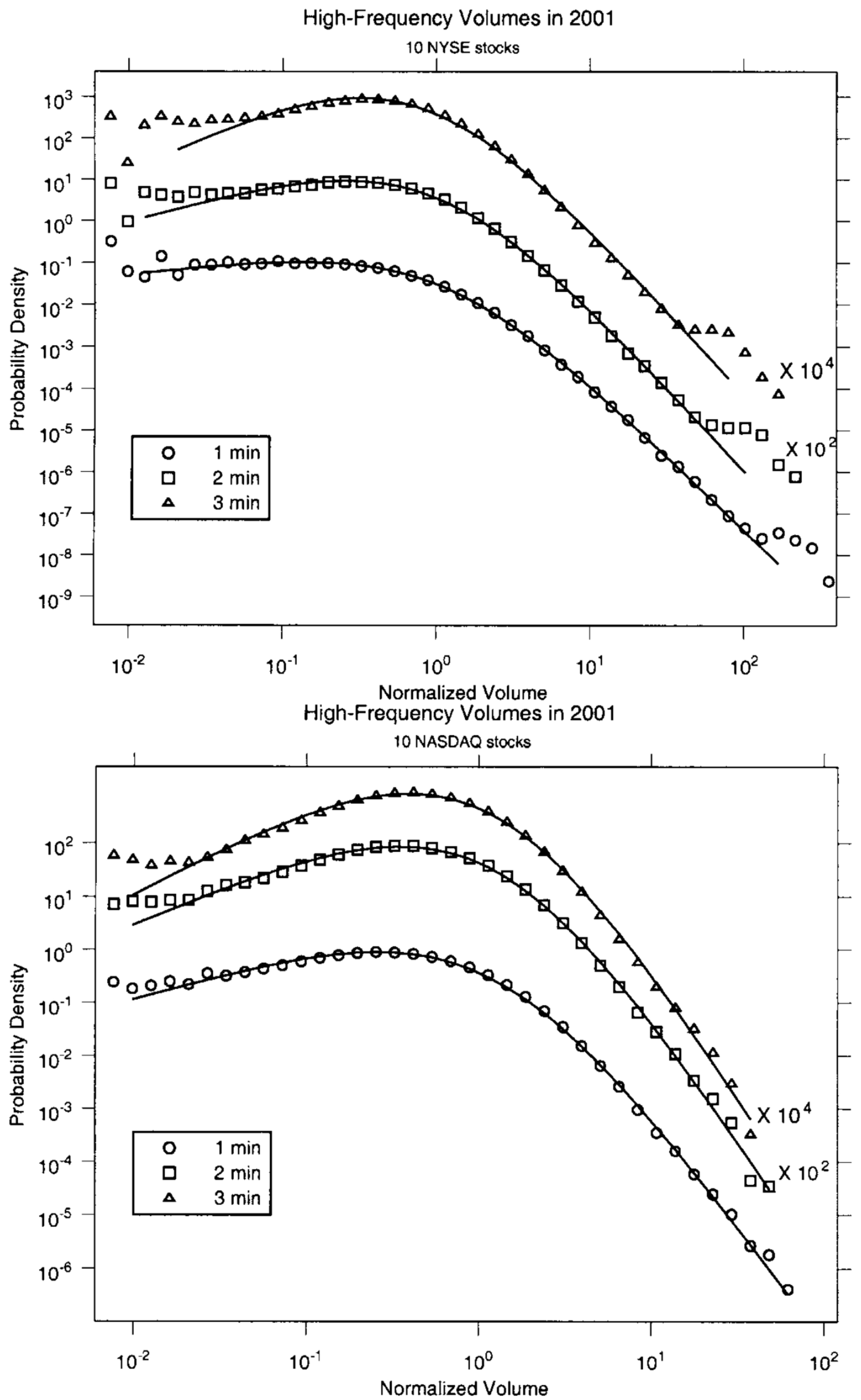
Figure 3.
Implied volatilities as a function of the strike price for call options on JY currency futures, traded on 16 May 2002, with 147 days left to expiration. In this typical example, the current price of a contract on Japanese futures is $79, and the risk-free rate of return is . Circles correspond to volatilities implied by the market, whereas triangles correspond to volatilities implied by our model with and . The dotted line is a guide to the eye. From [103].
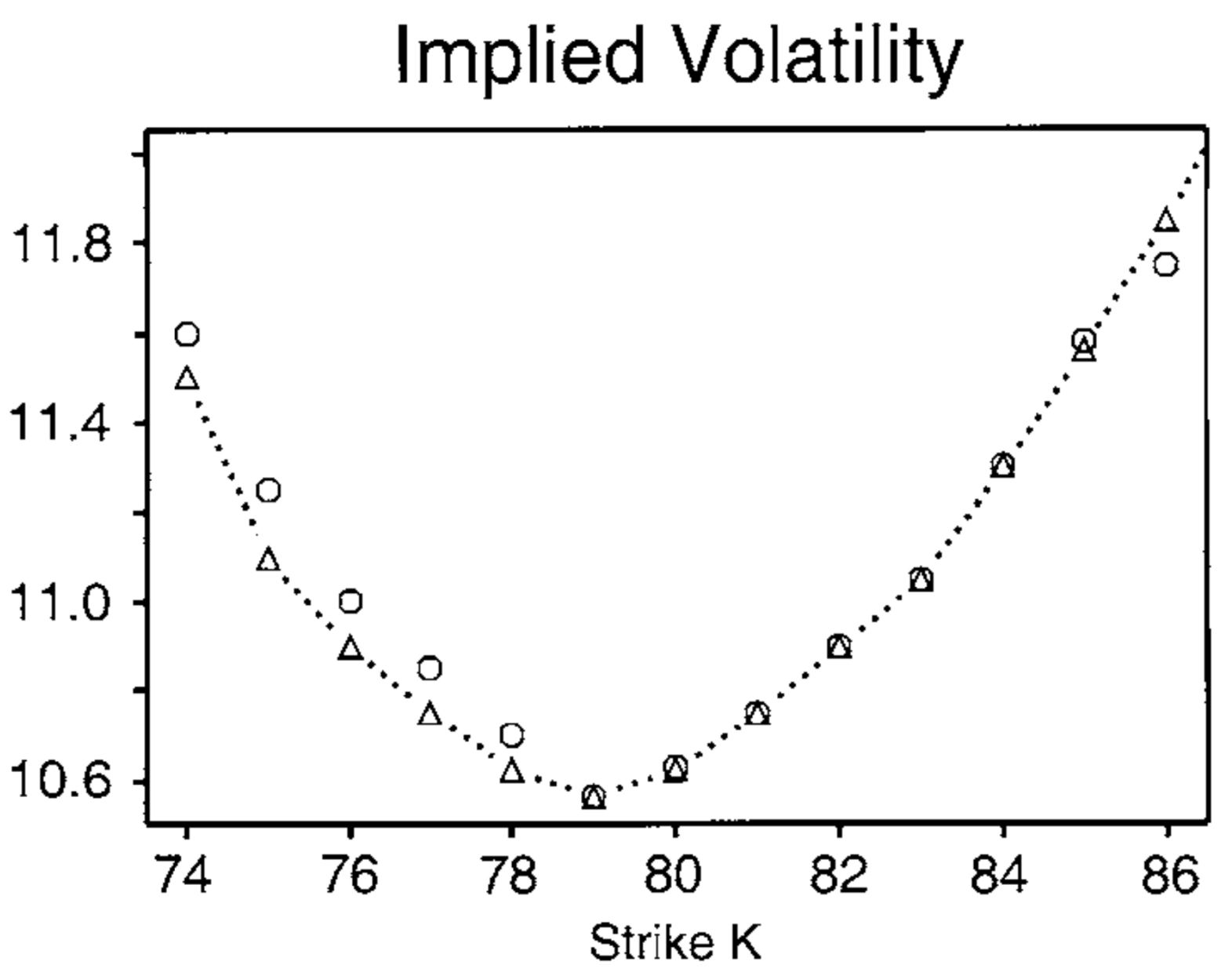
Figure 4.
Illustrations of the q-log-normal density for and : blue , red and green . From [108].
Figure 4.
Illustrations of the q-log-normal density for and : blue , red and green . From [108].

Figure 5.
Probability density function of a five-day volatility vs. . The symbols are obtained from the data, and the lines are the best fits with the Gamma distribution (dashed green) and the double-sided q-log-normal (red) with , and . For further details, see [108].
Figure 5.
Probability density function of a five-day volatility vs. . The symbols are obtained from the data, and the lines are the best fits with the Gamma distribution (dashed green) and the double-sided q-log-normal (red) with , and . For further details, see [108].

Figure 6.
Illustration of the relative daily price returns of the IBM stock between (a) January 2000 and June 2010 and (b) 27 August and 23 October 2002. The red line shows the threshold , which corresponds to an average inter-occurrence time of = 70. In (b), the inter-occurrence times are indicated by arrows. From [106].

Figure 7.
The mean inter-occurrence time vs. the absolute value of the loss threshold −Q. The continuous curves are fittings with . Top left: For the exchange rate of the U.S. Dollar against the British Pound, the index S&P500, the IBM stock and crude oil (West Texas Intermediate (WTI)), from left to right in the plot; the corresponding values for are 0.95, 0.92, 0.97, 0.927 (with and ). Similarly for the top right, bottom left and bottom right plots. From [107].
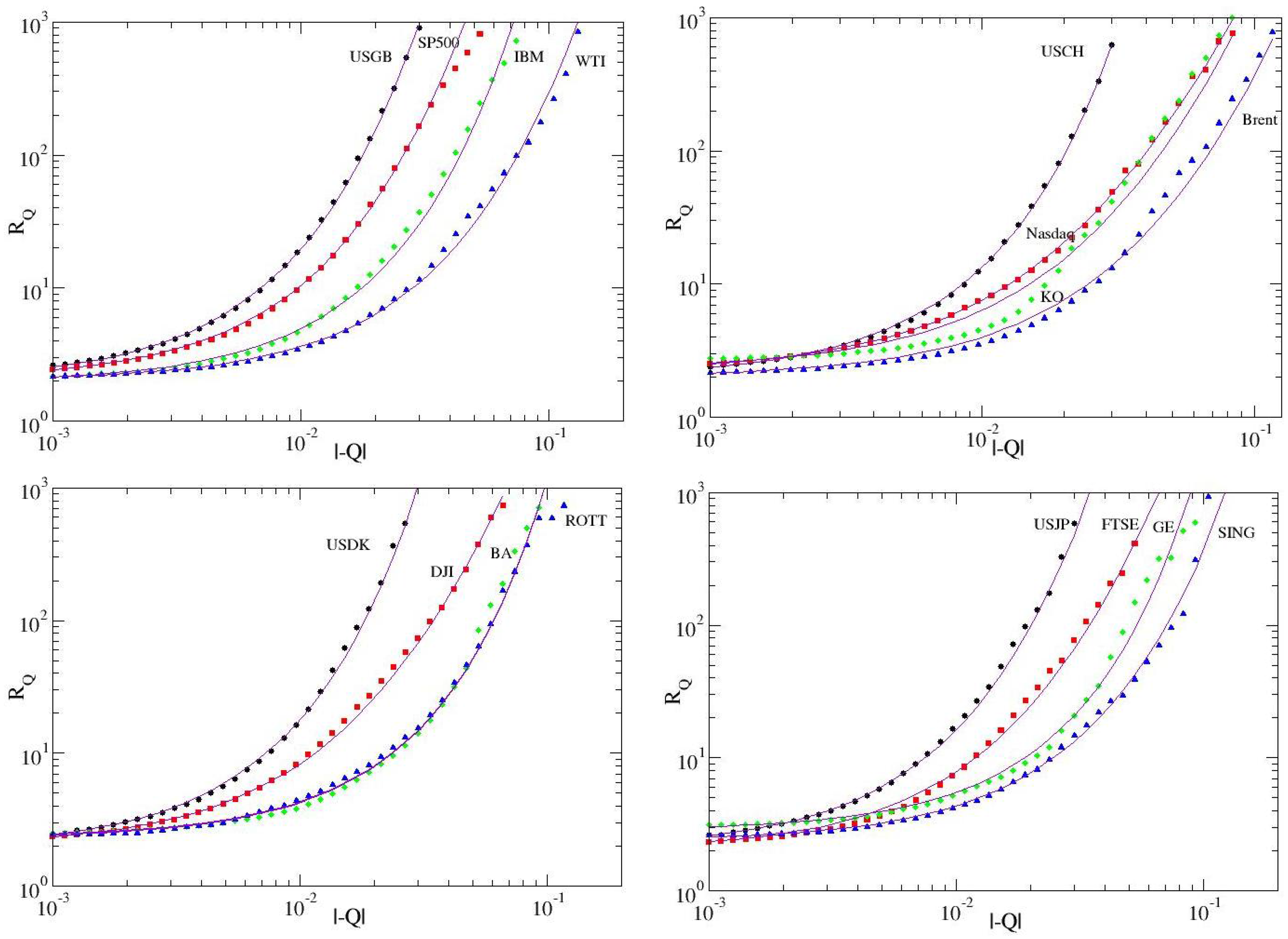
Figure 8.
The mean inter-occurrence time versus the absolute value of the loss threshold −Q: versus the representation of the same data of Figure 7. The continuous curve is a fitting with . From [107].

Figure 9.
(a) The distribution function of the inter-occurrence times for the relative daily price returns of IBM in the period 1962–2010. The data points belong to = 2, 5, 10, 30 and 70 (in units of days), from bottom to top. The full lines show the fitted q-exponentials for typical values of . (b) The dependence of the parameters (squares, lower curve) and (circles, upper curve) on in the -exponential. (c) Confirmation that, for , the distribution function is a simple exponential (i.e., ). The straight line is proportional to . From [106].
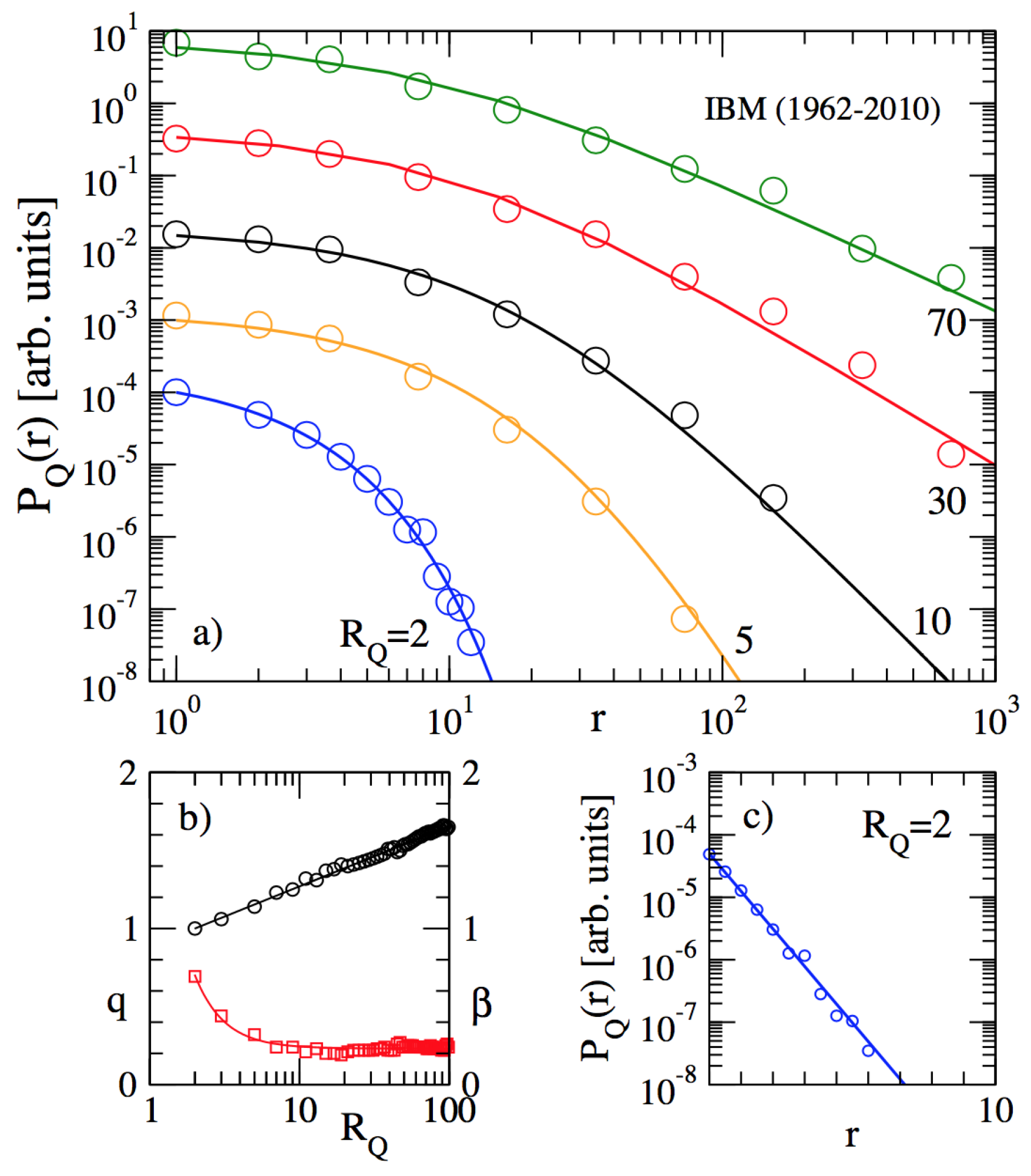
Figure 10.
The distribution function of the inter-occurrence times (as in Figure 9a) for the relative daily price returns of 16 examples of financial data, taken from different asset classes (stocks, indices, currencies, commodities). The assets are: (i) the stocks of IBM, Boeing (BA), General Electric (GE), Coca-Cola (KO); (ii) the indices Dow Jones (DJI), Financial Times Stock Exchange 100 (FTSE), NASDAQ, S&P 500; (iii) the commodities Brent Crude Oil, West Texas Intermediate (WTI), Amsterdam-Rotterdam-Antwerp gasoline (ARA), Singapore gasoline (SING); and (iv) the exchange rates of the following currencies versus the U.S. Dollar: Danish Crone (DKK), British Pound (GBP), Yen, Swiss Francs (SWF). The full lines show the fitted q-exponentials, which are the same as in Figure 9a. From [106].
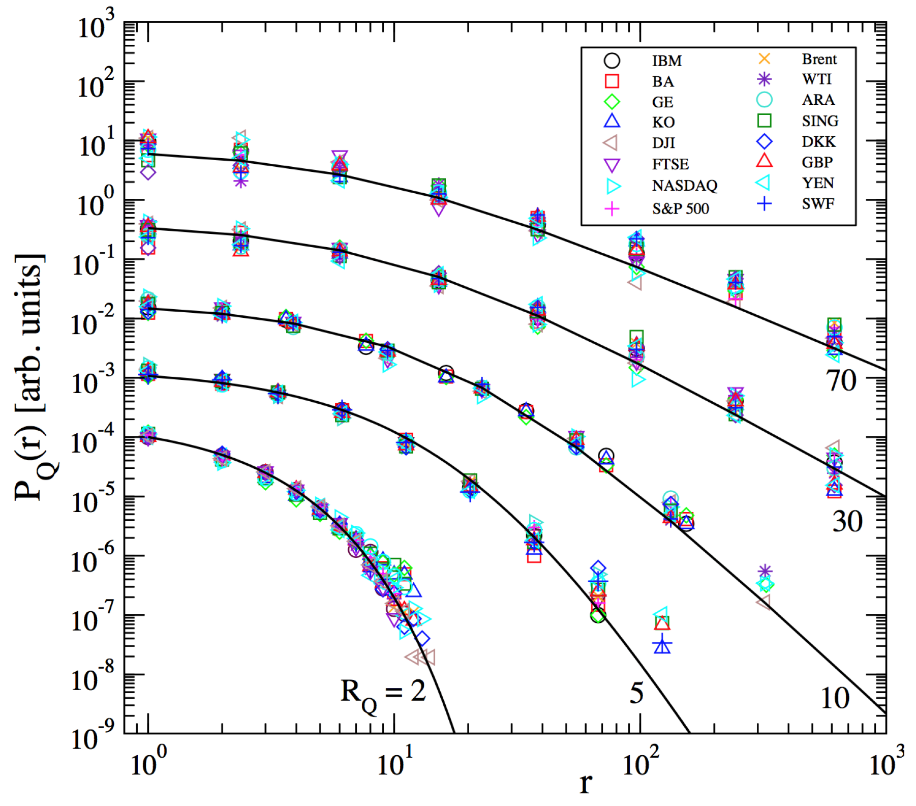
Figure 11.
Universal risk function from Equation (23) for the inter-occurrence time = 100 and for the intervals = 1, 5, 20, 100 days (from bottom to top). From [106].
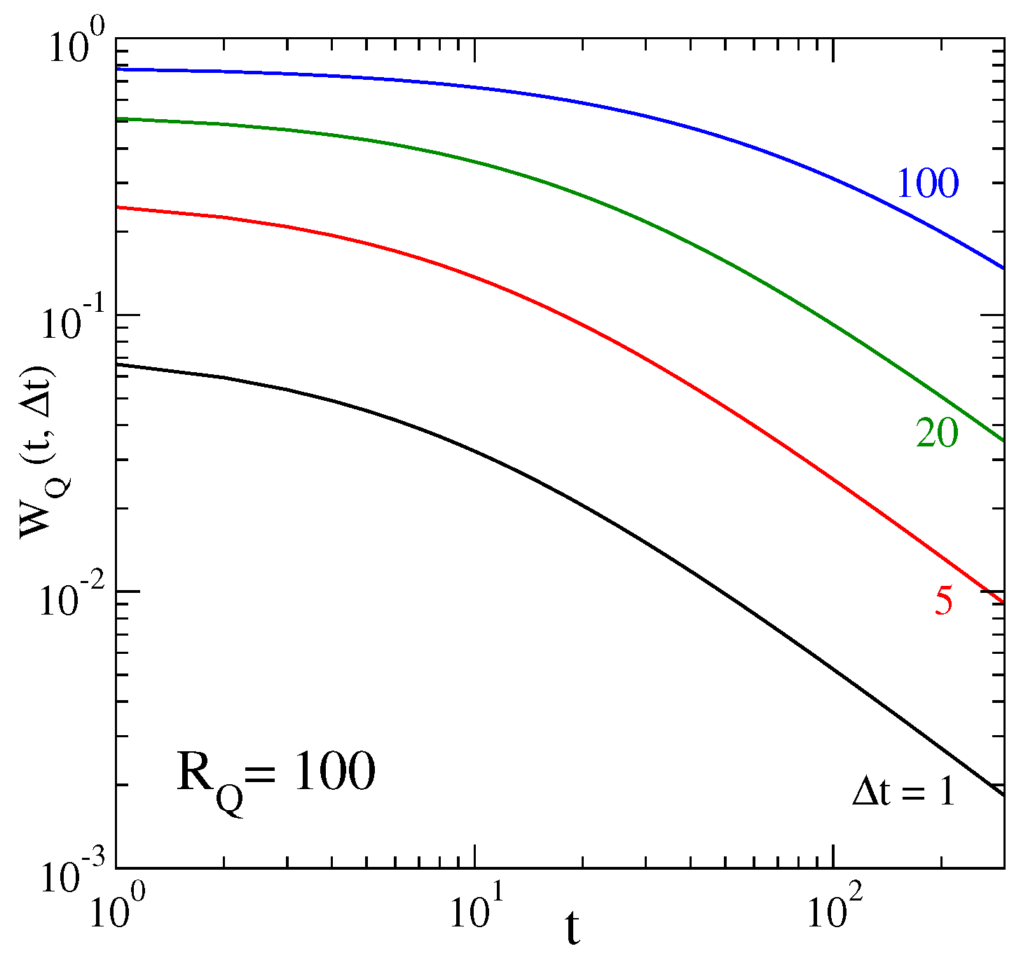
Figure 12.
Binned inverse cumulative distribution of the county, (U.S.) and (Brazil, Germany and U.K.), where denotes the Personal Income and denotes the Gross Domestic Product of countries. Three distributions are displayed for comparison: (i) q-Gaussian (with ) (dot-dashed); (ii) ()-Gaussian (solid) and (iii) log-normal (dashed lines). (a,b) present insets with a linear-linear scale, to make more evident the quality of the fitting at the low region (in (c,d), the ()-Gaussian and the log-normal curves are superposed and, so, are visually indistinguishable). The positions of the knees are indicated. The ankle is particularly pronounced in (c), though it is also present in the other cases. From [105], where further details are available.

Figure 13.
Evolution of parameter q for the U.S. (squares), Brazil (circles), the U.K. (up triangles) and Germany (down triangles). The parameters (for each country) are constant for all years: = 2.1, = 1.7, = 1.5, = 1.4. Lines are only guides to the eyes. As we verify, in some cases, the index q remains invariant along time, whereas in others, it evolves; the functional forms remain however the same as indicated in Figure 12. From [105].
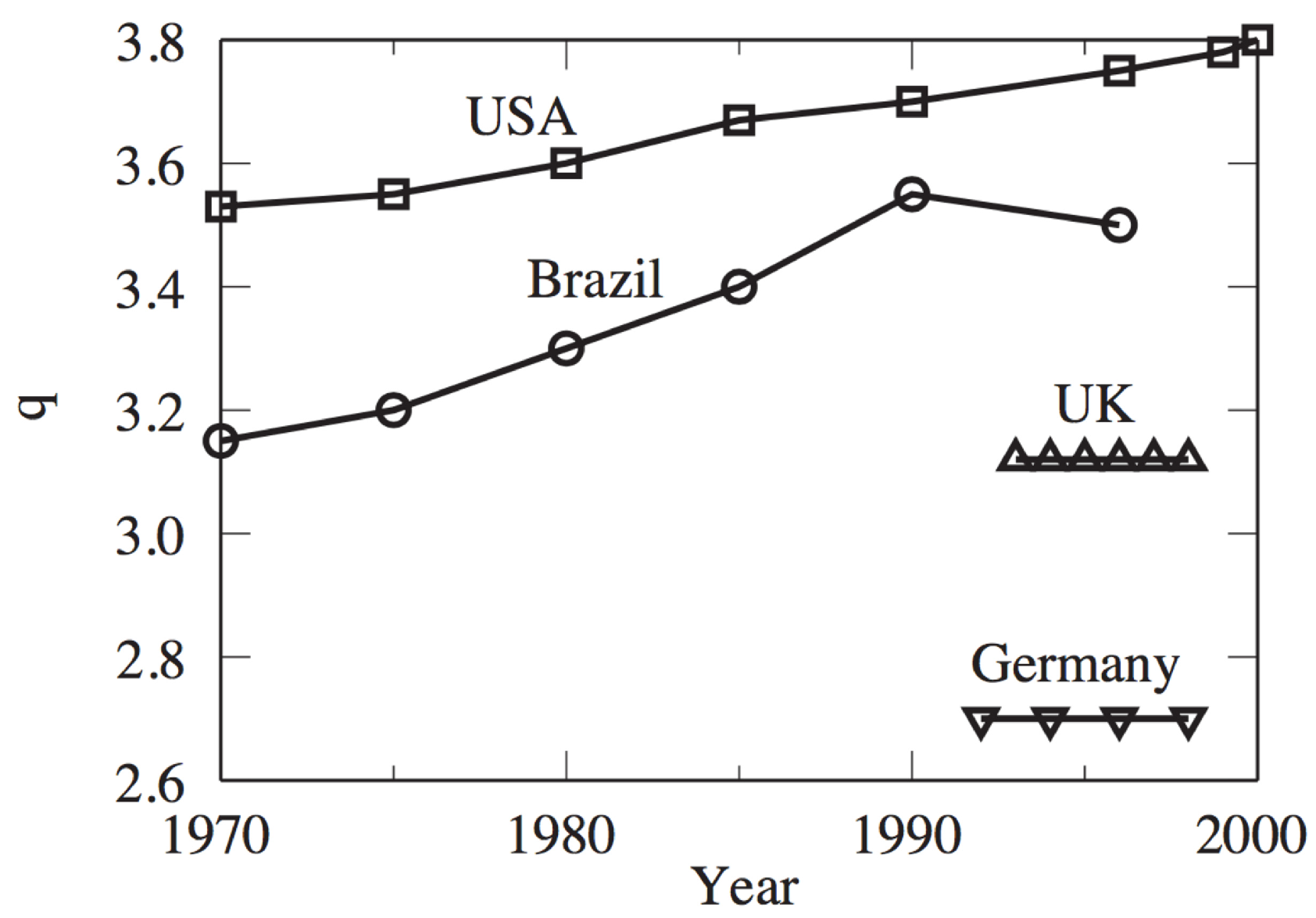
Figure 14.
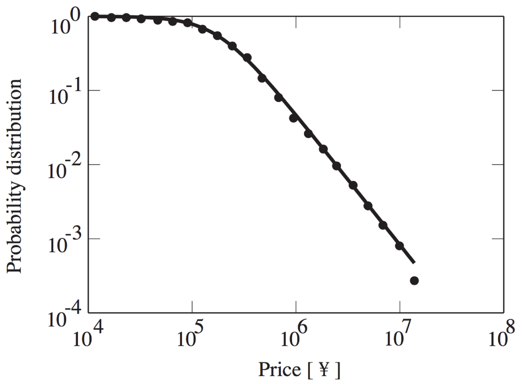
Inverse cumulative probability distribution of Japanese land prices for the year 1998. The solid curve is a q-Gaussian with , which corresponds to the slope , and 188,982 Yen. From [105], where further details are available.
Figure 14.
Inverse cumulative probability distribution of Japanese land prices for the year 1998. The solid curve is a q-Gaussian with , which corresponds to the slope , and 188,982 Yen. From [105], where further details are available.

© 2017 by the author. Licensee MDPI, Basel, Switzerland. This article is an open access article distributed under the terms and conditions of the Creative Commons Attribution (CC BY) license (http://creativecommons.org/licenses/by/4.0/).
Share and Cite
MDPI and ACS Style
Tsallis, C. Economics and Finance: q-Statistical Stylized Features Galore. Entropy 2017, 19, 457. https://doi.org/10.3390/e19090457
AMA Style
Tsallis C. Economics and Finance: q-Statistical Stylized Features Galore. Entropy. 2017; 19(9):457. https://doi.org/10.3390/e19090457
Chicago/Turabian StyleTsallis, Constantino. 2017. "Economics and Finance: q-Statistical Stylized Features Galore" Entropy 19, no. 9: 457. https://doi.org/10.3390/e19090457
Note that from the first issue of 2016, this journal uses article numbers instead of page numbers. See further details here.