Thermodynamics of Small Magnetic Particles
by
Eugenio E. Vogel
1,2,*, 
Patricio Vargas
2,3, 
Gonzalo Saravia
1,
Julio Valdes
1,
Antonio Jose Ramirez-Pastor
4 and
Paulo M. Centres
4 1
Department of Physics, Universidad de La Frontera, Francisco Salazar 01145, Temuco, Chile
2
Center for the Development of Nanoscience and Nanotechnology, 9170124 Santiago, Chile
3
Department of Physics, Universidad Técnica Federico Santa María, Avenida España 1680, Valparaíso, Chile
4
Departamento de Física, Instituto de Física Aplicada, Universidad Nacional de San Luis-CONICET, Ejército de Los Andes 950, San Luis D5700BWS, Argentina
*
Author to whom correspondence should be addressed.
Entropy 2017, 19(9), 499; https://doi.org/10.3390/e19090499
Submission received: 2 August 2017
/
Revised: 1 September 2017
/
Accepted: 13 September 2017
/
Published: 15 September 2017
(This article belongs to the Special Issue Thermodynamics and Statistical Mechanics of Small Systems)
Abstract
:In the present paper, we discuss the interpretation of some of the results of the thermodynamics in the case of very small systems. Most of the usual statistical physics is done for systems with a huge number of elements in what is called the thermodynamic limit, but not all of the approximations done for those conditions can be extended to all properties in the case of objects with less than a thousand elements. The starting point is the Ising model in two dimensions (2D) where an analytic solution exits, which allows validating the numerical techniques used in the present article. From there on, we introduce several variations bearing in mind the small systems such as the nanoscopic or even subnanoscopic particles, which are nowadays produced for several applications. Magnetization is the main property investigated aimed for two singular possible devices. The size of the systems (number of magnetic sites) is decreased so as to appreciate the departure from the results valid in the thermodynamic limit; periodic boundary conditions are eliminated to approach the reality of small particles; 1D, 2D and 3D systems are examined to appreciate the differences established by dimensionality is this small world; upon diluting the lattices, the effect of coordination number (bonding) is also explored; since the 2D Ising model is equivalent to the clock model with degrees of freedom, we combine previous results with the supplementary degrees of freedom coming from the variation of q up to . Most of the previous results are numeric; however, for the case of a very small system, we obtain the exact partition function to compare with the conclusions coming from our numerical results. Conclusions can be summarized in the following way: the laws of thermodynamics remain the same, but the interpretation of the results, averages and numerical treatments need special care for systems with less than about a thousand constituents, and this might need to be adapted for different properties or devices.
1. Introduction
Recent developments in experimental techniques and refinements of synthesis methods allow for direct measurements of very small systems [1,2,3,4,5,6]. Examples of such systems include magnetic domains in ferromagnets, which are typically smaller than 300 nm, quantum dots and solid-like clusters that are important in the relaxation of glassy systems and whose dimensions are a few nanometers. Due to the small size of such systems and the high surface/volume ratio, the usual thermodynamic properties of macroscopic systems do not apply in the usual sense, and the analysis of fundamental principles of statistical thermodynamics needs to be reconsidered [7,8,9,10]. Phase transitions, specific heat, thermal conductivity, magnetization and other phenomena need careful examination of the corresponding thermodynamic variables used to characterize them. Ergodicity, fluctuations and error bars are among the aspects that are greatly affected by the small size of the systems.
The increasing interest in the theory of small systems is not limited to physics, but also extends to biological and chemical systems, such as clusters [11,12], thin films [13] and biological molecular machines with sizes under 100 nm [14]. This broad picture calls attention to the extension of the mathematical treatments valid in the (usually called) thermodynamic limit (TL) to systems formed by a small number of elements.
In 1962, Hill [15,16] developed a formalism for describing the thermodynamics of small systems, where thermodynamic properties such as enthalpy and Gibbs energy are no longer extensive. The pioneer work of Hill established the fundamental laws that govern finite-size effects in thermodynamics. Later, Hill and Chamberlin [17,18,19,20] introduced the term nanothermodynamics to denote the study of systems far away from the TL. Despite these results, there are still many open questions regarding the thermodynamic behavior and possible applications of very small systems.
Magnetic nanoparticles [21,22] are also examples of small systems whose properties are influenced by finite size effects. The competition between core and surface effects determines the state of the particle, which can go from a paramagnetic state to a ferromagnetic state. The temperature characterizing this transition is the well-known Curie temperature () in the TL. Experimental studies for different materials show that the in nanoparticles is not a unique property of the material (as in the bulk), since it is strongly size dependent and decreases as the characteristic dimension of the particle, (where V is the volume of the particle), is reduced [23,24,25].
In a recent work [26], it has been shown that for tiny systems, not only surface sites are special, but also some inner sites might not be equivalent to each other. This fact can have important consequences on the thermodynamic properties of small nanoparticles (up to sizes of the order of ≈10 nm). In the magnetic systems described below, this effect mainly introduces dispersion in the exchange coupling constants, which in turn may affect the values of the thermodynamical parameters. These considerations tend to lose importance as the nanoparticle size increases. Moreover, they do not affect the overall underlying physics, but impose limitations in the interpretation of the magnitudes defined in the TL.
In the present paper, we would like to answer the following questions: How stable and reliable are devices built of subnanoscopic magnetic particles? How do the representative properties of these devices depend on the size, dimensionality, coordination and internal degrees of freedom among other variables? We will consider two examples offered by very small magnetic particles responding to temperature changes; such particles could be components of devices.
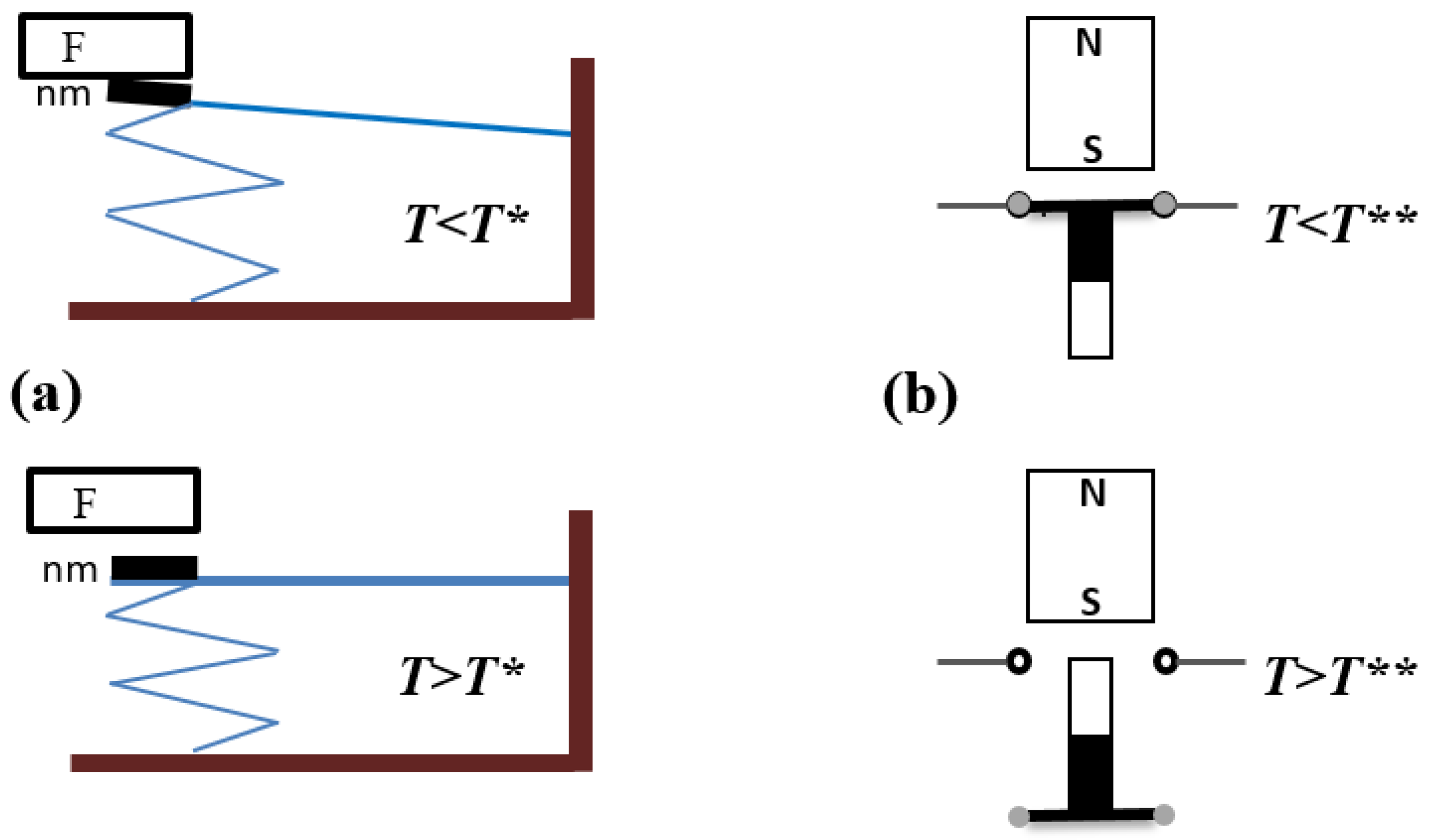
Let us first consider the magnetic switch shown in Figure 1a where a tiny nanomagnet (nm) sticks to a ferromagnetic material (F) under a sensitive temperature (a way to avoid calling it the critical temperature). To overcome the difficulties of defining temperature for very small isolated systems we will assume that the devices and everything that is connected to them are immersed in a thermal bath at temperature T. Changes in temperature are smooth and slow, so there is time to equilibrate. As temperature raises, nm can decrease its magnetization under a critical value, which will weaken the attraction to F; then an elastic restoring force (like the spring in the figure) brings nm to its natural position away from F. This magnetic switch could activate an alarm that goes off over a prefixed temperature, which ideally is precisely . Let us assume that for this system, mechanical relaxation times are longer than electronic ones; then, such a device is not sensitive to magnetization reversals, so it is basically controlled by the absolute value of the magnetization, namely ||.
Figure 1b presents a tiny rod-like nanomagnet, which can rotate about its center on the plane of the figure. A stronger fixed magnet (NS) with high orientates the tiny magnet. When the temperature goes over a sensitive temperature , a magnetization reversal happens in the small magnet. Such polarity reversion triggers a rotation of the small particle disconnecting the terminals that are connected when the conducting element attached to the “black” part of the particle closes the circuit. This device is strongly dependent on the polarity of the nanoparticle, namely on the sign of . Magnetization reversals are usually quite fast as compared to most mechanical processes in materials. Some orders of magnitude for the switching time (defined as the time in which the magnetization reverses polarity) have been proposed at about 200 ps for small Co systems [27]. The switching time could be larger depending on the system size, temperature and magnetic anisotropies, but a few tenths of ns have been reported for other small systems in the absence of an external magnetic field [28].
We shall come back to these examples later on since this is the kind of system we have in mind, rather than statistical averages over different samples or instances. At this stage, we point to the gross picture, namely the tendency of properties, and not to material-related or geometrical features controlling a particular device. To focus the discussion, we turn our attention to two general and well-known models whose properties can be reexamined in this new scenario. We refer to the Ising model and to the clock model (related to the better-known Potts model).
The Ising model plays a central role in the study of phase transitions in magnetic systems (transitions from paramagnet to ferromagnet, order-disorder transitions, etc.) [29,30,31,32,33,34,35,36,37]. Ising [38] gave an exact solution to the one-dimensional lattice problem in 1925. All other cases are expressed in terms of series solution [39,40], except for the special case of two-dimensional lattices in zero external field, which was exactly solved by Onsager [41] in 1944. Close approximate solutions in dimensions higher than one can be obtained, and the two most important of these are the mean-field approach [42] and the quasi-chemical approximation [42,43].
In the last few years, the Ising model has been adopted as a prototype for studying the magnetic properties of systems far away from the TL [44,45,46]. In [44], Velásquez et al. studied the magnetic properties and pseudocritical behavior of ferromagnetic pure and metallic nanoparticles in the presence of atomic disorder, dilution and competing interactions. Using variational and Monte Carlo methods, the authors reported the particle size dependence of the ordering temperature for pure and random diluted particles.
Bertoldi et al. [45] solved analytically the Ising model for small clusters in the microcanonical formalism, using the mean-field theory and considering the presence of surfaces. In agreement with the work of Velásquez et al. [44], the authors found that the critical temperature decreases proportionally to the inverse of the radius of the cluster. Recently [46], the Ising model on a simple-cubic lattice was used to analyze the main concepts of nanothermodynamics applied to Monte Carlo simulations.
Finally, we increase the internal degrees of freedom at each site upon generalizing the Ising model to the discretized XY model in what is called the clock model which is a well-known example of the famous Berezinskii–Kosterlitz–Thouless (BKT) transition [47,48]. In this way, we will be able to appreciate what is the role of the increase of the configuration space due to the characteristics of the constituents of small systems and not only the fact that they interact among themselves.
This paper is organized as follows: In Section 2, we present the system and the methodology based both on theoretical formulations and on computer simulations. In Section 3, we present the results stressing those points where the analysis concerning the TL is not applicable for very small particles; the discussion and relations among results are done along with the presentation of the results given by plots and particular numerical values. In Section 4, we list and comment on the main conclusions.
2. Model and Methods
2.1. General Definitions
Let us begin by considering the Ising model on a square lattice of dimensions , where local magnetic moment or “spin” at site i can point either along the positive () or negative direction () of a given axis. The isotropic Hamiltonian for such a system can be written as:
where J is the exchange interaction to nearest neighbors; the sum extends to all pairs through the lattice, which is indicated by the symbol under the summation symbol. The magnetization of the system at any temperature T and time t is simply obtained by just adding the spins in an algebraic manner, namely,
where we have normalized it over the number of sites N, which is equivalent to normalizing it with respect to the saturation magnetization.
Large macroscopic systems are modeled by making use of periodic boundary conditions (PBC) where surface states are ignored; in this approximation, Lars Onsager [41] found an analytic solution for the magnetization of the system in 2 dimensions (2D):
where is the Boltzmann constant, which we can take as 1.0 from now on (this is equivalent to measuring energy and J in T units). The critical temperature can be readily obtained at the point where the magnetization vanishes:
Then, the exact numeric solution for this problem for PBC can be easily evaluated, yielding:
where J has been omitted, as will be done from now on.
The reason to have chosen the 2D Ising model to begin with is precisely this result, namely the existence of an analytic solution for the transition temperature in the TL. We can use it as a reference point to compare with other results and simulations where different conditions will be varied.
2.2. Exact Theoretical Approach for a Small System
Next, we consider a very small Ising square lattice, , where we can calculate everything exactly. The partition function can be expressed as:
where the coefficients give all of the possible spin configurations compatible with energy according to the Ising Hamiltonian; is the number of energy levels.
We can write the exact partition functions and for PBC and free boundary conditions (FBC), respectively:
where coefficients and are to be obtained from Table 1 and Table 2, respectively. These tables list the corresponding degeneracies (PBC) and (FBC) for the set of states sharing energy given by Equation (1) and magnetization :
which runs between and at intervals of 2, as shown by the second row in the tables. The coefficients in the expansions given by Equations (7) and (8) can be obtained as:
where we take into consideration the symmetry in Table 1 and Table 2, namely and with , and
It should be noticed that Table 1 and Table 2 give only those configurations with nil or positive magnetization. However, the Hamiltonian above is symmetric under the simultaneous reversion of all spins, so both tables should be continued to the left to include the states with negative magnetization.
2.3. Numerical Simulations
In addition to some theoretical calculations, most of the work will deal with numerical calculations based on Monte Carlo (MC) simulations. A square lattice is chosen; PBC or FBC are imposed; a site is randomly visited; and the energy cost of flipping the corresponding spin is calculated: if the energy is lowered, the change of orientation is accepted; otherwise, only when , the spin flip is accepted, where r is a freshly-generated random number in the range [0,1]. This is the usual Metropolis algorithm. A Monte Carlo step (MCS) is reached after spin-flip attempts. One of the main goals here is to report the sensitive temperatures ( or analogues to critical temperatures in the TL) for different systems.
The energy is computed according to the Hamiltonian given by Equation (1). The instantaneous magnetization at time t and temperature T is obtained from Equation (2).
For each temperature, MCSs are performed: the first MCS is used to equilibrate at a fixed temperature T, while the second MCS is used to measure the magnetization every 20 MCSs, reaching a total of 50,000 measurements. Unless specified in a different way in the rest of the paper; this value gives stable results and leads to coincidence with the analytic expressions obtained as described above.
2.4. The Clock Model
This is the discrete version of the famous 2D XY model, which is probably the most extensively studied example showing the Berezinskii–Kosterlitz–Thouless (BKT) transition [47,48]. It is often used as a reference of its peculiar critical behavior at the transition point and universal features [49,50,51,52,53]. Instead of the exclusion of an explicit continuous symmetry essential for the BKT transition, it can also emerge from a system without explicit continuous symmetry. The q-state clock model is the discrete version of the XY model, with discrete symmetry. The Hamiltonian of the clock model can be written as:
where is the ferromagnetic coupling connecting pairs of nearest neighbors i and j; the discrete angle between the spin orientations is given by , for . While the exact XY model is recovered only in the limit of infinite q, it has been found that the BKT characters appear in the clock models when [54,55,56,57]. The nature of the phase transitions in the general clock model has been widely studied with different theoretical and numerical approaches, which however have given mixed results on the characterization of transitions at the lower bound of q (for instance, see the summary of the related debates in [58]).
In spite of all that, in this work, we want to use this model as a generalization of the Ising model presented above allowing for the increase in the number of internal states at each site. All of this is always aimed at the behavior of small systems. We will focus on a square lattice 8 × 8 with FBC, with the clock model ranging from (Ising model) to (one discrete version of the 2D finite XY model).
3. Results and Discussion
Let us begin by considering the theoretical approach for the Ising lattice with introduced in the previous section. The magnetization per site can be calculated as:
and:
both of which give a nil result for any T since negative and positive contributions to the magnetization cancel out as they are weighted with the same probability due to the symmetry properties of Table 1 and Table 2.
In macroscopic systems, ergodicity is spontaneously broken favoring any of the two halves of the configuration space. As we will see below, this is not always true for very small systems, but let us start from the ergodicity breaking approach so widely invoked to approach the TL. This can be achieved by either considering only the positive magnetization contributions of Table 1 and Table 2 plus half of the coefficients for the column of the corresponding table. Equivalently, we can force ergodicity breaking by considering all of the contributions to the magnetization, but using their absolute value, namely,
and:
where e refers to the forced ergodicity breaking.
We invoke now the numeric simulations defined in the previous section to calculate the magnetization for the same system. Here, the same trick is done to break ergodicity, namely it is always || (obtained from Equation (2)) that is considered as the contribution to magnetization from every configuration visited. In this way, ergodicity breaking is forced to occur in any circumstance. We will call (PBC) and (FBC) the magnetizations obtained via numeric simulations for a temperature T and at an instant t.
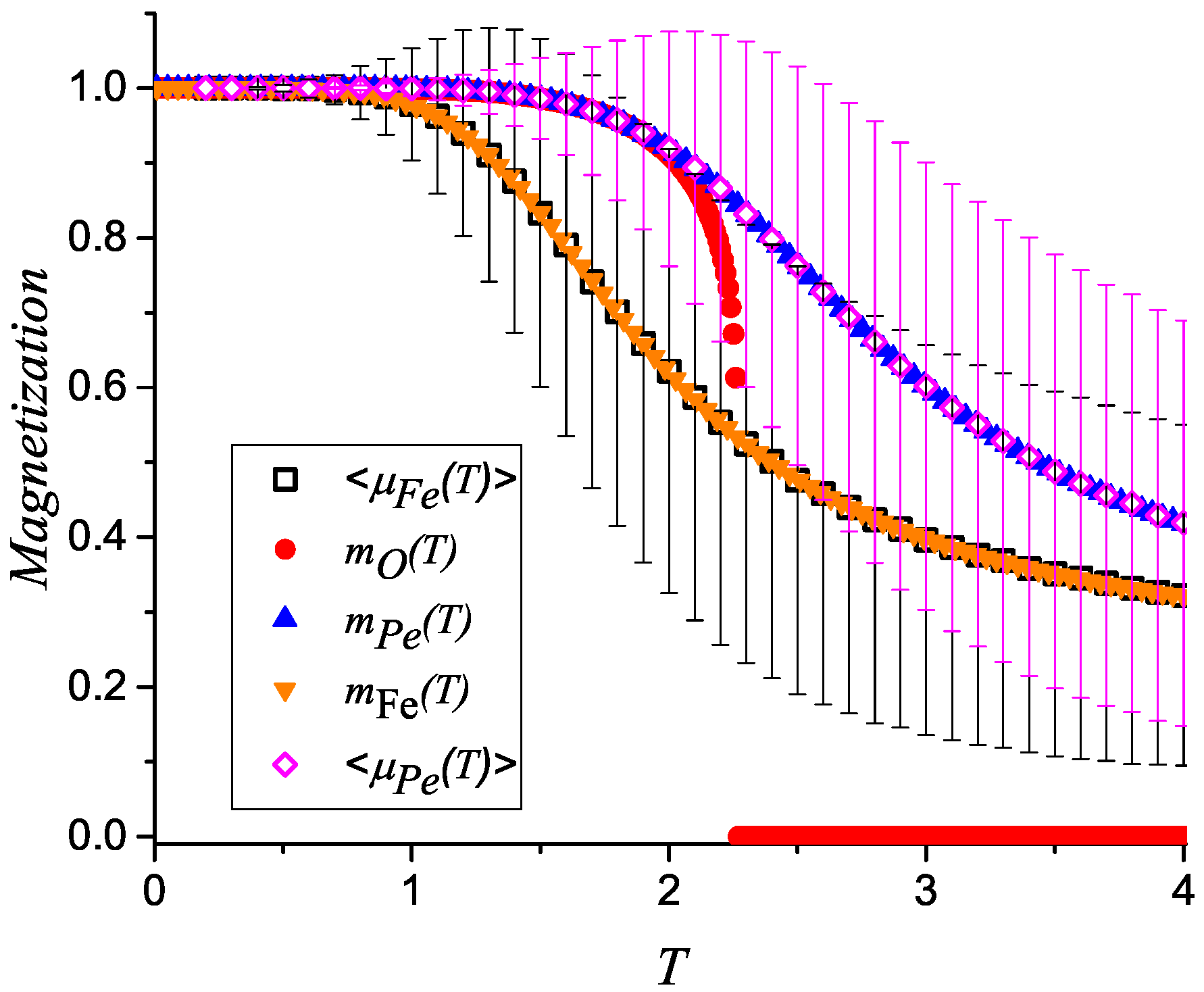
We compare now previous approaches. Results from Equations (16) and (17) are shown by up and down solid triangles respectively in Figure 2. The results for the numeric simulations for PBC and FBC are shown here by empty diamonds and empty squares respectively. The values for and reported in Figure 2 correspond to positive averages over 50,000 measurements. The corresponding distribution of values allows us to report the error bars for each temperature.
For comparison and discussion, the Onsager solution is also added to this figure by means of solid circles.
Figure 2 deserves a careful analysis and discussion. The excellent agreement between theory and numeric simulation is very impressive. However, this should not be very surprising since the Metropolis algorithm is based on the same probability laws that appear in the partition function, hence, in the magnetization as well; both approaches consider ergodicity breaking, as already pointed out. The agreement is stressed in the sense that the computer algorithms used here are very reliable, and the equilibration times are enough. It can be noticed that both the theoretical and numeric results for PBC coincide with the Onsager solution up to almost . From there on, both treatments overestimate the magnetization values partly due to a small size effect, but also due to the forced ergodicity breaking, which is assumed in these calculations. We will come back to this point below.
Let us now pay attention to the different results obtained for FBC as compared to PBC regardless of the method employed in the calculation. It is PBC that can be used to compare with the results valid in the TL, which are illustrated in Figure 2, by the Onsager solution yielding . As can be seen, the theoretical results and magnetic simulations using PBC both agree with the Onsager solution up to approximately; from there on, both solutions remain at high values, decreasing smoothly without an indication for a sharp phase transition. In the case of very small particles, PBC are unthinkable, since in this limit, surface states become very important. This is an indication that FBC should be used to model the properties of very small particles.
The light and smooth decrease in magnetization due to surface effects will determine that the nanomagnets involved in the simple systems of Figure 1 will have different responses as those made of the same basic material, but operating in the bulk sizes, namely in the TL. The sensitive temperatures and for which these devices will activate still depend on other features to be examined below, but this is a first result showing that properties characterized in the bulk need to be reexamined for very tiny particles.
Actually, we can define the corresponding sensitive temperature simply as the temperature for which or (with any subscripts) takes the value 0.5. This working definition is consistent with the TL, where a square step magnetization curve is expected at (equivalent to our sensitive temperature), jumping from magnetization 1.0 to 0.0. Then, the sensitive temperatures can be read from Figure 2 as 2.4 and 3.4 for FBC and PBC, respectively. Both values are larger than the macroscopic expected result, which requires further discussion.
What is the real meaning of the average values we have just reported? Let us revisit the FBC data and do a different exercise: let us plot the instantaneous value of the magnetization (no ergodicity breaking here) after the instants of measurement (last measured value for each temperature after total MCSs). This is plotted by solid squares (black) in Figure 3 using the same data already available from FBC on the lattice. These results allow for just one interpretation: at least at (or eventually at even lower T values), a magnetization reversal occurred, and ergodicity breaking is no longer valid. Therefore, the previous approach intended for the TL has to be reconsidered to analyze the results obtained in the small world. This is an indication that the ergodicity breaking assumption is valid only for systems over a minimum size and appropriate for the property under investigation.
All of the previous procedures are usual for TL analysis. However, the magnetic switches presented in the Introduction will respond instantaneously and without having the chance of performing derivatives, averages or even more sophisticated mathematical analyses, like the crossing of Binder cumulants [59] or the crossing of autocorrelation functions [60], to decide which is the appropriate value for the sensitive temperature. In these examples and in all nanosized devices, a careful analysis of the thermodynamics of the object in terms of the desired property should be appropriately done.
In the case of the magnetic switch illustrated by Figure 1a, the nanomagnet (nm) will stick to the ferromagnetic material (F) regardless of its polarity. This would be the case of systems whose magnetization reversals are much faster than any mechanical process (like elastic forces) usually involving atomic masses. Therefore, such a device would be insensitive to magnetization reversals and will respond effectively to the magnitude of the magnetization of the nm switching off the circuit at a certain sensitive temperature .
On the other hand, in the case of the magnetic switch illustrated by Figure 1b, the magnetic nanorod will always point with its north pole to the fixed magnet on top, which coincides with the black portion of the rod in the upper part of this figure at low T values. As temperature rises, a magnetization reversal is possible in the softer magnetic material in the nanorod; the north pole is now on the white part of the rod, and the nanomagnet will rotate with respect to its fixed center. Therefore, this device is sensitive to the polarity of the nanomagnet and will disconnect the circuit at a certain sensitive temperature .
Even if the nanomagnets in both switches are made of the same material, and will be different in general because they originate from different properties: the former is governed by the value of the absolute magnetization, and the latter responds to the reversal process depending on the instantaneous sign of the magnetization. As we will show below, they are different indeed, and for the systems to be studied, .
Figure 3 also yields the average of the actual instantaneous magnetization values obtained for FBC over the 50,000 instants, namely,
These results are reported by means of empty circles (red) with the corresponding error bars. If we look at these data, we should estimate .
By enforcing ergodicity breaking in Figure 2 and Figure 4, we are biasing the data in several senses: magnetization reversals are inhibited as if there is an infinite anisotropy; the instability of the systems is ignored; the curve is artificially smoothed; the average value of the magnetization is always positive; and it does not converge to 0.0 as . This last result is usually confused with the tails of the magnetization curves (and other order parameters) for due to finite size effects.
From the previous discussion, it is clear that a unique definition for a Curie temperature in the nanoworld faces huge difficulties. At least the usual definition of a Curie temperature, where all magnetic properties change at one precise temperature, is not longer sustainable. Actually, in the TL, there would not be a difference between the two switches illustrated in Figure 1. However, we have just shown that for a magnetic systems of just very few interacting elements, different properties may have different sensitive temperatures.
The general message here is that when dealing with small particles, instantaneous responses may have a great importance and could determine completely the performance of the device. The details of this behavior will depend on the properties involved, geometry and other characteristics.
In any case, what is quite clear is that is not the only property governing the response of the device at very small sizes. The large error bars in Figure 2 and Figure 4 indicate that instantaneous measurements of magnetization can be erratic and at times could disconnect the device at unexpected temperatures under the desired one. As sizes get larger, error bars progressively decrease, and becomes the right parameter to design devices as those shown in Figure 1.
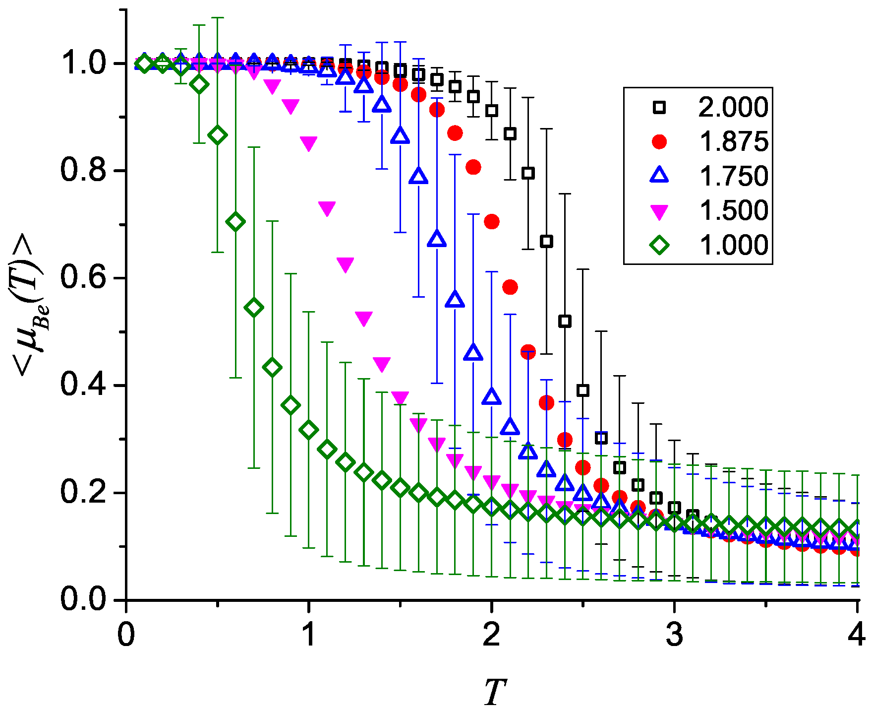
Another important result shown by Figure 2 is the huge size of the error bars, which are likely associated with the small size of our system. To test this hypothesis, we will do numerical simulations similar to those of Figure 2 using both PBC and FBC for . Results (along with others to be defined immediately below) are presented in Figure 4 by empty squares and solid circles, respectively. In fact, error bars are now smaller; has moved to lower values; the slope in the descent is more vertical (approaching the square step shape expected at the TL); and the remnant absolute magnetization towards high temperatures has decreased. Therefore, it is clear that we are moving in the direction where these simulations designed for the TL are effective.
We can make use of this opportunity to discuss another important consideration for small particle behavior: coordination number (or bonding, to put it in a more general context). Let us define effective coordination number as the ratio of the number of bonds B (nearest neighbors in our case) over the number of the N individuals (spins) interconnected by these B bonds. For any square lattice with PBC, and ; the upper index (2) refers to 2D. In the case of FBC, we have ; , so:
which for , yields , as illustrated in the inset of Figure 4. It is clear that in the TL, , but for small particles, the difference might matter.
The effective coordination number defined above can be diminished upon diluting the original lattice. This can be achieved by human decoration on the original lattice (just removing atoms in a prescribed way) or could be due to some natural process that takes away magnetic atoms of our 2D sample (corrosion for instance). For simplicity, we will have the first alternative in mind, but the results for the second one would only add randomness to what we will discuss next.
Let us go back to the ferromagnetic lattice , and we will progressively dilute it upon removing four square sectors each time in the way shown in Figure 5 for the case . To be more specific, the lattice is divided into four sectors , and the extraction of the sites is done from the lower right corner of each sector. For the example under consideration, and , so . Then, we remove four sectors with and, finally, four sectors with , obtaining and , respectively. In all of these cases, FBC are imposed. The last case is quite interesting because it is equivalent to the linear chain used by Ernest Ising in his original (and only) paper [38], for which the expected is 0.0, namely no phase transition for finite temperatures.
Results for are given in Figure 4, where the values of are given in the inset. Error bars were also calculated for all values, but they are shown for 2.000, 1.750 and 1.000 only for the simplicity of the figure. Direct comparison shows that error bars for the lattice 16 × 16 are less pronounced than the corresponding ones for the lattice 4 × 4.
The main result of Figure 4 is to show the way decreases as the effective coordination number decreases. This is even more so if ergodicity breaking is imposed, an effect that we will discuss again below.
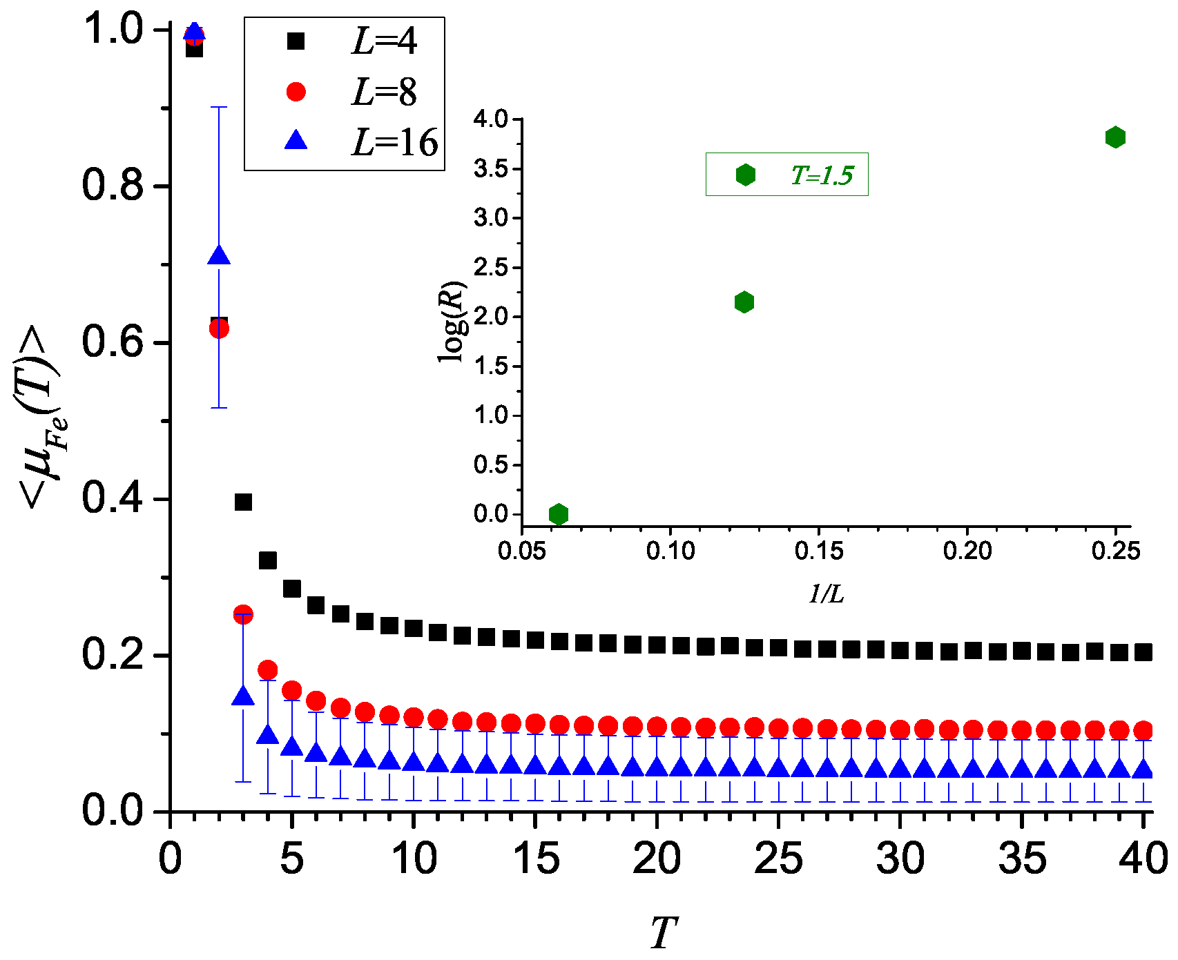
Let us stress another shortcoming of the forced ergodicity breaking method mentioned before, namely the fact that remains positive at high temperatures. In Figure 2, the last point of the simulation corresponds to with error bars of about for FBC. For this lattice, we can actually make use of Equation (17) to obtain the exact value in the high T limit: , which indicates that temperature has to be increased in the numeric simulations to attain a better comparison. We can follow this tendency simulating higher temperatures including larger lattices. Thus, Figure 6 shows results for 4, 8 and 16, where the positive asymptotic behavior is clearly shown; the values for are 0.204, 0.104 and 0.052, respectively. The first result is approaching the already quoted theoretical result 0.196. The set of values indicates that this sort of imposed remnant magnetization tends to be negligible for large lattices in the TL. A different way to put this is that magnetization reversals decrease as L increases, which makes the imposed ergodicity breaking coincide with the real ergodicity breaking. This tendency is shown in the inset of Figure 6 where in the logarithmic scale, we plot the number of magnetization reversals during the 50,000 measurements as a function of for . For higher temperatures, reversals are easier, but the amplitudes are lower; for lower temperatures, reversals are harder, but the amplitudes are higher (which makes the absolute value of stay close to unity). When ergodicity breaking is imposed at low temperatures, magnetization always oscillates between values close to or .
The curve for in Figure 4 deserves a special analysis since it is expected that the magnetization should go down as soon at . However, this figure is for , namely for forced ergodicity breaking, to compare with Figure 2, related to the analytic expressions given by Equations (16) and (17). If we go back to the data for this case, we can study each temperature to find that reversions are occurring at all temperatures. For instance, for in Figure 4; however, if we look at the instantaneous data for the 100 leading intervals of the measuring interval (immediately after equilibration), we find oscillating as given in Figure 7.
For lower temperatures, oscillations are progressively less and less frequent approaching alternations between and only at , where it is necessary to wait a huge amount of time to get the first reversal. In this way, we approach the result for the 1D Ising lattice: no phase transition is possible at a finite temperature.
Let us now investigate the role of the effective coordination number towards the 3D case with PBC (). This is shown in Figure 8, where we begin by a single layer with FBC (); then, we continue the series: two layers with FBC (); three layers with FBC (); four layers with FBC (); four layers , two directions with FBC and one direction with PBC (); four layers , one direction with FBC and two directions with PBC (); four layers , all directions with PBC (). The result is eloquent: moves to higher temperatures as the effective coordination number increases. Moreover, the dimensionality plays also an important role, which can be appreciated when we compare the second case here having , with the already seen case for the PBC lattice (shown in Figure 4). It can be appreciated that for the 3D case, is larger than for the 2D case.
Now, we show results for the q-states clock model simulated on an square lattice. The density of magnetic states increases as q increases; therefore, we expect a q dependence of the sensitive temperature characterizing the transit from an ordered ferromagnetic initial regime to a magnetically-disordered phase.
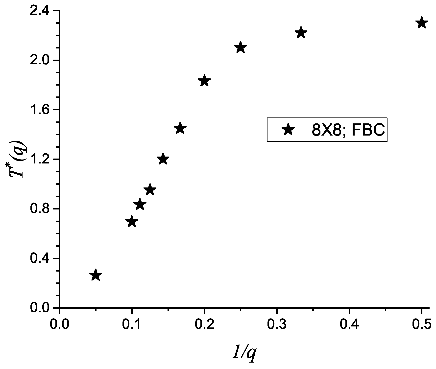
Figure 9 shows the sensitive temperature vs. ranging from to . Here, we follow the same approximation as in Figure 2, namely we force ergodic separation starting always from a ferromagnetic state. is defined as the temperature where the normalized magnetization is , which is a practical way to define the transition to a disordered state. In order to sample with the same density the q-possible states for each spin in the 8 × 8 square lattice (there are states for an 8 × 8 lattice), we increase the number of MCSs as q increases; higher q values need larger numbers of MCS to reach equilibration. Therefore, we use MCSs for the simulations of the q-clock model.
As we see in Figure 9, there is a monotonous decrease of with increasing values of q. Larger values of q mean energy states separated by less energy differences, therefore moving the initial ferromagnetic state to other states with different magnetizations in an easier way: this implies that the disorder for higher q values will be reached at lower temperatures as compared with the starting case (Ising model).
A very striking feature is shown by Figure 9: two regimes are clearly shown: for to , and from to (and possible larger values). In the first regime, decreases with a relatively low slope as a function of , whereas for , the slope of the vs. curve is larger. This change of slope could be associated with different types of transitions that occur for different q values. Namely, there is an order → disorder transition for and a double transition order → quasi-ordered → disordered for as discussed in [58,61].
It is clear from symmetry arguments that as q increases, lower temperatures are sufficient to originate new ferromagnetic states in any of the q directions irrespective of the starting configuration. Therefore, as q tends to infinity, tends to zero. This is known as the Mermin–Wagner theorem [62]. This theorem establishes that there is no magnetic state at any finite temperature () in the XY model. Moreover the formation of vortex-antivortex states is prohibited in an 8 × 8 lattice because of its small size. Therefore, the BKT transition is also absent in samples of such a small size.
4. Conclusions
As magnetic particles get very tiny, comprising a low number of elements, especially at the nanoscopic level, the ergodic separation is no longer possible in the way that it is handled in the TL. This means that as temperature progressively increases, very soon, all of the configuration space becomes available, with positive and negative components of the magnetization. While the transit time from a state with one magnetization sign to the opposite one is faster than other characteristic times of the system (elastic forces, vibrations, etc.), the particle will present a magnetization whose magnitude could make it stick to a ferromagnetic material, as is shown in Figure 1a. However, as the temperature continues to increase, such a magnitude will weaken, changing the static magnetic properties of the particle.
For tiny magnetic particles, statistical fluctuations are larger than the needed reliability of the particle, which could be reflected by a given experimental accuracy. This fact is reflected in the error bars found in previous measurements suggesting that at any given temperature, oscillations are large, and a unique value of magnetization cannot be found at any temperature. This behavior requires extreme care when using magnetic particles at the molecular level being part of a device since the performance of this tiny magnet could be under what could be needed. If the dimensions available allow it, it would be safer to use slightly larger particles that already behave as macroscopic ones. The sensitive temperature at which the particle changes according to its magnitude is , which has to be thought of as a rather large range centered at a value. Towards the TL, such a range should disappear, and .
Such considerations are even more important when the response of the particle is based on the orientation of the nanomagnet, as is proposed in Figure 1b. Here, a magnetization reversal (even if the magnitude remains high) can trigger a reorientation of the particle. Such magnetization reversals could happen at almost any temperature for small particles. The main conditions are that they become less and less frequent as temperature is lowered and size increases. The sensitive temperature at which the particle changes according to its polarity is , which again has to be thought of as a range centered at a value. From previous results, it follows that , since reversals at low T tend to fluctuate between extreme magnetization values. Towards the TL, we can expect that .
Previous results show that a definition for the Curie temperature for small systems, even if a defying and interesting task, does not add any new physical insight for what will be the real response of a single nanosized ferromagnet of any given material. The different characteristics of the tiny system contribute to the fluctuations of its magnetization that in the last run dominate its response. Alternatively, the Curie temperature is a thermodynamic parameter arising from ensemble averages; in this way, finds a unique definition in the TL.
However, even some of the theoretical treatments intended for the TL need a critical reformulation. One of them is the fact that the high temperature sector of the magnetization curve is lifted since all magnetizations are taken as positive when ergodic separation is assumed and imposed. Then, critical temperatures tend to be overestimated. In addition, the zero magnetization value is not reachable for finite sizes and finite temperatures as presented in Figure 6 since the tails are forced to be always on the positive side of the magnetization; so not always are the long asymptotic positive tails exclusively due to finite size effects, as is frequently assumed.
In the case of very small particles, simulations cannot impose PBC since this would ignore the surface states, which become more important for these systems. The energy spectrum of surface elements means a more compact and homogeneously-distributed density of states for the same size (see Table 1 and Table 2). In terms of the magnetization of the system, simulations with FBC lead to softer magnetism (lower ) than simulations for a system of the same size, but with PBC.
Dilution of the lattice upon remotion of magnetic sites (intended or accidental) will lead to an increase of the surface, thus lowering the effective coordination number . Materials get softer, namely sensitive temperatures move to lower values, as decreases. This phenomenon has still another implication since lower effective coordination numbers also mean higher chances of magnetization reversal. Thus, if magnetic tiny particles lose magnetic mass through corrosion, the sensitive temperatures could move to lower values due to aging. Previous effects were tested through several values ranging from 1.0 through 3.0 (namely from one to three dimensions). This allowed one to appreciate that for similar values, materials are harder in the higher dimensionality realization.
The instabilities due to magnetization reversal events decrease very rapidly with size. In the case of a lattice, FBC, at , the ergodicity breaking was violated just once for 50,000 instantaneous measurements. This result seems to indicate that for lattices over (about magnetic sites), magnetization reversals can be progressively ignored for most of the practical applications.
When the density of states gets denser due to more internal degrees of freedom, the sensitive temperatures decrease. This was tested with the clock model varying q, the number of independent orientations of the spin on the 2D lattice. Actually, as q increases, tends to approach 0.0 in the expected Mermin–Wagner theorem valid for q. It is quite interesting that this result obtained for macroscopic systems is also obtained for a lattice as small as an lattice with FBC.
Finally, we want to stress that in the present study, we have not found any evidence for failure of any of the basic thermodynamic principles, which seem to be very robust. However, we have presented evidence indicating that some approximations done in the TL cannot a priori be applied to magnetic particles with a thousand elements or less. Care has to be paid to the way averages are performed or even if taking averages to describe instant responses of the system makes any sense; actually, such a small magnetic particle could exhibit properties associated with its proper fluctuations.
Acknowledgments
Partial support from the following two Chilean sources is acknowledged: Fondecyt under Contract 1150019 and Financiamiento Basal para Centros Científicos y Tecnológicos de Excelencia (Chile) through the Center for Development of Nanoscience and Nanotechnology (CEDENNA). PV acknowledges DGIIPfrom Universidad Santa María under Contract PI-M-17-3. CONICET (Argentina) under Project Number PIP 112-201101-00615; Universidad Nacional de San Luis (Argentina) under Project 03-0816; and the National Agency of Scientific and Technological Promotion (Argentina) under project PICT-2013-1678.
Author Contributions
Eugenio E. Vogel coordinated the work of the different coauthors, did most of the writing, prepared most of the figures and did most of the calculations. Patricio Vargas wrote the code for the clock model and calculated the corresponding results including the last figure. He also collaborated to the writing of several passages of the manuscript. Gonzalo Saravia wrote the code and obtained some results for the simulations on 2D and 3D Ising systems. Julio Valdés obtained the partition functions and magnetization for small Ising systems with and without periodic boundary conditions. A.J. Ramirez-Pastor wrote the Introduction and other passages of the paper, performed the main bibliography search, reviewed the analytic results and helped with the discussions, comments and conclusions. Paulo Centres wrote the code and performed the calculations for the size variations of the 2D Ising model and elaborated the figures, providing the discussion and comments on them.
Conflicts of Interest
The authors declare no conflict of interest.
Glossary of Symbols
The following alphabetic list gives the main symbols used in this article, their basic meaning and the number of the equation (if any) where they were defined or used for the first time.
| B | number of bonds in the lattice. |
| degeneracy of the n-th energy level for FBC, (8). | |
| degeneracy of the n-th energy level for PBC, (7). | |
| energy cost due to the possible flip of the visited spin. | |
| e | subindex to represent that ergodic separation has been enforced. |
| energy on the n-th level, (6). | |
| degeneracy of the k-th configuration within the n-th energy level for FBC, (11). | |
| F | denotes free boundary conditions (FBC). |
| H | Hamiltonian of a systems of N spins, (1). |
| i or j | position of spin or , (1). |
| J | exchange interaction (J = 1), (1). |
| effective coordination number, (19). | |
| L | side of the square lattice . |
| magnetization for temperature T and at time t, (2). | |
| magnetization for Onsager solution at temperature T, (4). | |
| Magnetization at temperature T for FBC from analytic expressions. | |
| Magnetization at temperature T for PBC from analytic expressions. | |
| magnetization for the k-th configuration within the n-th energy level, (9). | |
| MCS | Monte Carlo step (plural: MCSs). |
| Magnetization at instant t and temperature T for FBC from numeric calculations. | |
| Magnetization at instant t and temperature T for PBC from numeric calculations. | |
| average value of the numeric magnetization over 50,000 instants after equilibration, (18). | |
| n | index to label energy levels, (6). |
| N | number of magnetic elements (spins), (1). |
| number of measurements done within the interval of MCCs. | |
| degeneracy of the k-th configuration within the n-th energy level for PBC, (10). | |
| P | periodic boundary conditions (PBC). |
| r | random number. |
| R | number of reversions in the nanomagnet during 50,000 measurements. |
| S | Ising spin: or , (1). |
| t | time instant. |
| period of equilibration ( MCSs). | |
| Curie temperature, (4). | |
| Sensitive temperature depending on the magnitude of the magnetization. | |
| Sensitive temperature depending on the sign of the magnetization. | |
| Partition function at temperature T, (6). | |
| for free boundary conditions, (8). | |
| for periodic boundary conditions, (7). |
References
- Mehta, A.; Rief, M.; Spudich, J.; Smith, D.; Simmons, R. Single-molecule biomechanics with optical methods. Science 1999, 283, 1689–1695. [Google Scholar] [CrossRef] [PubMed]
- Xu, X.; Yin, S.; Moro, R.; de Heer, W.A. Magnetic Moments and Adiabatic Magnetization of Free Cobalt Clusters. Phys. Rev. Lett. 2005, 95, 237209. [Google Scholar] [CrossRef] [PubMed]
- Ritort, F. Single molecule experiments in biological physics: Methods and applications. J. Phys. C 2006, 18, R531–R583. [Google Scholar] [CrossRef] [PubMed]
- Greenleaf, W.; Woodside, M.; Block, S. High-resolution, single-molecule measurements of biomolecular motion. Annu. Rev. Biophys. Biomol. Struct. 2007, 36, 171–190. [Google Scholar] [CrossRef] [PubMed]
- Roy, R.; Hohng, S.; Ha, T. A practical guide to single-molecule FRET. Nat. Methods 2008, 5, 507–516. [Google Scholar] [CrossRef] [PubMed]
- Sarkar, T.; Raychaudhuri, A.K.; Bera, A.K.; Yusuf, S.M. Effect of size reduction on the ferromagnetism of the manganite La1−xCaxMnO3 (x = 0.33). New J. Phys. 2010, 12, 123026. [Google Scholar] [CrossRef]
- Gross, D.H.E. Microcanonical Thermodynamics. Phase Transitions in Small Systems; World Scientific: Singapore, 2001. [Google Scholar]
- Casetti, L.; Kastner, M. Nonanalyticities of Entropy Functions of Finite and Infinite Systems. Phys. Rev. Lett. 2006, 97, 100602. [Google Scholar] [CrossRef] [PubMed]
- Bertoldi, D.S.; Bringa, E.M.; Miranda, E.N. Exact solution of the two-level system and the Einstein solid in the microcanonical formalism. Eur. J. Phys. 2011, 32, 1485–1493. [Google Scholar] [CrossRef]
- Miranda, E.N.; Bertoldi, D.S. Thermostatistics of small systems: Exact results in the microcanonical formalism. Eur. J. Phys. 2013, 34, 1075–1087. [Google Scholar] [CrossRef]
- Baletto, F.; Ferrando, R. Structural properties of nanoclusters: Energetic, thermodynamic, and kinetic effects. Rev. Mod. Phys. 2005, 77, 371–423. [Google Scholar] [CrossRef] [Green Version]
- Berry, R.S.; Smirnov, B.M. Phase transitions in various kinds of clusters. PHYS-USP 2009, 52, 137–164. [Google Scholar] [CrossRef]
- Ohring, M. Materials Science of Thin Films; Academic: San Diego, CA, USA, 2002. [Google Scholar]
- Yanagida, T. Fluctuation as a tool of biological molecular machines. BioSystems 2008, 93, 3–7. [Google Scholar] [CrossRef] [PubMed]
- Hill, T.L. Thermodynamics of small systems. J. Chem. Phys. 1962, 36, 3182–3197. [Google Scholar] [CrossRef]
- Hill, T.L. Thermodynamics of Small Systems, Parts I & II; Dover Publications: Mineola, NY, USA, 2013. [Google Scholar]
- Hill, T.L.; Chamberlin, R.V. Extension of the thermodynamics of small systems to open metastable states: An example. Proc. Natl. Acad. Sci. USA 1998, 951, 12779–12782. [Google Scholar] [CrossRef]
- Chamberlin, R.V. Mean-field cluster model for the critical behaviour of ferromagnets. Nature 2000, 408, 337–339. [Google Scholar] [CrossRef] [PubMed]
- Hill, T.L. Perspective: Nanothermodynamics. Nano Lett. 2001, 1, 111–112. [Google Scholar] [CrossRef]
- Hill, T.L. A different approach to nanothermodynamics. Nano Lett. 2001, 1, 273–275. [Google Scholar] [CrossRef]
- Lu, A.-H.; Salabas, E.L.; Schüth, F. Magnetic Nanoparticles: Synthesis, Protection, Functionalization, and Application. Angew. Chem. Int. Ed. 2007, 46, 1222–1244. [Google Scholar] [CrossRef] [PubMed]
- Jun, Y.-W.; Seo, J.-W.; Cheon, J. Nanoscaling Laws of Magnetic Nanoparticles and Their Applicabilities in Biomedical Sciences. Acc. Chem. Res. 2008, 41, 179–189. [Google Scholar] [CrossRef] [PubMed]
- Rong, C.-B.; Li, D.; Nandwana, V.; Poudyal, N.; Ding, Y.; Wang, Z.L.; Zeng, H.; Liu, J.P. Size-Dependent Chemical and Magnetic Ordering in L10-FePt Nanoparticles. Adv. Mater. 2006, 18, 2984–2988. [Google Scholar] [CrossRef]
- Ziese, M.; Semmelhack, H.C.; Hans, K.H.; Sena, S.P.; Blythe, H.J. Thickness dependent magnetic and magnetotransport properties of strain-relaxed La0.7Ca0.3MnO3 films. J. Appl. Phys. 2002, 91, 9930–9936. [Google Scholar] [CrossRef]
- Lu, H.M.; Li, P.Y.; Huang, Y.N.; Meng, X.K.; Zhang, X.Y.; Liu, Q. Size-dependent Curie transition of Ni nanocrystals. J. Appl. Phys. 2009, 105, 023516. [Google Scholar] [CrossRef]
- Palomares-Baez, J.-P.; Panizon, E.; Ferrando, R. Nanoscale effects on phase separation. Nano Lett. 2017. [Google Scholar] [CrossRef] [PubMed]
- Sun, Z.Z.; Wang, X.R. Theoretical Limit of the Minimal Magnetization Switching Field and the Optimal Field Pulse for Stoner Particles. Phys. Rev. Lett. 2006, 97, 077205. [Google Scholar] [CrossRef] [PubMed]
- Wernsdorfer, W. Magnetic Anisotropy and Magnetization Reversal Studied in Individual Particles. In Surface Effects in Magnetic Nanoparticles; Dino, F., Ed.; Springer: Berlin, Germany, 2005. [Google Scholar]
- Schick, M.; Walker, J.S.; Wortis, M. Phase diagram of the triangular Ising model: Renormalization-group calculation with application to adsorbed monolayers. Phys. Rev. B 1977, 16, 2205–2219. [Google Scholar] [CrossRef]
- Binder, K.; Landau, D.P. Phase diagrams and critical behavior in Ising square lattices with nearest- and next-nearest-neighbor interactions. Phys. Rev. B 1980, 21, 1941–1962. [Google Scholar] [CrossRef]
- Kinzel, W.; Schick, M. Phenomenological scaling approach to the triangular Ising antiferromagnet. Phys. Rev. B 1981, 23, 3435–3441. [Google Scholar] [CrossRef]
- Landau, D.P. Critical and multicritical behavior in a triangular-lattice-gas Ising model: Repulsive nearest-neighbor and attractive next-nearest-neighbor coupling. Phys. Rev. B 1983, 27, 5604–5617. [Google Scholar] [CrossRef]
- Binder, K.; Landau, D.P. Finite-size scaling at first-order phase transitions. Phys. Rev. B 1984, 30, 1477–1485. [Google Scholar] [CrossRef]
- Landau, D.P.; Binder, K. Phase diagrams and critical behavior of Ising square lattices with nearest-, next-nearest-, and third-nearest-neighbor couplings. Phys. Rev. B 1985, 31, 5946–5953. [Google Scholar] [CrossRef]
- Chin, K.K.; Landau, D.P. Monte Carlo study of a triangular Ising lattice-gas model with two-body and three-body interactions. Phys. Rev. B 1987, 36, 275–284. [Google Scholar] [CrossRef]
- Landau, D.P.; Binder, K. Monte Carlo study of surface phase transitions in the three-dimensional Ising model. Phys. Rev. B 1990, 41, 4633–4645. [Google Scholar] [CrossRef]
- Kämmerer, S.; Dünweg, B.; Binder, K.; d’Onorio de Meo, M. Nearest-neighbor Ising antiferromagnet on the fcc lattice: Evidence for multicritical behavior. Phys. Rev. B 1996, 53, 2346–2351. [Google Scholar] [CrossRef]
- Ising, E. Beitrag zur Theorie des Ferromagnetismus. Z. Phys. 1925, 31, 253–258. [Google Scholar] [CrossRef]
- Domb, C. Phase Transitions and Critical Phenomena; Series Expansions for Lattice Models; Domb, C., Green, M.S., Eds.; Academic Press: New York, NY, USA, 1974; p. 1. [Google Scholar]
- Fisher, M.E. The theory of equilibrium critical phenomena. Rep. Prog. Phys. 1967, 30, 615–730. [Google Scholar] [CrossRef]
- Onsager, L. Crystal Statistics. I. A Two-Dimensional Model with an Order-Disorder Transition. Phys. Rev. 1944, 65, 117–149. [Google Scholar] [CrossRef]
- Hill, T.L. An Introduction to Statistical Thermodynamics; Addison Wesley: Reading, MA, USA, 1960. [Google Scholar]
- Bethe, H. Statistical theory of superlattices. Proc. R. Soc. Lond. A 1935, 150, 552–575. [Google Scholar] [CrossRef]
- Velásquez, E.A.; Mazo-Zuluaga, J.; Restrepo, J.; Iglesias, O. Pseudocritical behavior of ferromagnetic pure and random diluted nanoparticles with competing interactions: Variational and Monte Carlo approaches. Phys. Rev. B 2011, 83, 184432. [Google Scholar] [CrossRef]
- Bertoldi, D.S.; Bringa, E.M.; Miranda, E.N. Analytical solution of the mean field Ising model for finite systems. J. Phys. Condens. Matter 2012, 24, 226004. [Google Scholar] [CrossRef] [PubMed]
- Chamberlin, R.V. The Big World of Nanothermodynamics. Entropy 2015, 17, 52–73. [Google Scholar] [CrossRef]
- Berezinskii, V.L. Destruction of Long-range Order in One-dimensional and Two-dimensional Systems having a Continuous Symmetry Group I. Classical Systems. Zh. Eksp. Teor. Fiz. 1971, 59, 907–920. [Google Scholar]
- Kosterlitz, J.M.; Thouless, D.J. Long range order and metastability in two dimensional solids and superfluids. (Application of dislocation theory). J. Phys. C Solid State Phys. 1972, 5, L124. [Google Scholar] [CrossRef]
- 40 Years of Berezinskii-Kosterlitz-Thouless Theory; Jose, J.V. (Ed.) World Scientific: London, UK, 2013. [Google Scholar]
- Kosterlitz, J.M.; Thouless, D.J. Ordering, metastability and phase transitions in two-dimensional systems. J. Phys. C Solid State Phys. 1973, 6, 1181–1203. [Google Scholar] [CrossRef]
- Kosterlitz, J.M. The critical properties of the two-dimensional xy model. J. Phys. C Solid State Phys. 1974, 7, 1046–1060. [Google Scholar] [CrossRef]
- Jose, J.V.; Kadanoff, L.P.; Kirkpatrick, S.; Nelson, D.R. Renormalization, vortices, and symmetry-breaking perturbations in the two-dimensional planar model. Phys. Rev. B 1977, 16, 1217–1241. [Google Scholar] [CrossRef]
- Kenna, R. The XY Model and the Berezinskii-Kosterlitz-Thouless Phase Transition. arXiv 2005, arXiv:cond-mat/0512356. [Google Scholar]
- Elitzur, S.; Pearson, R.B.; Shigemitsu, J. Phase structure of discrete Abelian spin and gauge systems. Phys. Rev. D 1979, 19, 3698–3714. [Google Scholar] [CrossRef]
- Cardy, J.L. General discrete planar models in two dimensions: Duality properties and phase diagrams. J. Phys. A Math. Gen. 1980, 13, 1507–1515. [Google Scholar] [CrossRef]
- Fröhlich, J.; Spencer, T. The Kosterlitz-Thouless transition in two-dimensional Abelian spin systems and the Coulomb gas. Commun. Math. Phys. 1981, 81, 527–602. [Google Scholar] [CrossRef]
- Ortiz, G.; Cobanera, E.; Nussinov, Z. Dualities and the phase diagram of the p-clock model. Nucl. Phys. B 2012, 854, 780–814. [Google Scholar] [CrossRef]
- Borisenko, O.; Cortese, G.; Fiore, R.; Gravina, M.; Papa, A. Numerical study of the phase transitions in the two-dimensional Z(5) vector model. Phys. Rev. E 2011, 83, 041120. [Google Scholar] [CrossRef] [PubMed]
- Binder, K. Applications of Monte Carlo methods to statistical physics. Rep. Prog. Phys. 1997, 60, 487–559. [Google Scholar] [CrossRef]
- Vogel, E.E.; Saravia, G.; Bachmann, F.; Fierro, B.; Fischer, J. Phase transitions in Edwards-Anderson model by means of information theory. Physica A 2009, 388, 4075–4082. [Google Scholar] [CrossRef]
- Seung, K.B.; Petter, M. Non-Kosterlitz-Thouless transitions for the q-state clock models. Phys. Rev. E 2010, 82, 031102. [Google Scholar]
- Mermin, N.D.; Wagner, H. Absence of Ferromagnetism or Antiferromagnetism in One- or Two-Dimensional Isotropic Heisenberg Models. Phys. Rev. Lett. 1966, 17, 1133–1136. [Google Scholar] [CrossRef]
Figure 1.
Magnetic switches. (a) Top: Under the magnetic nanoparticle (nm) sticks to the ferromagnetic material (F) even against a restoring elastic force represented by a zig-zag line. Bottom: As temperature T goes over , nm loses enough magnetization, so the elastic force dominates switching off the contact; (b) Top: Under , a weak magnet labeled NS, with high enough , attracts the north pole (painted black) of a rod-like nanomagnet made of a material with lower ; the black part has a conducting element that closes a circuit. Bottom: Over , an internal magnetization reversal occurs in the nanomagnet; the north pole is now in the sector painted white; the rod rotates with respect to an axis going through the center of the rod and perpendicular to the figure; in this new position, the circuit is switched off.

Figure 2.
Magnetization for a lattice obtained using the analytic expressions (16) (up blue triangles) and (17) (down yellow triangles) to compare with the results obtained from numeric simulations using PBC (empty magenta diamonds) and FBC (empty black squares); the Onsager solution is also plotted to mark the expected in the thermodynamic limit (TL) (solid red circles).

Figure 3.
Solid (black) squares: last instantaneous magnetization ) measured after Monte Carlo steps (MCSs) for each temperature; empty circles (red) represent the average magnetization over 50,000 instantaneous measurements of magnetization at intervals of 20 MCSs after MCSs of equilibration.
Figure 3.
Solid (black) squares: last instantaneous magnetization ) measured after Monte Carlo steps (MCSs) for each temperature; empty circles (red) represent the average magnetization over 50,000 instantaneous measurements of magnetization at intervals of 20 MCSs after MCSs of equilibration.
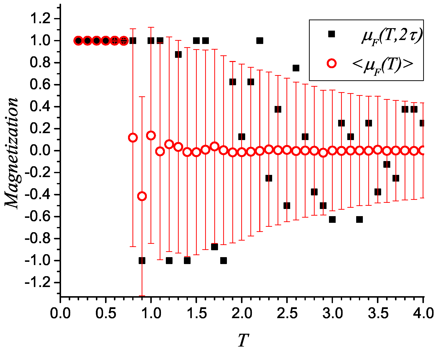
Figure 4.
Simulations on lattices for different effective coordination numbers whose values are given in the inset: 2.000 corresponds to PBC; 1.875 to FBC; 1.75 to the dilution of the lattice according to the decoration proposed in Figure 5 where four pieces with have been withdrawn; 1.500 corresponds to a similar decoration with ; 1.00 corresponds to a similar decoration with . B means P when , and it represents F for all of the other cases. For clarity, not all curves are shown with error bars.

Figure 5.
Diluted lattice upon decoration: four sectors are removed to leave spins with a total of bonds; FBC are imposed to get . Other similar decorations are defined in the text and in the previous figure.
Figure 5.
Diluted lattice upon decoration: four sectors are removed to leave spins with a total of bonds; FBC are imposed to get . Other similar decorations are defined in the text and in the previous figure.

Figure 6.
Average absolute magnetization for lattices of different sizes showing the tails for the artificial remnant magnetization induced by forced ergodicity breaking. The inset shows the decrease with the size of the number of magnetization reversal within 50,000 measurements after equilibration. For clarity, error bars are given for only.

Figure 7.
Instantaneous magnetization after MCSs of equilibration for the lattice , , with FBC at . Measurements are separated by 20 MCSs.
Figure 7.
Instantaneous magnetization after MCSs of equilibration for the lattice , , with FBC at . Measurements are separated by 20 MCSs.
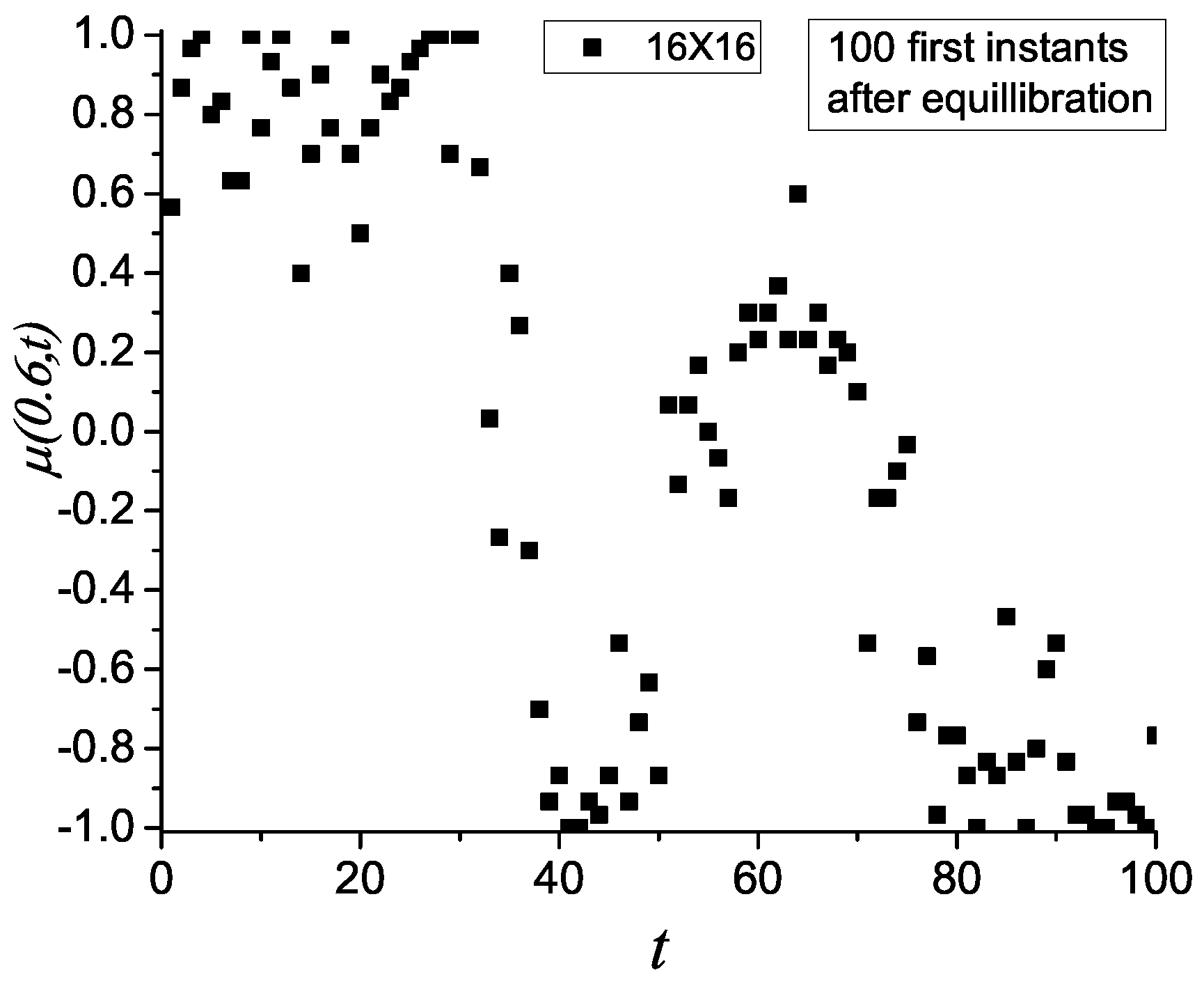
Figure 8.
Magnetization for different systems based on layers where the effective coordination number varies as given in the inset: 1.50 (one layer ; B = F); 2.0 (two layers ; B = F); 2.167 (three layers ; B = F); 2.25 (four layers ; B = F); 2.50 (four layers ; B = 2F + 1P); 2.75 (four layers ; B = 1F + 2P); 3.0 (four layers ; B = P) (the first curve is truly 2D, and part of it was already included in Figure 2; it is given here for completeness and comparison purposes).
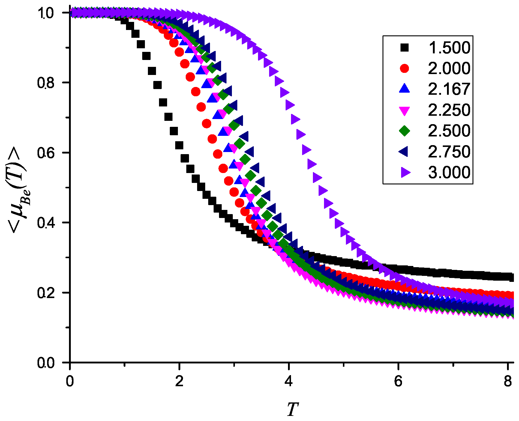
Figure 9.
Sensitive temperature from a magnetic ordered to a disordered phase for the q-states clock model as a function of . A square lattice with FBC is used. Measurements are obtained after MCSs for averaging.
Figure 9.
Sensitive temperature from a magnetic ordered to a disordered phase for the q-states clock model as a function of . A square lattice with FBC is used. Measurements are obtained after MCSs for averaging.

Table 1.
Coefficients for periodic boundary condition (PBC) configurations of a given energy and magnetization . The first column gives n; the second column gives the corresponding energy ; the following columns give the number of configurations for that energy (row) and magnetization (column). This table is symmetric and should be extended to the left by means of the symmetry properties so as to include the 8 negative values of the magnetization following Equations (10) and (12).
| k= | 9 | 8 | 7 | 6 | 5 | 4 | 3 | 2 | 1 | |
|---|---|---|---|---|---|---|---|---|---|---|
| n | 0 | 2 | 4 | 6 | 8 | 10 | 12 | 14 | 16 | |
| 15 | 32 | 2 | ||||||||
| 14 | 24 | 16 | ||||||||
| 13 | 20 | 64 | ||||||||
| 12 | 16 | 120 | 96 | 56 | ||||||
| 11 | 12 | 576 | 512 | 64 | ||||||
| 10 | 8 | 2112 | 1392 | 768 | 128 | |||||
| 9 | 4 | 3264 | 3136 | 1568 | 448 | |||||
| 8 | 0 | 4356 | 3680 | 2928 | 1248 | 228 | ||||
| 7 | −4 | 1600 | 1920 | 1824 | 1664 | 576 | ||||
| 6 | −8 | 768 | 624 | 704 | 688 | 736 | 208 | |||
| 5 | −12 | 64 | 96 | 192 | 256 | 256 | ||||
| 4 | −16 | 8 | 24 | 96 | 88 | |||||
| 3 | −20 | 32 | ||||||||
| 2 | −24 | 16 | ||||||||
| 1 | −32 | 1 |
Table 2.
Coefficients for free boundary condition (FBC) configurations of a given energy and magnetization . The first column gives n; the second column gives the corresponding energy ; the following columns give the number of configurations for that energy (row) and magnetization (column). This table is symmetric and should be extended to the left so as to include the 8 negative values of the magnetization following Equations (9) and (11).
| k= | 9 | 8 | 7 | 6 | 5 | 4 | 3 | 2 | 1 | |
|---|---|---|---|---|---|---|---|---|---|---|
| n | = 0 | 2 | 4 | 6 | 8 | 10 | 12 | 14 | 16 | |
| 23 | 24 | 2 | ||||||||
| 22 | 20 | 4 | ||||||||
| 21 | 18 | 16 | 8 | |||||||
| 20 | 16 | 36 | 16 | 2 | ||||||
| 19 | 14 | 80 | 56 | 16 | ||||||
| 18 | 12 | 192 | 148 | 48 | ||||||
| 17 | 10 | 384 | 296 | 112 | 8 | |||||
| 16 | 8 | 814 | 596 | 272 | 44 | |||||
| 15 | 6 | 1360 | 1096 | 552 | 136 | |||||
| 14 | 4 | 1800 | 1608 | 864 | 288 | 12 | ||||
| 13 | 2 | 2256 | 1984 | 1296 | 512 | 72 | ||||
| 12 | 0 | 2320 | 2044 | 1604 | 740 | 188 | ||||
| 11 | −2 | 1680 | 1616 | 1352 | 872 | 304 | 8 | |||
| 10 | −4 | 1008 | 1032 | 880 | 804 | 392 | 60 | |||
| 9 | −6 | 544 | 584 | 592 | 520 | 368 | 128 | |||
| 8 | −8 | 270 | 236 | 286 | 260 | 256 | 144 | 2 | ||
| 7 | −10 | 80 | 72 | 96 | 120 | 144 | 112 | 24 | ||
| 6 | −12 | 24 | 36 | 20 | 48 | 68 | 64 | 44 | ||
| 5 | −14 | 8 | 16 | 16 | 8 | 32 | 32 | |||
| 4 | −16 | 4 | 8 | 12 | 10 | 4 | ||||
| 3 | −18 | 8 | 8 | |||||||
| 2 | −20 | 4 | ||||||||
| 1 | −24 | 1 |
© 2017 by the authors. Licensee MDPI, Basel, Switzerland. This article is an open access article distributed under the terms and conditions of the Creative Commons Attribution (CC BY) license (http://creativecommons.org/licenses/by/4.0/).
Share and Cite
MDPI and ACS Style
Vogel, E.E.; Vargas, P.; Saravia, G.; Valdes, J.; Ramirez-Pastor, A.J.; Centres, P.M. Thermodynamics of Small Magnetic Particles. Entropy 2017, 19, 499. https://doi.org/10.3390/e19090499
AMA Style
Vogel EE, Vargas P, Saravia G, Valdes J, Ramirez-Pastor AJ, Centres PM. Thermodynamics of Small Magnetic Particles. Entropy. 2017; 19(9):499. https://doi.org/10.3390/e19090499
Chicago/Turabian StyleVogel, Eugenio E., Patricio Vargas, Gonzalo Saravia, Julio Valdes, Antonio Jose Ramirez-Pastor, and Paulo M. Centres. 2017. "Thermodynamics of Small Magnetic Particles" Entropy 19, no. 9: 499. https://doi.org/10.3390/e19090499
Note that from the first issue of 2016, this journal uses article numbers instead of page numbers. See further details here.