Sequential Change-Point Detection via Online Convex Optimization


H. Milton Stewart School of Industrial and Systems Engineering, Georgia Institute of Technology, Atlanta, GA 30332, USA
*
Author to whom correspondence should be addressed.
Entropy 2018, 20(2), 108; https://doi.org/10.3390/e20020108
Submission received: 1 September 2017
/
Revised: 2 December 2017
/
Accepted: 5 February 2018
/
Published: 7 February 2018
(This article belongs to the Special Issue Information Theory in Machine Learning and Data Science)
Abstract
:Sequential change-point detection when the distribution parameters are unknown is a fundamental problem in statistics and machine learning. When the post-change parameters are unknown, we consider a set of detection procedures based on sequential likelihood ratios with non-anticipating estimators constructed using online convex optimization algorithms such as online mirror descent, which provides a more versatile approach to tackling complex situations where recursive maximum likelihood estimators cannot be found. When the underlying distributions belong to a exponential family and the estimators satisfy the logarithm regret property, we show that this approach is nearly second-order asymptotically optimal. This means that the upper bound for the false alarm rate of the algorithm (measured by the average-run-length) meets the lower bound asymptotically up to a log-log factor when the threshold tends to infinity. Our proof is achieved by making a connection between sequential change-point and online convex optimization and leveraging the logarithmic regret bound property of online mirror descent algorithm. Numerical and real data examples validate our theory.
1. Introduction
Sequential analysis is a classic topic in statistics concerning online inference from a sequence of observations. The goal is to make statistical inference as quickly as possible, while controlling the false-alarm rate. An important sequential analysis problem commonly studied is sequential change-point detection [1]. It arises from various applications including online anomaly detection, statistical quality control, biosurveillance, financial arbitrage detection and network security monitoring (see, e.g., [2,3,4]).
We are interested in the sequential change-point detection problem with known pre-change parameters but unknown post-change parameters. Specifically, given a sequence of samples , , …, we assume that they are independent and identically distributed (i.i.d.) with certain distribution parameterized by , and the values of are different before and after some unknown time called the change-point. We further assume that the parameters before the change-point are known. This is reasonable since usually it is relatively easy to obtain the reference data for the normal state, so that the parameters in the normal state can be estimated with good accuracy. After the change-point, however, the values of the parameters switch to some unknown values, which represent anomalies or novelties that need to be discovered.
1.1. Motivation: Dilemma of CUSUM and Generalized Likelihood Ratio (GLR) Statistics
Consider change-point detection with unknown post-change parameters. A commonly used change-point detection method is the so-called CUSUM procedure [4] that can be derived from likelihood ratios. Assume that before the change, the samples follow a distribution and after the change the samples follow another distribution . CUSUM procedure has a recursive structure: initialized with , the likelihood-ratio statistic can be computed according to , and a change-point is detected whenever exceeds a pre-specified threshold. Due to the recursive structure, CUSUM is memory and computation efficient since it does not need to store the historical data and only needs to record the value of . The performance of CUSUM depends on the choice of the post-change parameter ; in particular, there must be a well-defined notion of “distance” between and . However, the choice of is somewhat subjective. Even if in practice a reasonable choice of is the “smallest” change-of-interest, in the multi-dimensional setting, it is hard to define what the “smallest” change would mean. Moreover, when the assumed parameter deviates significantly from the true parameter value, CUSUM may suffer a severe performance degradation [5].
An alternative approach is the Generalized Likelihood Ratio (GLR) statistic based procedure [6]. The GLR statistic finds the maximum likelihood estimate (MLE) of the post-change parameter and plugs it back into the likelihood ratio to form the detection statistic. To be more precise, for each hypothetical change-point location k, the corresponding post-change samples are . Using these samples, one can form the MLE denoted as . Without knowing whether the change occurs and where it occurs beforehand when forming the GLR statistic, we have to maximize k over all possible change locations. The GLR statistic is given by , and a change is announced whenever it exceeds a pre-specified threshold. The GLR statistic is more robust than CUSUM [7], and it is particularly useful when the post-change parameter may vary from one situation to another. In simple cases, the MLE may have closed-form expressions and may be evaluated recursively. For instance, when the post-change distribution is Gaussian with mean [8], , and . However, in more complex situations, in general MLE does not have recursive form and cannot be evaluated using simple summary statistics. One such instance is given in Section 1.2. Another instance is when there is a constraint on the MLE such as sparsity. In these cases, one has to store historical data and recompute the MLE whenever there is new data, which is not memory efficient nor computational efficient. For these cases, as a remedy, the window-limited GLR is usually considered, where only the past w samples are stored and the maximization is restricted to be over . However, even with the window-limited GLR, one still has to recompute using historical data whenever the new data are added.
Besides CUSUM or GLR, various online change-point detection procedures using one-sample updates have been considered, which replace with the MLE with a simple recursive estimator. The one-sample update estimate takes the form of for some function h that uses only the most recent data and the previous estimate. Then the estimates are plugged into the likelihood ratio statistic to perform detection. Online convex optimization algorithms (such as online mirror descent) are natural approach to construct these estimators (see, e.g., [9,10]). Such a scheme provides a more versatile approach to developing a detecting procedure for complex situations, where the exact MLE does not have a recursive form or even a closed-form expression. The one-sample update enjoys efficient computation, as information from the new data can be incorporated via low computational cost update. It is also memory efficient since the update only needs the most recent sample. The one sample update estimators may not correspond to the exact MLE, but they tend to result in good detection performance. However, in general there is no performance guarantees for such an approach. This is the question we aim to address in this paper.
1.2. Application Scenario: Social Network Change-Point Detection
The widespread use of social networks (such as Twitter) leads to a large amount of user-generated data generated continuously. One important aspect is to detect change-points in streaming social network data. These change-points may represent the collective anticipation of response to external events or system “shocks” [11]. Detecting such changes can provide a better understanding of patterns of social life. In social networks, a common form of the data is discrete events over continuous time. As a simplification, each event contains a time label and a user label in the network. In our prior work [12], we model discrete events using network point processes, which capture the influence between users through an influence matrix. We then cast the problem as detecting changes in an influence matrix, assuming that the influence matrix in the normal state (before the change) can be estimated from the reference data. After the change, the influence matrix is unknown (since it represents an anomaly) and has to be estimated online. Due to computational burden and memory constraint, since the scale of the network tends to be large, we do not want to store the entire historical data and rather compute the statistic in real-time. A simulated example to illustrate this case is shown later in Section 4.4.
1.3. Contributions
This paper has two main contributions. First, we present a general approach based on online convex optimization (OCO) for constructing the estimator for the one-sided sequential hypothesis test and the sequential change-point detection, in the non-anticipative approach of [8] if the MLE cannot be computed in a convenient recursive form.
Second, we provide a proof of the near second-order asymptotic optimality of this approach when a “logarithmic regret property” is satisfied and when the distributions are from an exponential family. The nearly second-order asymptotic optimality [4] means that the upper bound for performance matches the lower bound up to a log-log factor as the false-alarm rate tends to zero. Inspired by the existing connection between sequential analysis and online convex optimization in [13,14], we prove the near optimality leveraging the logarithmic regret property of online mirror descent (OMD) and the lower bound established in statistical sequential change-point literature [4,15]. More precisely, we provide a general upper bound for the one-sided sequential hypothesis test and change-point detection procedures with the one-sample update schemes. The upper bound explicitly captures the impact of estimation on detection by an estimation algorithm dependent factor. This factor shows up as an additional term in the upper bound for the expected detection delay, and it corresponds to the regret incurred by the one-sample update estimators. This establishes an interesting linkage between sequential change-point detection and online convex optimization. Although both fields, sequential change-point detection and online convex optimization, study sequential data, the precise connection between them is not clear, partly because the performance metrics are different: the former is concerned with the tradeoff between average run length and detection delay, whereas the latter focuses on bounding the cumulative loss incurred by the sequence of estimators through a regret bound [14,16]. Synthetic examples validate the performances of one sample update schemes. Here we focus on OMD estimators, but the results can be generalized to other OCO schemes such as the online gradient descent.
1.4. Literature and Related Work
Sequential change-point detection is a classic subject with an extensive literature. Much success has been achieved when the pre-change and post-change distributions are exactly specified. For example, the CUSUM procedure [17] with first-order asymptotic optimality [18] and exact optimality [19] in the minimax sense, and the Shiryayev-Roberts (SR) procedure [20] derived based on Bayesian principle that also enjoys various optimality properties. Both CUSUM and SR procedures rely on likelihood ratios between the specified pre-change and post-change distributions.
There are two main approaches in dealing with the unknown post-change parameters. The first one is a GLR approach [7,21,22,23,24], and the second is a mixture approach [15,25]. The GLR statistic enjoys certain optimality properties, but it can not be computed recursively in many cases [23]. To address the infinite memory issue, [7,21] studied the window-limited GLR procedure. The main advantage of the mixture approach is that it allows an easy evaluation of a threshold that guarantees the desired false alarm constraint. A disadvantage of this approach is that sometimes there may not be a natural way of selecting the weight function, in particular when there is no conjugate prior. This motivated a third approach to this problem, which was proposed first by Robbins and Siegmund in the context of hypothesis testing, and then Lorden and Pollak [8] in the sequential change detection problem. This approach replaces the unknown parameter with some non-anticipating estimator, which can be easier to find even if there is no conjugate prior, as in the Gamma example considered in [8,25]. This work developed a modified SR procedure by introducing a prior distribution to the unknown parameters. While the non-anticipating estimator approach [8,24] enjoys recursive and thus efficient computation for the likelihood ratio based detection statistics, their approaches to constructing recursive estimators (based on MLE or method-of-moments) cannot be easily extended to more complex cases (for instance, multi-dimensional parameters with constraints). Here, we consider a general and convenient approach for constructing non-anticipating estimators based on online convex optimization which is particularly useful for these complex cases. Our work provides an alternative proof for the nearly second-order asymptotic optimality by building a connection to online convex optimization and leveraging the regret bound type of results [14]. For one-dimensional Gaussian mean shift without any constraint, we replicate the second-order asymptotic optimality, namely, Theorem 3.3 in [24]. Recent work [26] also treats the problem when the pre-change distribution has unknown parameters.
Another related problem is sequential joint estimation and detection, but the goal is different in that one aims to achieve both good detection and good estimation performance, whereas in our setting, estimation is only needed for computing the detection statistics. These works include [27] and [28], which study the joint detection and estimation problem of a specific form that arises from many applications such as spectrum sensing [29], image observations [30], and MIMO radar [31]: a linear scalar observation model with Gaussian noise, and under the alternative hypothesis there is an unknown multiplicative parameter. The paper of [27] demonstrates that solving the joint problem by treating detection and estimation separately with the corresponding optimal procedure does not yield an overall optimum performance, and provides an elegant closed-form optimal detector. Later on [28] generalizes the results. There are also other approaches solving the joint detection-estimation problem using multiple hypotheses testing [30,32] and Bayesian formulations [33].
Related work using online convex optimization for anomaly detection includes [9], which develops an efficient detector for the exponential family using online mirror descent and proves a logarithmic regret bound, and [10], which dynamically adjusts the detection threshold to allow feedbacks about whether decision outcome. However, these works consider a different setting that the change is a transient outlier instead of a persistent change, as assumed by the classic statistical change-point detection literature. When there is persistent change, it is important to accumulate “evidence” by pooling the post-change samples (our work considers the persistent change).
Extensive work has been done for parameter estimation in the online-setting. This includes online density estimation over the exponential family by regret minimization [9,10,16], sequential prediction of individual sequence with the logarithm loss [13,34], online prediction for time series [35], and sequential NML (SNML) prediction [34] which achieves the optimal regret bound. Our problem is different from the above, in that estimation is not the end goal; one only performs parameter estimation to plug them back into the likelihood function for detection. Moreover, a subtle but important difference of our work is that the loss function for online detecting estimation is , whereas our loss function is in order to retain the martingale property, which is essential to establish the nearly second-order asymptotic optimality.
2. Preliminaries
Assume a sequence of i.i.d. random variables with a probability density function of a parametric form . The parameter may be unknown. Consider two related problems: one-sided sequential hypothesis test and sequential change-point detection. The detection statistic relies on a sequence estimator constructed using online mirror descent. The OMD uses simple one-sample update: the update from to only uses the current sample . This is the main difference from the traditional generalized likelihood ratio (GLR) statistic [7], where each is estimated using historical samples. In the following, we present detailed descriptions for two problems. We will consider exponential family distributions and present our non-anticipating estimator based on the one-sample estimate.
2.1. One-Sided Sequential Hypothesis Test
First, we consider a one-sided sequential hypothesis test where the goal is only to reject the null hypothesis. This is a special case of the change-detection problem where the change-point can be either 0 or ∞ (meaning it never occurs). Studying this special case will given us an important intermediate step towards solving the sequential change-detection problem.
Consider the null hypothesis versus the alternative . Hence, the parameter under the alternative distribution is unknown. The classic approach to solve this problem is the one-sided sequential probablity-ratio test (SPRT) [36]: at each time, given samples , the decision is either to reject or taking more samples if the rejection decision can not be made confidently. Here, we introduce a modified one-sided SPRT with a sequence of non-anticipating plug-in estimators:
Define the test statistic at time t as
The test statistic has a simple recursive implementation:
Define a sequence of -algebras where . The test statistic has the martingale property due to its non-anticipating nature: , where the expectation is taken when are i.i.d. random variables drawn from . The decision rule is a stopping time
where is a pre-specified threshold. We reject the null hypothesis whenever the statistic exceeds the threshold. The goal is to reject the null hypothesis using as few samples as possible under the false-alarm rate (or Type-I error) constraint.
2.2. Sequential Change-Point Detection
Now we consider the sequential change-point detection problem. A change may occur at an unknown time which alters the underlying distribution of the data. One would like to detect such a change as quickly as possible. Formally, change-point detection can be cast into the following hypothesis test:
Here we assume an unknown to represent the anomaly. The goal is to detect the change as quickly as possible after it occurs under the false-alarm rate constraint. We will consider likelihood ratio based detection procedures adapted from two types of existing ones, which we call the adaptive CUSUM (ACM), and the adaptive SRRS (ASR) procedures.
For change-point detection, the post-change parameter is estimated using post-change samples. This means that, for each putative change-point location before the current time , the post-change samples are ; with a slight abuse of notation, the post-change parameter is estimated as
Therefore, for , becomes defined in (2) for the one-sided SPRT. Initialize with . The likelihood ratio at time t for a hypothetical change-point location k is given by
where can be computed recursively similar to (2).
Since we do not know the change-point location , from the maximum likelihood principle, we take the maximum of the statistics over all possible values of k. This gives the ACM procedure:
where is a pre-specified threshold. Similarly, by replacing the maximization over k in (7) with summation, we obtain the following ASR procedure [8], which can be interpreted as a Bayesian statistic similar to the Shiryaev-Roberts procedure.
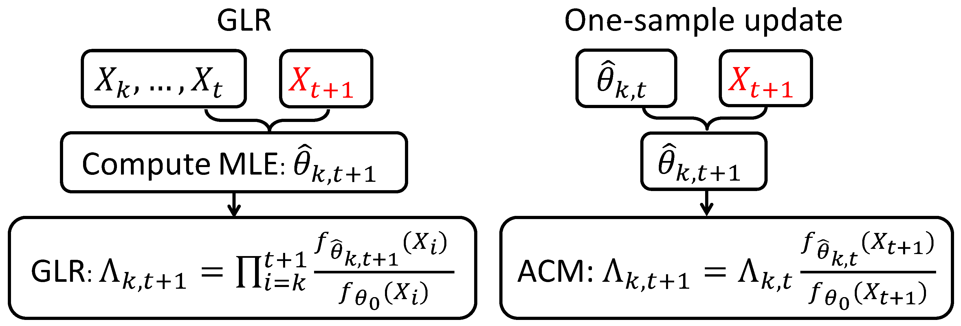
where is a pre-specified threshold. The computations of and estimator , are discussed later in Section 2.4. For a fixed k, the comparison between our methods and GLR is illustrated in Figure 1.
Remark 1.
In practice, to prevent the memory and computation complexity from blowing up as time t goes to infinity, we can use window-limited version of the detection procedures in (7) and (8). The window-limited versions are obtained by replacing with in (7) and by replacing with in (8). Here w is a prescribed window size. Even if we do not provide theoretical analysis to the window-limited versions, we refer the readers to [7] for the choice of w the window-limited GLR procedures.
2.3. Exponential Family
In this paper, we focus on being the exponential family for the following reasons: (i) exponential family [10] represents a very rich class of parametric and even many nonparametric statistical models [37]; (ii) the negative log-likelihood function for exponential family is convex, and this allows us to perform online convex optimization. Some useful properties of the exponential family are briefly summarized below, and full proofs can be found in [10,38].
Consider an observation space equipped with a sigma algebra and a sigma finite measure H on . Assume the number of parameters is d. Let denote the transpose of a vector or matrix. Let be an H-measurable function . Here corresponds to the sufficient statistic for . Let denote the parameter space in . Let be a set of probability distributions with respect to the measure H. Then, is said to be a multivariate exponential family with natural parameter , if the probability density function of each with respect to H can be expressed as In the definition, the so-called log-partition function is given by
To make sure a well-defined probability density, we consider the following two sets for parameters:
and
Note that is -strongly convex over . Its gradient corresponds to , and the Hessian corresponds to the covariance matrix of the vector . Therefore, is positive semidefinite and is convex. Moreover, is a Legendre function, which means that it is strongly convex, continuous differentiable and essentially smooth [38]. The Legendre-Fenchel dual is defined as
The mappings is an inverse mapping of [39]. Moreover, if is a strongly convex function, then .
A general measure of proximity used in the OMD is the so-called Bregman divergence , which is a nonnegative function induced by a Legendre function F (see, e.g., [10,38]) defined as
For exponential family, a natural choice of the Bregman divergence is the Kullback-Leibler (KL) divergence. Define as the expectation when X is a random variable with density and as the KL divergence between two distributions with densities and for any . Then
It can be shown that, for exponential family, Using the definition (9), this means that
is a Bregman divergence. This property is useful to constructing mirror descent estimator for the exponential family [39,40].
2.4. Online Convex Optimization (OCO) Algorithms for Non-Anticipating Estimators
Online convex optimization (OCO) algorithms [14] can be interpreted as a player who makes sequential decisions. At the time of each decision, the outcomes are unknown to the player. After committing to a decision, the decision maker suffers a loss that can be adversarially chosen. An OCO algorithm makes decisions, which, based on the observed outcomes, minimizes the regret that is the difference between the total loss that has incurred relative to that of the best fixed decision in hindsight. To design non-anticipating estimators, we consider OCO algorithms with likelihood-based regret functions. We iteratively estimate the parameters at the time when one new observation becomes available based on the maximum likelihood principle, and hence the loss incurred corresponds to the negative log-likelihood of the new sample evaluated at the estimator , which corresponds to the log-loss in [13]. Given samples , the regret for a sequence of estimators generated by a likelihood-based OCO algorithm is defined as
Below we omit the superscript occasionally for notational simplicity.
In this paper, we consider a generic OCO procedure called the online mirror descent algorithms (OMD) [14,41]. Next, we discuss how to construct the non-anticipating estimators in (1), and in (5) using OMD. The main idea of OMD is the following. At each time step, the estimator is updated using the new sample , by balancing the tendency to stay close to the previous estimate against the tendency to move in the direction of the greatest local decrease of the loss function. For the loss function defined above, a sequence of OMD estimator is constructed by
where is defined in (11). Here is a closed convex set, which is problem-specific and encourages certain parameter structure such as sparsity.
Remark 2.
There is an equivalent form of OMD, presented as the original formulation in [40]. The equivalent form is sometimes easier to use for algorithm development, and it consists of four steps: (1) compute the dual variable: ; (2) perform the dual update: ; (3) compute the primal variable: ; (4) perform the projected primal update: . The equivalence between the above form for OMD and the nonlinear projected subgradient approach in (13) is proved in [39]. We adopt this approach when deriving our algorithm and follow the same strategy as [9]. Algorithm 1 summarizes the steps [42].
For strongly convex loss function, the regret of many OCO algorithms, including the OMD, has the property that for some constant C (depend on and ) and any positive integer n [10,43]. Note that for exponential family, the loss function is the negative log-likelihood function, which is strongly convex over . Hence, we can have the logarithmic regret property.
| Algorithm 1 Online mirror-descent for non-anticipating estimators. |
| Require: Exponential family specifications and ; initial parameter value ; sequence of data ; a closed, convex set for parameter ; a decreasing sequence of strictly positive step-sizes. |
| 1: . {Initialization} |
| 2: for all do |
| 3: Acquire a new observation |
| 4: Compute loss |
| 5: Compute likelihood ratio |
| 6: , {Dual update} |
| 7: |
| 8: {Projected primal update} |
| 9: end for |
| 10: return and . |
3. Nearly Second-Order Asymptotic Optimality of One-Sample Update Schemes
Below we prove the nearly second-order asymptotic optimality of the one-sample update schemes. More precisely, the nearly second-order asymptotic optimality means that the algorithm obtains the lower performance bound asymptotically up to a log-log factor in the false-alarm rate, as the false-alarm rate tends to zero (in many cases the log-log factor is a small number).
We first introduce some necessary notations. Denote and as the probability measure and the expectation when the change occurs at time and the post-change parameter is , i.e., when are i.i.d. random variables with density and are i.i.d. random variables with density . Moreover, let and denote the probability measure when there is no change, i.e., are i.i.d. random variables with density . Finally, let denote the -algebra generated by for .
3.1. “One-Sided” Sequential Hypothesis Test
Recall that the decision rule for sequential hypothesis test is a stopping time defined in (3). The two standard performance metrics are the false-alarm rate, denoted as , and the expected detection delay (i.e., the expected number of samples needed to reject the null), denoted as . A meaningful test should have both small and small . Usually, one adjusts the threshold b to control the false-alarm rate to be below a certain level.
Our main result is the following. As has been observed by [23], there is a loss in the statistical efficiency by using one-sample update estimators relative to the GLR approach using the entire samples in the past. The theorem below shows that this loss corresponds to the expected regret given in (12).
Theorem 1 (Upper bound for OCO based SPRT).
Let be a sequence of non-anticipating estimators generated by an OCO algorithm . As ,
Here is a term upper-bounded by an absolute constant as .
The main idea of the proof is to decompose the statistic defining , , into a few terms that form martingales, and then invoke the Wald’s Theorem for the stopped process.
Remark 3.
The inequality (14) is valid for a sequence of non-anticipating estimators generated by an OCO algorithm. Moreover, (14) gives an explicit connection between the expected detection delay for the one-sided sequential hypothesis testing (left-hand side of (14)) and the regret for the OCO (the second term on the right-hand side of (14)). This illustrates clearly the impact of estimation on detection by an estimation algorithm dependent factor.
Note that in the statement of the Theorem 1, the stopping time appears on the right-hand side of the inequality (14). For OMD, the expected sample size is usually small. By comparing with specific regret bound , we can bound as discussed in Section 4. The most important case is that when the estimation algorithm has a logarithmic expected regret. For the exponential family, as shown in Section 3.3, Algorithm 1 can achieve for any positive integer n. To obtain a more specific order of the upper bound for when b grows, we establish an upper bound for as a function of b, to obtain the following Corollary 1.
Corollary 1.
Let be a sequence of non-anticipating estimators generated by an OCO algorithm . Assume that for any positive integer n and some constant , we have
Here is a vanishing term as .
Corollary 1 shows that other than the well known first-order approximation [8,18], the expected detection delay is bounded by an additional term that is on the order of if the estimation algorithm has a logarithmic regret. This term plays an important role in establishing the optimality properties later. To show the optimality properties for the detection procedures, we first select a set of detection procedures with false-alarm rates lower than a prescribed value, and then prove that among all the procedures in the set, the expected detection delays of our proposed procedures are the smallest. Thus, we can choose a threshold b to uniformly control the false-alarm rate of .
Lemma 1 (false-alarm rate of ).
Let be any sequence of non-anticipating estimators. For any , .
Lemma 1 shows that as b increases the false-alarm rate of decays exponentially fast. We can set to make the false-alarm rate of less than some . Next, leveraging an existing lower bound for general SPRT presented in Section 5.5.1.1 in [4], we establish the nearly second-order asymptotic optimality of OMD based SPRT as follows:
Corollary 2 (Nearly second-order optimality of OCO based SPRT).
Let be a sequence of non-anticipating estimators generated by an OCO algorithm . Assume that for any positive integer n and some constant . Define a set . For , due to Lemma 1, . For such a choice, is nearly second-order asymptotic optimal in the sense that for any , as ,
The result means that, compared with any procedure (including the optimal procedure) calibrated to have a false-alarm rate less than , our procedure incurs an at most increase in the expected detection delay, which is usually a small number. For instance, even for a conservative case when we set to control the false-alarm rate, the number is .
3.2. Sequential Change-Point Detection
Now we proceed the proof by leveraging the close connection [18] between the sequential change-point detection and the one-sided hypothesis test. For sequential change-point detection, the two commonly used performance metrics [4] are the average run length (ARL), denoted by ; and the maximal conditional average delay to detection (CADD), denoted by . ARL is the expected number of samples between two successive false alarms, and CADD is the expected number of samples needed to detect the change after it occurs. A good procedure should have a large ARL and a small CADD. Similar to the one-sided hypothesis test, one usually choose the threshold large enough so that ARL is larger than a pre-specified level.
Similar to Theorem 1, we provide an upper bound for the CADD of our ASR and ACM procedures.
Theorem 2.
To prove Theorem 2, we relate the ASR and ACM procedures to the one-sided hypothesis test and use the fact that when the measure is known, is attained at for both the ASR and the ACM procedures. Above, we may apply a similar argument as in Corollary 1 to remove the dependence on on the right-hand-side of the inequality. We establish the following lower bound for the ARL of the detection procedures, which is needed for proving Corollary 3:
Lemma 2 (ARL).
Lemma 2 shows that given a required lower bound for ARL, we can choose to make the ARL be greater than . This is consistent with earlier works [8,25] which show that the smallest threshold b such that is approximate . However, the bound in Lamma 2 is not tight, since in practice we can set for some to ensure that ARL is greater than .
Combing the upper bound in Theorem 2 with an existing lower bound for the CADD of SRRS procedure in [15], we obtain the following optimality properties.
Corollary 3 (Nearly second-order asymptotic optimality of ACM and ASR).
Consider the change-point detection procedure in (7) and in (8). For any fixed k, let be a sequence of non-anticipating estimators generated by an OCO algorithm . Assume that for any positive integer n and some constant . Let . Define . For , due to Lemma 2, both and belong to . For such b, both and are nearly second-order asymptotic optimal in the sense that for any
A similar expression holds for .
The result means that, compared with any procedure (including the optimal procedure) calibrated to have a fixed ARL larger than , our procedure incurs an at most increase in the CADD. Comparing (18) with (16), we note that the ARL plays the same role as because is roughly the false-alarm rate for sequential change-point detection [18].
3.3. Example: Regret Bound for Specific Cases
In this subsection, we show that the regret bound can be expressed as a weighted sum of Bregman divergences between two consecutive estimators. This form of is useful to show the logarithmic regret for OMD. The following result comes as a modification of [16].
Theorem 3.
Assume that are i.i.d. random variables with density function . Let in Algorithm 1. Assume that are obtained using Algorithm 1 and (defined in step 7 and 8 of Algorithm 1) for any . Then for any and ,
where , for some .
Next, we use Theorem 3 on a concrete example. The multivariate normal distribution, denoted by , is parametrized by an unknown mean parameter and a known covariance matrix ( is a identity matrix). Following the notations in Section 2.3, we know that , , for any , , and , where denotes the determinant of a matrix, and H is a probability measure under which the sample follows ). When the covariance matrix is known to be some , one can “whiten” the vectors by multiplying to obtain the situation here.
Corollary 4 (Upper bound for the expected regret, Gaussian).
Assume are i.i.d. following with some . Assume that are obtained using Algorithm 1 with and . For any , we have that for some constant that depends on θ,
The following calculations justify Corollary 4, which also serve as an example of how to use regret bound. First, the assumption in Theorem 3 is satisfied for the following reasons. Consider is the full space. According to Algorithm 1, using the non-negativity of the Bregman divergence, we have Then the regret bound can be written as
Since the step-size , the second term in the above equation can be written as:
Combining above, we have
Finally, since for any , we obtain the desired result. Thus, with i.i.d. multivariate normal samples, the expected regret grows logarithmically with the number of samples.
Using the similar calculations, we can also bound the expected regret in the general case. As shown in the proof above for Corollary 4, the dominating term for can be rewritten as
where is a convex combination of and . For an arbitrary distribution, the term can be viewed as a local normal distribution with the changing curvature . Thus, it is possible to prove case-by-case the -style bounds by making more assumptions about the distributions. Recall the notation in Section 2.3 such that is -strongly convex over . Let denote the norm. Moreover, we assume that the true parameter belongs to a set that is a closed and convex subset of such that for some constant M. Thus, one can show that is not only -strongly convex but also M-strongly smooth over . Theorem 3 in [10] shows that for all and , consider that is obtained by OMD, then
Therefore, for any bounded distributions within the exponential family, we achieve a logarithmic regret. This logarithmic regret is valid for Bernoulli distribution, Beta distribution and some truncated versions of classic distributions (e.g., truncated Gaussian distribution, truncated Gamma distribution and truncated Geometric distribution analyzed in [44]).
4. Numerical Examples
In this section, we present some synthetic examples to demonstrate the good performance of our methods. We will focus on ACM and ASR for sequential change-point detection. In the following, we consider the window-limited versions (see Remark 1) of ACM and ASR with window size . Recall that when the measure is known, is attained at for both ASR and ACM procedures (a proof can be found in the proof of Theorem 2). Therefore, in the following experiments we define the expected detection delay (EDD) as for a stopping time T. To compare the performance between different detection procedures, we determine the threshold for each detection procedure by Monte-Carlo simulations such that the ARL for each procedure is about . Below, we denote , and as the norm, norm and norm defined as the number of non-zero entries, respectively. The following experiments are all run on the same Macbook Air with an Intel i7 Core CPU.
4.1. Detecting Sparse Mean-Shift of Multivariate Normal Distribution
We consider detect the sparse mean shift for multivariate normal distribution. Specifically, we assume that the pre-change distribution is and the post-change distribution is for some unknown , where s is called the sparsity of the mean shift. Sparse mean shift detection is of particular interest in sensor networks [45,46]. For this Gaussian case, the Bregman divergence is given by Therefore, the projection onto in Algorithm 1 is a Euclidean projection onto a convex set, which in many cases can be implemented efficiently. As a frequently used convex relaxation of the -norm ball, we set (it is known that imposing an constraint leads to sparse solution; see, e.g., [47]). Then, the projection onto ball can be computed very efficiently via a simple soft-thresholding technique [48].
Two benchmark procedures are the CUSUM and the GLR. For the CUSUM procedure, we specify a nominal post-change mean, which is an all-one vector. If knowing the post-change mean is sparse, we can also use the shrinkage estimator presented in [49], which performs hard or soft thresholding of the estimated post-change mean parameter. Our procedures are and with and . In the following experiments, we run Monte Carlo trials to obtain each simulated EDD.
In the experiments, we set . The post-change distributions are , where entry of is 1 and others are 0, and the location of nonzero entries are random. Table 1 shows the EDDs versus the proportion p. Note that our procedures incur little performance loss compared with the GLR procedure and the CUSUM procedure. Notably, with performs almost the same as the GLR procedure and much better than the CUSUM procedure when p is small. This shows the advantage of projection when the true parameter is sparse.
4.2. Detecting the Scale Change in Gamma Distribution
We consider an example that detects the scale change in Gamma distributions. Assume that we observe a sequence of samples drawn from for some , with the probability density function given by (to avoid confusion with the parameter in Algorithm 1 we use to denote the Gamma function). The parameter is called the dispersion parameter that scales the loss and the divergences. For simplicity, we fix just like we fix the variance in the Gaussian case. The specifications in the Algorthm 1 are as follows: , , , , , and . Assume that the pre-change distribution is and the post-change distribution is for some unknown . We compare our algorithms with CUSUM, GLR and non-ancitipating estimator based on the method of moment (MOM) estimator in [8]. For the CUSUM procedure, we specify the post-change to be 2. The results are shown in Table 2. CUSUM fails to detect the change when , which is far away from the pre-specified post-change parameter . We can see that performance loss of the proposed ACM method compared with GLR and MOM is very small.
4.3. Communication-Rate Change Detection with Erdos-Rényi Model
Next, we consider a problem to detect the communication-rate change in a network, which is a model for social network data. Suppose we observe communication between nodes in a network over time, represented as a sequence of (symmetric) adjacency matrices of the network. At time t, if node i and node j communicates, then the adjacency matrix has 1 on the th and th entries (thus it forms an undirected graph). The nodes that do not communicate have 0 on the corresponding entries. We model such communication patterns using the Erdos-Renyi random graph model. Each edge has a fixed probability of being present or absent, independently of the other edges. Under the null hypothesis, each edge is a Bernoulli random variable that takes values 1 with known probability p and value 0 with probability . Under the alternative hypothesis, there exists an unknown time , after which a small subset of edges occur with an unknown and different probability .
In the experiments, we set and . For the pre-change parameters, we set for all . For the post-change parameters, we randomly select n out of the 190 edges, denoted by , and set for and for . As said before, let the change happen at time (since the upper bound for EDD is achieved at as argued in the proof of Theorem 2). To implement CUSUM, we specify the post-change parameters for all .
The results are shown in Table 3. Our procedures are better than CUSUM procedure when n is small since the post-change parameters used in CUSUM procedure is far from the true parameter. Compared with the GLR procedure, our methods have a small performance loss, and the loss is almost negligible as n approaches to .
Below are the specifications of Algorithm 1 in this case. For Bernoulli distribution with unknown parameter p, the natural parameter is equal to . Thus, we have , , , , and .
4.4. Point Process Change-Point Detection: Poisson to Hawkes Processes
In this example, to illustrate the situation in Section 1.2, we consider a case where a homogeneous Poisson process switches to a Hawkes process (see, e.g., [12]); this can be viewed as a simplest case in Section 1.2 with one node. We construct ACM and ASR procedures. In this case, the MLE for the unknown post-change parameter cannot be found in close-form, yet ACM and ASR can be easily constructed and give reasonably good performance, although our theory no longer holds in this case due to the lack of i.i.d. samples.
The Hawkes process can be viewed as a non-homogeneous Poisson process where the intensity is influenced by historical events. The data consist of a sequence of events occurring at times before a time horizon T: . Assume the intensity of the Poisson process is and there may exists a change-point such that the process changes. The null and alternative hypothesis tests are
where is a known baseline intensity, is unknown magnitude of the change, is the normalized kernel function with pre-specified parameter , which captures the influence from the past events. We treat the post-change influence parameter as unknown since it represents an anomaly.
We first use a sliding window to convert the event times into a sequence of vectors with overlapping events. Assume of size of the sliding window is L. For a given scanning time , we map all the events in to a vector , , where is the number of events falling into the window. Note that can have different length for different i. Consider a set of scanning times . This maps the event times into a sequence of vectors of lengthes , , …, . These scanning times can be arbitrary; here we set them to be event times so that there are at least one sample per sliding window.
For a hypothetical change-point location k, it can be shown that the log-likelihood ratio (between the Hawkes process and the Poisson process) as a function of , is given by
Now based on this sliding window approach, we can approximate the original change-point detection problem as the following. Without change, are sampled from a Poisson process. Under the alternative, the change occurs at some time such that are sampled from a Poisson process, and are sampled from a Hawkes process with parameter , rather than a Poisson process. We define the estimator of , for assumed change-point location as follows
Now, consider , and keep w estimators: . The update for each estimator is based on stochastic gradient descent. By taking derivative with respect to , we have
Note that there is no close form expression for the MLE, which the solution to the above equation. We perform stochastic gradient descent instead
where is the step-size. Now we can apply the ACM and ASR procedures, by using the fact that and calculating using (19).
Table 4 shows the EDD for different . Here we choose the threshold such that ARL is 5000. We see that the scheme has a reasonably good performance, the detection delay decreases as the true signal strength increases.
5. Conclusions
In this paper, we consider sequential hypothesis testing and change-point detection with computationally efficient one-sample update schemes obtained from online mirror descent. We show that the loss of the statistical efficiency caused by the online mirror descent estimator (replacing the exact maximum likelihood estimator using the complete historical data) is related to the regret incurred by the online convex optimization procedure. The result can be generalized to any estimation method with logarithmic regret bound. This result sheds lights on the relationship between the statistical detection procedures and the online convex optimization.
Acknowledgments
This research was supported in part by National Science Foundation (NSF) NSF CCF-1442635, CMMI-1538746, NSF CAREER CCF-1650913 to Yao Xie. We would like to thank the anonymous reviewers to provide insightful comments.
Author Contributions
Yang Cao, Yao Xie, and Huan Xu conceived the idea and performed the theoretical part of the paper; Liyan Xie helped with numerical examples of the manuscript.
Conflicts of Interest
The authors declare no conflict of interest.
Appendix A. Proofs
Proof of Theorem 1.
In the proof, for the simplicity of notation we use N to denote . Recall is the true parameter. Define that
Then under the measure , is a random walk with i.i.d. increment. Then, by Wald’s identity (e.g., [1]) we have that
On the other hand, let denote the MLE based on . The key to the proof is to decompose the stopped process as a summation of three terms as follows:
Note that the first term of the decomposition on the right-hand side of (A2) is always non-positive since
Therefore we have
Now consider the third term in the decomposition (A2). Similar to the proof of equation (5.109) in [4], we claim that its expectation under measure is upper bounded by as . Next, we prove the claim. For any positive integer n, we further decompose the third term in (A2) as
where
and
The decomposition of (A3) consists of stochastic processes and , which are both -martingales with zero expectation, i.e., for any positive integer n. Since for exponential family, the log-partition function is bounded, by the inequalities for martingales [47] we have that
where and are two absolute constants that do not depend on n. Moreover, we observe that for all ,
Therefore, applying (A4), we have that and converge to 0 almost surely. Moreover, the convergence is -r-quickly for . We say that converges -r-quickly to a constant I if for all , where is the last time when leaves the interval (for more details, we refer the readers to Section 2.4.3 of [4]). Therefore, dividing both sides of (A3) by n, we obtain converges -1-quickly to .
For , we now define the last entry time
By the definition of -1-quickly convergence and the finiteness of , we have that for all . In the following, define a scaled threshold . Observe that conditioning on the event , we have that
Therefore, conditioning on the event , we have that . Hence, for any , we have
Since for any , from (A5) above, we have that the third term in (A2) is upper bounded by .
Proof of Corollary 1.
First, we can relate the expected regret at the stopping time to the expected stopping time, using the following chain of equalities and inequalities
where the first equality uses iterative expectation, the first inequality uses the assumption of the logarithmic regret in the statement of Corollary 1, and the second inequality is due to Jensen’s inequality. Let , and . Applying (A6), the upper bound in Equation (14) becomes . From this, we have . Taking logarithm on both sides and using the fact that for , . Therefore, we have that . Using this argument, we obtain
Note that a similar argument can be found in [49]. ☐
Next we will establish a few Lemmas useful for proving Theorem 2 for sequential detection procedures. Define a measure on under which the probability density of conditional on is . Then for any event , we have that . The following lemma shows that the restriction of to is well defined.
Lemma A1.
Let be the restriction of to . Then for any and any , .
Proof of Lemma 1.
To bound the term , we need take advantage of the martingale property of in (2). The major technique is the combination of change of measure and Wald’s likelihood ratio identity [1]. The proofs are a combination of the results in [23] and [8] and the reader can find a complete proof in [23]. For purpose of completeness we copy those proofs here.
Define the as the Radon-Nikodym derivative, where and are the restriction of and to , respectively. Then we have that for any (note that is defined in (2)). Combining the Lemma A1 and the Wald’s likelihood ratio identity, we have that>
where is an indicator function that is equal to 1 for any and is equal to 0 otherwise. By the definition of we have that . Taking in (A8) we prove that . ☐
Proof of Corollary 2.
Proof of Theorem 2.
From (A10), we have that for any ,
Therefore, to prove the theorem using Theorem 1, it suffices to show that
Using an argument similar to the remarks in [8], we have that the supreme of detection delay over all change locations is achieved by the case when change occurs at the first instance,
This is a slight modification (a small change on the subscripts) of the remarks in [8] but for the purpose of completeness and clearness we write the details in the following. Notice that since is known, for any , the distribution of under conditional on is the same as the distribution of under . Below, we use a renewal property of the ACM procedure. Define
Then we have that . However, for any . Therefore, conditioning on . So that for all ,
Thus, to prove (A9), it suffices to show that . To show this, define as the new stopping time that applies the one-sided sequential hypothesis testing procedure to data . Then we have that in fact , this relationship was developed in [18]. Thus, , and . ☐
Proof of Lemma 2.
This is a classic result proved by using the martingale property and the proof routine can be found in many textbooks such as [4]. First, rewrite as
Next, since
we have . So it suffices to show that , if . Define . Direct computation shows that
Therefore, is a -martingale with zero mean. Suppose that (otherwise the statement of proposition is trivial), then we have that
Equation (A11) leads to the fact that and the fact that conditioning on the event , we have that
Therefore, we can apply the optional stopping theorem for martingales, to obtain that . By the definition of , we have that . Therefore, if , we have that . ☐
Proof of Corollary 3.
Our Theorem 1 and the remarks in [15] show that the minimum worst-case detection delay, given a fixed ARL level , is given by
It can be shown that the infimum is attained by choosing as a weighted Shiryayev-Roberts detection procedure, with a careful choice of the weight over the parameter space . Combing (A12) with the right-hand side of (15), we prove the corollary. ☐
The following derivation borrows ideas from [16]. First, we derive concise forms of the two terms in the definition of in (12).
Lemma A2.
Assume that are i.i.d. random variables with density function , and assume decreasing step-size in Algorithm 1. Given generated by Algorithm 1. If for any , then for any null distribution parameter and ,
Moreover, for any ,
where .
By subtracting the expressions in (A13) and (A14), we obtain the following result which shows that the regret can be represented by a weighted sum of the Bregman divergences between two consecutive estimators.
Proof of Lemma A2.
By the definition of the Legendre-Fenchel dual function we have that for any . By this definition, and choosing , we have that for any
where we use the update rule in Line 6 of Algorithm 1 and the assumption to have the third equation. We define in the last equation. Now summing the terms in (A15), where the second term form a telescopic series, over i from 1 to t, we have that
Moreover, from the definition we have that
Taking the first derivative of with respect to and setting it to 0, we find , the stationary point, given by
Similarly, using the expression of the dual function, and plugging back into the equation, we have that
☐
Proof of Theorem 3.
By choosing the step-size for any in Algorithm 1, and assuming for any , we have by induction that
Subtracting (A13) by (A14), we obtain
The final equality is obtained by Taylor expansion. ☐
References
- Siegmund, D. Sequential Analysis: Tests and Confidence Intervals; Springer: Berlin, Germany, 1985. [Google Scholar]
- Chen, J.; Gupta, A.K. Parametric Statistical Change Point Analysis; Birkhauser: Basel, Switzerland, 2000. [Google Scholar]
- Siegmund, D. Change-points: From sequential detection to biologu and back. Seq. Anal. 2013, 23, 2–14. [Google Scholar] [CrossRef]
- Tartakovsky, A.; Nikiforov, I.; Basseville, M. Sequential Analysis: Hypothesis Testing and Changepoint Detection; CRC Press: Boca Raton, FL, USA, 2014. [Google Scholar]
- Granjon, P. The CuSum Algorithm—A Small Review. 2013. Available online: https://hal.archives-ouvertes.fr/hal-00914697 (accessed on 6 February 2018).
- Basseville, M.; Nikiforov, I.V. Detection of Abrupt Changes: Theory and Application; Prentice Hall Englewood Cliffs: Upper Saddle River, NJ, USA, 1993; Volume 104. [Google Scholar]
- Lai, T.Z. Information bounds and quick detection of parameter changes in stochastic systems. IEEE Trans. Inf. Theory 1998, 44, 2917–2929. [Google Scholar]
- Lorden, G.; Pollak, M. Nonanticipating estimation applied to sequential analysis and changepoint detection. Ann. Stat. 2005, 33, 1422–1454. [Google Scholar] [CrossRef]
- Raginsky, M.; Marcia, R.F.; Silva, J.; Willett, R. Sequential probability assignment via online convex programming using exponential families. In Proceedings of the IEEE International Symposium on Information Theory, Seoul, Korea, 28 June–3 July 2009; IEEE: Piscataway, NJ, USA, 2009; pp. 1338–1342. [Google Scholar]
- Raginsky, M.; Willet, R.; Horn, C.; Silva, J.; Marcia, R. Sequential anomaly detection in the presence of noise and limited feedback. IEEE Trans. Inf. Theory 2012, 58, 5544–5562. [Google Scholar] [CrossRef]
- Peel, L.; Clauset, A. Detecting change points in the large-scale structure of evolving networks. In Proceedings of the 29th AAAI Conference on Artificial Intelligence (AAAI), Austin, TX, USA, 25–30 January 2015. [Google Scholar]
- Li, S.; Xie, Y.; Farajtabar, M.; Verma, A.; Song, L. Detecting weak changes in dynamic events over networks. IEEE Trans. Signal Inf. Process. Over Netw. 2017, 3, 346–359. [Google Scholar] [CrossRef]
- Cesa-Bianchi, N.; Lugosi, G. Prediction, Learning, and Games; Cambridge University Press: Cambridge, UK, 2006. [Google Scholar]
- Hazan, E. Introduction to online convex optimization. Found. Trends Optim. 2016, 2, 157–325. [Google Scholar] [CrossRef]
- Siegmund, D.; Yakir, B. Minimax optimality of the Shiryayev-Roberts change-point detection rule. J. Stat. Plan. Inference 2008, 138, 2815–2825. [Google Scholar] [CrossRef]
- Azoury, K.; Warmuth, M. Relative loss bounds for on-line density estimation with the exponential family of distributions. Mach. Learn. 2001, 43, 211–246. [Google Scholar] [CrossRef]
- Page, E. Continuous inspection schemes. Biometrika 1954, 41, 100–115. [Google Scholar] [CrossRef]
- Lorden, G. Procedures for reacting to a change in distribution. Ann. Math. Stat. 1971, 42, 1897–1908. [Google Scholar] [CrossRef]
- Moustakides, G.V. Optimal stopping times for detecting changes in distributions. Ann. Stat. 1986, 14, 1379–1387. [Google Scholar] [CrossRef]
- Shiryaev, A.N. On optimum methods in quickest detection problems. Theory Probab. Appl. 1963, 8, 22–46. [Google Scholar] [CrossRef]
- Willsky, A.; Jones, H. A generalized likelihood ratio approach to the detection and estimation of jumps in linear systems. IEEE Trans. Autom. Control 1976, 21, 108–112. [Google Scholar] [CrossRef]
- Lai, T.L. Sequential changepoint detection in quality control and dynamical systems. J. R. Stat. Soc. Ser. B 1995, 57, 613–658. [Google Scholar]
- Lai, T.Z. Likelihood ratio identities and their applications to sequential analysis. Seq. Anal. 2004, 23, 467–497. [Google Scholar] [CrossRef]
- Lorden, G.; Pollak, M. Sequential change-point detection procedures that are nearly optimal and computationally simple. Seq. Anal. 2008, 27, 476–512. [Google Scholar] [CrossRef]
- Pollak, M. Average run lengths of an optimal method of detecting a change in distribution. Ann. Stat. 1987, 15, 749–779. [Google Scholar] [CrossRef]
- Mei, Y. Sequential change-point detection when unknown parameter are present in the pre-change distribution. Ann. Stat. 2006, 34, 92–122. [Google Scholar] [CrossRef]
- Yilmaz, Y.; Moustakides, G.V.; Wang, X. Sequential joint detection and estimation. Theory Probab. Appl. 2015, 59, 452–465. [Google Scholar] [CrossRef]
- Yılmaz, Y.; Li, S.; Wang, X. Sequential joint detection and estimation: Optimum tests and applications. IEEE Trans. Signal Process. 2016, 64, 5311–5326. [Google Scholar] [CrossRef]
- Yilmaz, Y.; Guo, Z.; Wang, X. Sequential joint spectrum sensing and channel estimation for dynamic spectrum access. IEEE J. Sel. Areas Commun. 2014, 32, 2000–2012. [Google Scholar] [CrossRef]
- Vo, B.N.; Vo, B.T.; Pham, N.T.; Suter, D. Joint detection and estimation of multiple objects from image observations. IEEE Trans. Signal Process. 2010, 58, 5129–5141. [Google Scholar] [CrossRef]
- Tajer, A.; Jajamovich, G.H.; Wang, X.; Moustakides, G.V. Optimal joint target detection and parameter estimation by MIMO radar. IEEE J. Sel. Top. Signal Process. 2010, 4, 127–145. [Google Scholar] [CrossRef]
- Baygun, B.; Hero, A.O. Optimal simultaneous detection and estimation under a false alarm constraint. IEEE Trans. Inf. Theory 1995, 41, 688–703. [Google Scholar] [CrossRef]
- Moustakides, G.V.; Jajamovich, G.H.; Tajer, A.; Wang, X. Joint detection and estimation: Optimum tests and applications. IEEE Trans. Inf. Theory 2012, 58, 4215–4229. [Google Scholar] [CrossRef]
- Kotlowski, W.; Grünwald, P. Maximum likelihood vs. sequential normalized maximum likelihood in on-line density estimation. In Proceedings of the Conference on Learning Theory (COLT), Budapest, Hungary, 9–11 July 2011; pp. 457–476. [Google Scholar]
- Anava, O.; Hazan, E.; Mannor, S.; Shamir, O. Online learning for time series prediction. In Proceedings of the Conference on Learning Theory (COLT), Princeton, NJ, USA, 12–14 June 2013; pp. 1–13. [Google Scholar]
- Wald, A.; Wolfowitz, J. Optimum character of the sequential probability ratio test. Ann. Math. Stat. 1948, 19, 326–339. [Google Scholar] [CrossRef]
- Barron, A.; Sheu, C.H. Approximation of density functions by sequences of exponential families. Ann. Stat. 1991, 19, 1347–1369. [Google Scholar] [CrossRef]
- Wainwright, M.J.; Jordan, M.I. Graphical models, exponential families, and variational inference. Found. Trends Mach. Learn. 2008, 1, 1–305. [Google Scholar] [CrossRef]
- Beck, A.; Teboulle, M. Mirror descent and nonlinear projected subgradient methods for convex optimization. Oper. Res. Lett. 2003, 31, 167–175. [Google Scholar] [CrossRef]
- Nemirovskii, A.; Yudin, D.; Dawson, E. Problem Complexity and Method Efficiency in Optimization; Wiley: Hoboken, NJ, USA, 1983. [Google Scholar]
- Shalev-Shwartz, S. Online learning and online convex optimization. Found. Trends® Mach. Learn. 2012, 4, 107–194. [Google Scholar] [CrossRef]
- The Implementation of the Code. Available online: http://www2.isye.gatech.edu/~yxie77/one-sampleupdate-code.zip (accessed on 6 February 2018).
- Agarwal, A.; Duchi, J.C. Stochastic Optimization with Non-i.i.d. Noise. 2011. Available online: http://opt.kyb.tuebingen.mpg.de/papers/opt2011_agarwal.pdf (accessed on 6 February 2018).
- Alqanoo, I.M. On the Truncated Distributions within the Exponential Family; Department of Applied Statistics, Al-Azhar University—Gaza: Gaza, Gaza Strip, 2014. [Google Scholar]
- Xie, Y.; Siegmund, D. Sequential multi-sensor change-point detection. Ann. Stat. 2013, 41, 670–692. [Google Scholar] [CrossRef]
- Siegmund, D.; Yakir, B.; Zhang, N.R. Detecting simultaneous variant intervals in aligned sequences. Ann. Appl. Stat. 2011, 5, 645–668. [Google Scholar] [CrossRef]
- Lipster, R.; Shiryayev, A. Theory of Martingales; Springer: Dordrecht, The Netherlands, 1989. [Google Scholar]
- Duchi, J.; Shalev-Shwartz, S.; Singer, Y.; Chandra, T. Efficient projections onto the ℓ1-ball for learning in high dimensions. In Proceedings of the International Conference on Machine learning (ICML), Helsinki, Finland, 5–9 June 2008; ACM: New York, NY, USA, 2008; pp. 272–279. [Google Scholar]
- Wang, Y.; Mei, Y. Large-scale multi-stream quickest change detection via shrinkage post-change estimation. IEEE Trans. Inf. Theory 2015, 61, 6926–6938. [Google Scholar] [CrossRef]
Figure 1.
Comparison of the update scheme for GLR and our methods when a new sample arrives.


Table 1.
Comparison of the EDDs in detecting the sparse mean shift of multivariate Gaussian distribution. Below, “CUSUM”: CUSUM procedure with pre-specified all-one vector as post-change parameter; “Shrinkage”: component-wise shrinkage estimator in [49]; “GLR”: GLR procedure; “ASR”: with ; “ACM”: with ; “ASR-L1”: with ; “ACM-L1”: with . p is the proportion of non-zero entries in . We run Monte Carlo trials to obtain each value. For each value, the standard deviation is less than one half of the value.
| CUSUM | 188.60 | 146.45 | 64.30 | 18.97 | 7.18 | 3.77 |
| Shrinkage | 17.19 | 9.25 | 6.38 | 4.96 | 4.07 | 3.55 |
| GLR | 19.10 | 10.09 | 7.00 | 5.49 | 4.50 | 3.86 |
| ASR | 45.22 | 19.55 | 12.62 | 8.90 | 7.02 | 5.90 |
| ACM | 45.60 | 19.93 | 12.50 | 9.00 | 7.03 | 5.87 |
| ASR-ℓ1 | 45.81 | 19.94 | 12.45 | 8.92 | 6.97 | 5.89 |
| ACM-ℓ1 | 19.24 | 10.17 | 7.51 | 6.11 | 5.41 | 4.92 |
Table 2.
Comparison of the EDDs in detecting the scale change in Gamma distribution. Below, “CUSUM”: CUSUM procedure with pre-specified post-change parameter ; “MOM”: Method of Moments estimator method; “GLR”: GLR procedure; “ASR”: with ; “ACM”: with . We run Monte Carlo trials to obtain each value. For each value, the standard deviation is less than one half of the value.
| CUSUM | NaN | 481.2 | 33.75 | 14.37 | 12.04 |
| MOM | 3.41 | 32.87 | 40.86 | 11.42 | 7.21 |
| GLR | 2.40 | 23.79 | 33.29 | 9.07 | 5.67 |
| ASR | 3.95 | 32.34 | 45.18 | 13.45 | 8.55 |
| ACM | 3.70 | 31.80 | 47.20 | 12.42 | 7.87 |
Table 3.
Comparison of the EDDs in detecting the changes of the communication-rates in a network. Below, “CUSUM”: CUSUM procedure with pre-specified post-change parameters ; “GLR”: GLR procedure; “ASR”: with ; “ACM”: with . We run Monte Carlo trials to obtain each value. For each value, the standard deviation is less than one half of the value.
| CUSUM | 473.11 | 2.06 | 2.00 | 2.00 | 2.00 | 2.00 |
| GLR | 2.00 | 1.96 | 1.27 | 1.00 | 1.00 | 1.00 |
| ASR | 8.64 | 6.39 | 5.08 | 3.92 | 3.36 | 2.94 |
| ACM | 8.67 | 6.37 | 5.07 | 3.88 | 3.32 | 2.94 |
Table 4.
Point process change-point detection: EDD of ACM and ASR procedures for various values of true ; ARL of the procedure is controlled to be 5000 by selecting threshold via Monte Carlo simulation.
Table 4.
Point process change-point detection: EDD of ACM and ASR procedures for various values of true ; ARL of the procedure is controlled to be 5000 by selecting threshold via Monte Carlo simulation.
| ACM | 33.03 | 27.75 | 20.39 | 16.16 |
| ASR | 38.59 | 24.96 | 20.17 | 13.91 |
© 2018 by the authors. Licensee MDPI, Basel, Switzerland. This article is an open access article distributed under the terms and conditions of the Creative Commons Attribution (CC BY) license (http://creativecommons.org/licenses/by/4.0/).
Share and Cite
MDPI and ACS Style
Cao, Y.; Xie, L.; Xie, Y.; Xu, H. Sequential Change-Point Detection via Online Convex Optimization. Entropy 2018, 20, 108. https://doi.org/10.3390/e20020108
AMA Style
Cao Y, Xie L, Xie Y, Xu H. Sequential Change-Point Detection via Online Convex Optimization. Entropy. 2018; 20(2):108. https://doi.org/10.3390/e20020108
Chicago/Turabian StyleCao, Yang, Liyan Xie, Yao Xie, and Huan Xu. 2018. "Sequential Change-Point Detection via Online Convex Optimization" Entropy 20, no. 2: 108. https://doi.org/10.3390/e20020108
Note that from the first issue of 2016, this journal uses article numbers instead of page numbers. See further details here.