Quantifying Chaos by Various Computational Methods. Part 2: Vibrations of the Bernoulli–Euler Beam Subjected to Periodic and Colored Noise

 ,
,  , and
, and
Abstract
:1. Introduction
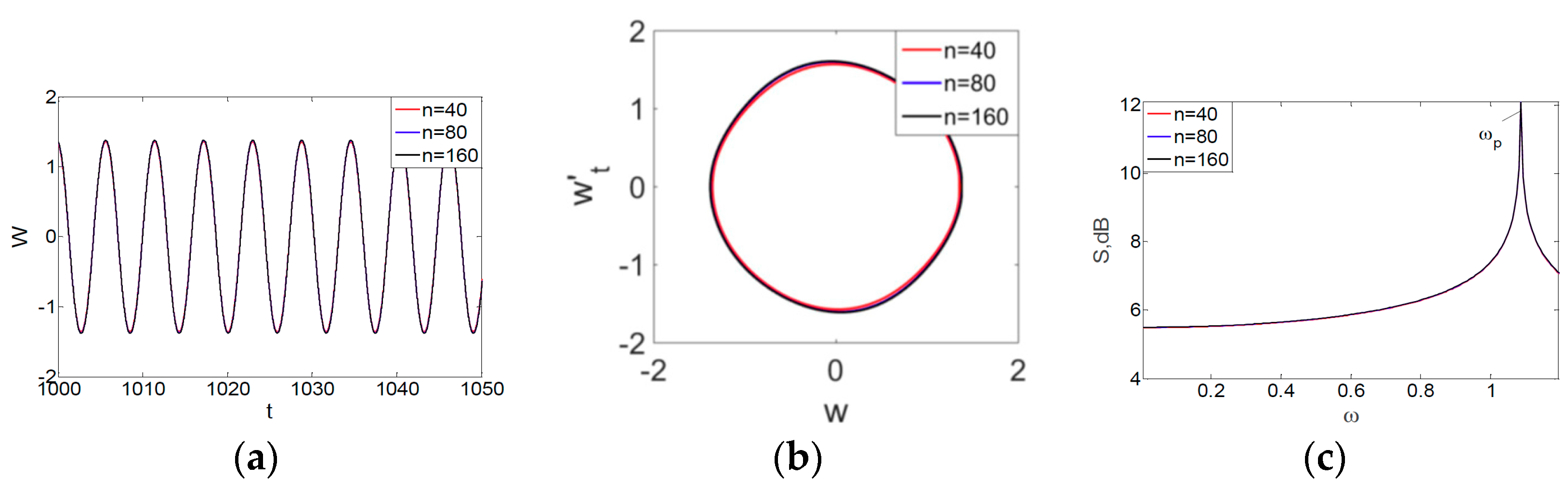
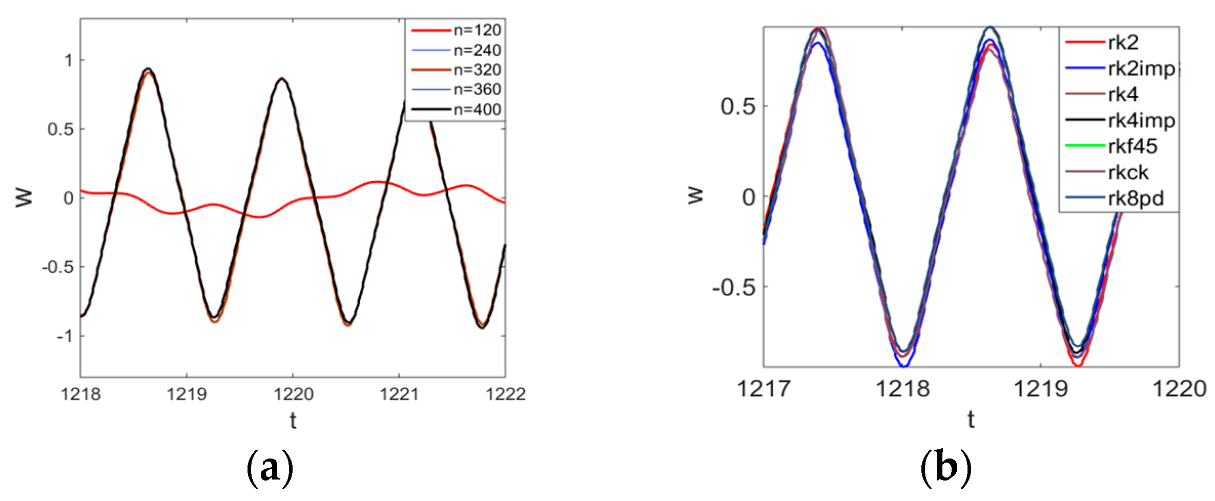
- Since PDEs are reduced to ODEs (Cauchy problem) using the FDM of second-order accuracy, their solution essentially depends on the number of beam length partitions (nodes). We need to find a number of partitions n, for which the solution coincided with the case of using n + 1 partitions. Furthermore, we want to achieve convergence even with respect to time history in the case of chaotic orbits. In monograph [30] dealing with a similar problem, the convergence was achieved only with respect to the periodic vibrations, and in the case of chaotic vibrations, only integral convergence was accepted, i.e., coincidence of power spectra was used to validate true chaos.
- The Cauchy problem was solved numerically and it is known that it depends on the chosen method and the integration step, which is why we chose different methods to validate the computational results: fourth order the Runge–Kutta method (RK4) and the second order Runge–Kutta method (RK2) [31], the fourth order Runge–Kutta–Fehlberg method (RKF45) [32,33], the fourth order Cash–Karp method (RKCK) [34], the eighth order Runge–Kutta–Prince–Dormand method (RK8PD) [35], the implicit second order Runge–Kutta method (rk2imp), and the fourth order Runge–Kutta implicit method (rk4imp). The implicit method makes it possible to include an arbitrary form of the used matrix of the related coefficients, whereas the RKF45, RKCK, and RK8PD methods allow for the automatic change of the computational step as well as to control errors introduced by integration.
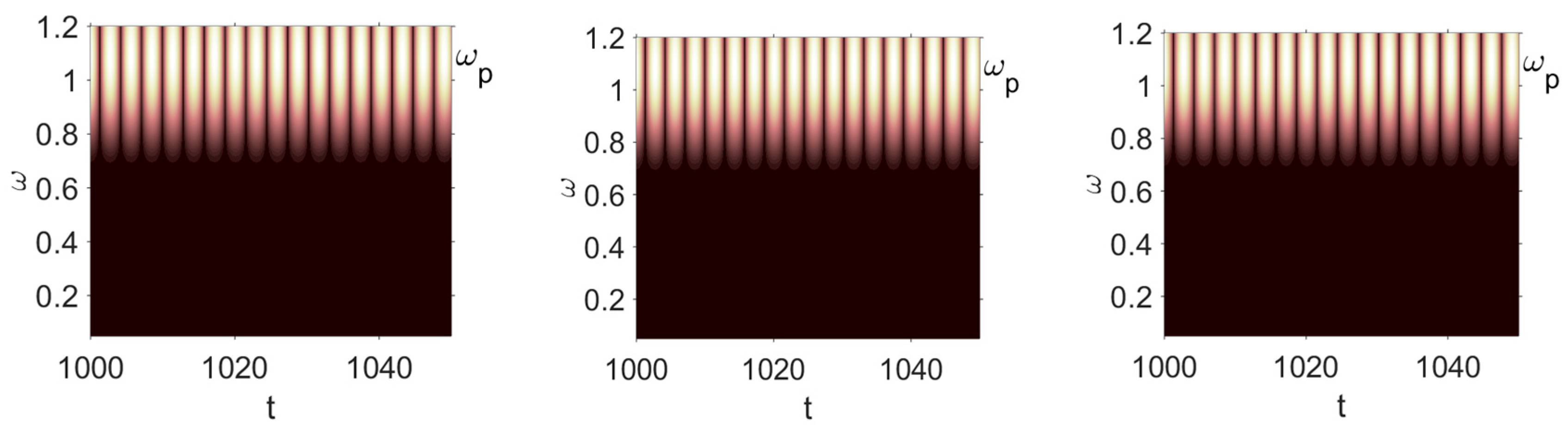
- For each of the introduced numbers of partitions of the beam length and the solutions to the Cauchy problems, the time histories (vibration signals), 2D and 3D phase portraits, the Fourier power spectra, the Morlet wavelets, snapshots of beam deflections, and Poincaré maps were constructed. For the chosen signal, a 2D wavelet spectrum was also constructed. The following mother wavelets were employed: Haar [36]; Shannon–Kotelnikov and Meyer [37]; Daubechies wavelets from db2 up to db16 [38]; coiflets, simlets, and the Morlet and complex Morlet wavelets [39]; and the wavelets based on the derivative of the Gauss function of the order higher than eight. However, the Haar and Shannon–Kotelnikov wavelets were unsuitable for our purpose. Namely, the first one was badly localized with respect to frequency, and the second one with respect to time.
- 4.
- Since we employed the Gulick [12] definition of chaos, we needed to compute and validate signs of the largest Lyapunov exponents (LLEs). Spectra of Lyapunov exponents were estimated based on the Kantz [42], Wolf [43] and Rosenstein [44] methods. The results were eventually accepted if they agreed to the fourth decimal place.
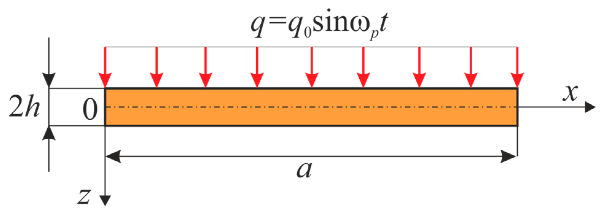
2. Problem Statement and the Mathematical Model
3. Methods of Solution
3.1. FDM Method
3.2. Lyapunov Exponents
3.3. Case Studies and Results Analysis
4. Concluding Remarks
- Convergence of the employed numerical methods was investigated with respect to the spatial and time coordinates (finite difference method with approximation O(h2) and the Runge–Kutta type methods). Numerical results showed that, to achieve reliable conclusions, it is necessary to conduct a complex analysis and, owing to the proposed methodology, each signal should be studied separately.
- The most negligible effect was observed when purple noise was added—beam vibrations remained periodic. On the other hand, beam vibrations were significantly influenced by pink noise. The degree of chaotization of the system essentially depends on the presence of low-frequency components in noise. The employment of the Morlet mother wavelets allowed to detect time evolution of frequencies during chaotic beam vibrations (Table 2 ()).
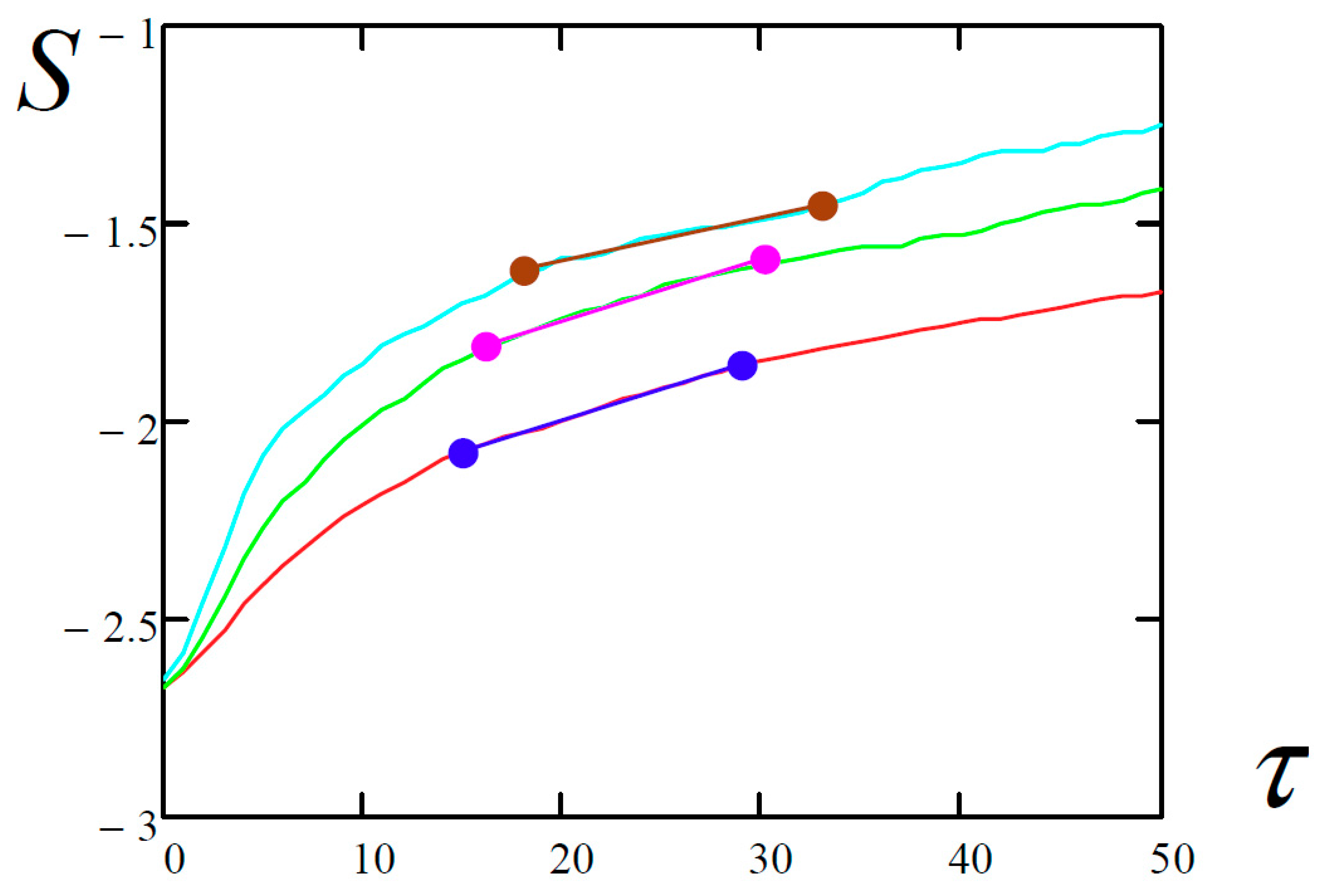
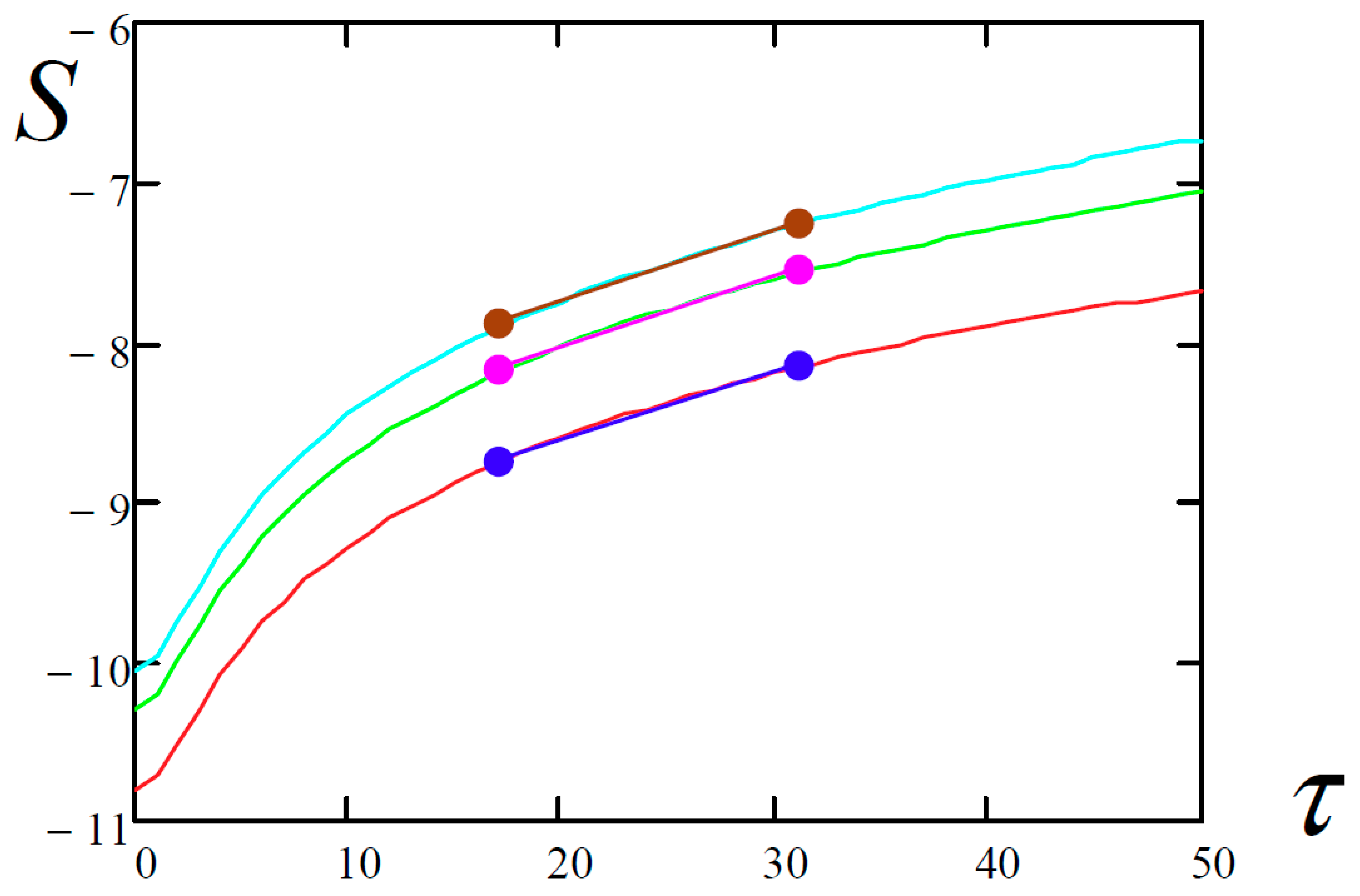
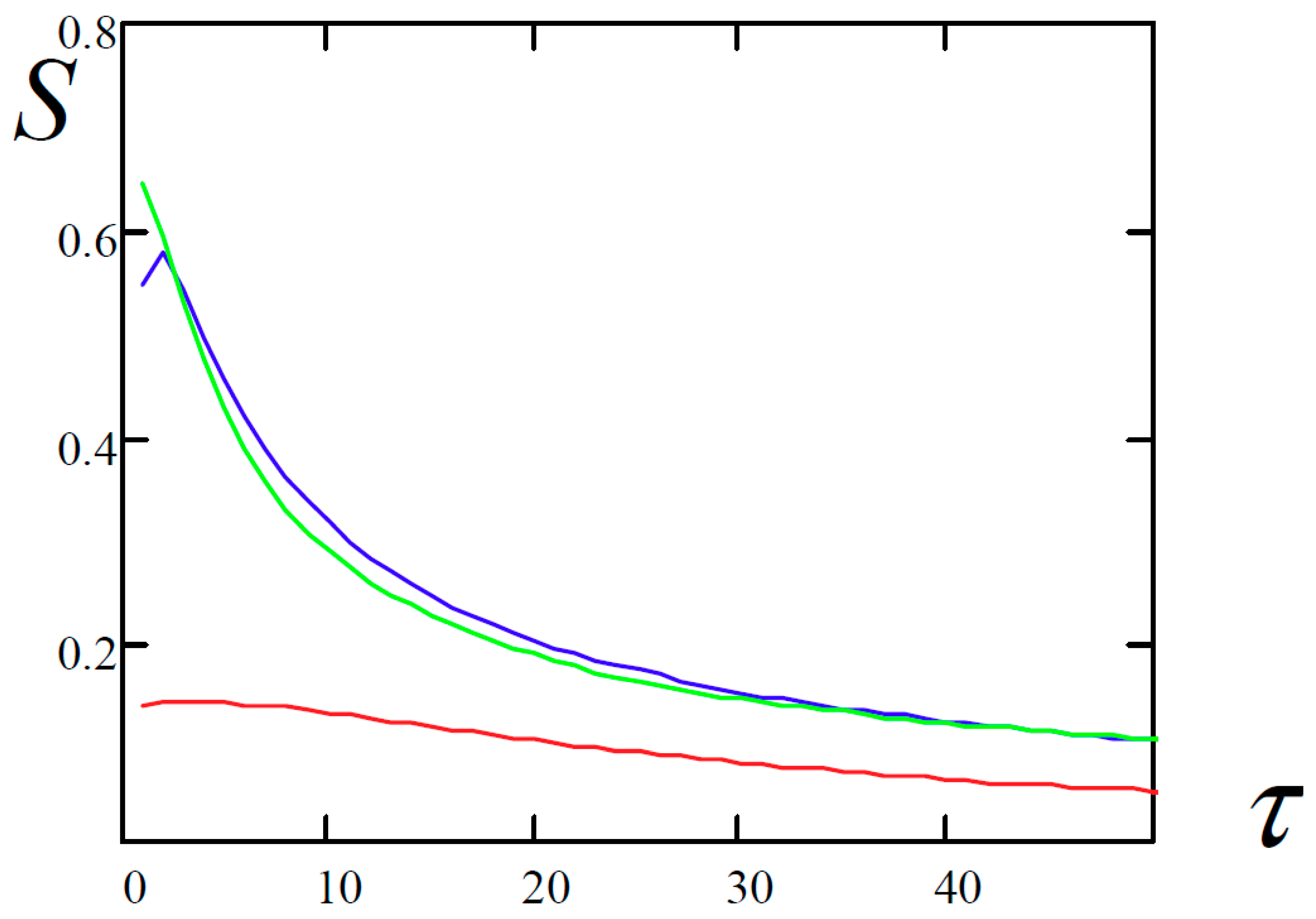
- It was found, illustrated and discussed that the Wolf (W), Kantz (K) and Rosenstein (R) methods may yield significantly different values of Lyapunov exponents for the same signal. On the other hand, all the above-mentioned methods exhibited good correlation when used to study different colored noises.
- The obtained results indicate a need to employ a more complex study by using qualitatively different numerical approaches to obtain reliable/true chaotic vibrations.
Acknowledgments
Author Contributions
Conflicts of Interest
References
- Ruelle, D.; Takens, F. On the nature of turbulence. Commun. Math Phys. 1971, 20, 167–192. [Google Scholar] [CrossRef]
- Berge, P.; Dubois, M.; Manneville, P.; Pomeau, Y. Intermittency in Rayleigh-Benard convection. J. Phys. Paris Lett. 1980, 41, L341–L345. [Google Scholar] [CrossRef]
- Horsthemke, W.; Lefever, R. Noise-Induced Transitions. Theory and Applications in Physics, Chemistry, and Biology; Springer: Berlin, Germany, 1984. [Google Scholar]
- Awrejcewicz, J.; Krysko, V.A.; Vakakis, A.F. Nonlinear Dynamics of Continuous Elastic System; Springer: Berlin, Germany, 2004. [Google Scholar]
- Awrejcewicz, J.; Krysko, A.V.; Bochkarev, V.V.; Babenkova, T.V.; Papkova, I.V.; Mrozowski, J. Chaotic vibrations of two-layered beams and plates with geometric, physical and design nonlinearities. Int. J. Bifurc. Chaos 2011, 21, 2837–2851. [Google Scholar] [CrossRef]
- Awrejcewicz, J.; Krysko, A.V.; Soldatov, V.; Krysko, V.A. Analysis of the nonlinear dynamics of the Timoshenko flexible beams using wavelets. J. Comput. Nonlinear Dyn. 2012, 7, 011005. [Google Scholar] [CrossRef]
- Awrejcewicz, J.; Krysko, V.A.; Papkova, I.V.; Krysko, A.V. Routes to chaos in continuous mechanical systems. Part 1: Mathematical models and solution methods. Chaos Solitons Fractals 2012, 45, 687–708. [Google Scholar] [CrossRef]
- Awrejcewicz, J.; Krysko, V.A.; Papkova, I.V.; Krysko, A.V. Routes to chaos in continuous mechanical systems. Part 2: Modeling transitions from regular to chaotic dynamics. Chaos Solitons Fractals 2012, 45, 709–720. [Google Scholar] [CrossRef]
- Awrejcewicz, J.; Krysko, V.A.; Papkova, I.V.; Krysko, A.V. Routes to chaos in continuous mechanical systems. Part 3: The Lyapunov exponents, hyper, hyper-hyper and spatial-temporal chaos. Chaos Solitons Fractals 2012, 45, 721–736. [Google Scholar] [CrossRef]
- Amabili, M. Nonlinear vibrations of doubly curved shallow shells. Int. J. Non Linear Mech. 2005, 40, 683–710. [Google Scholar] [CrossRef]
- Amabili, M.; Sarkar, A.; Païdoussis, M.P. Chaotic vibrations of circular cylindrical shells: Galerkin versus reduced-order models via the proper orthogonal decomposition method. J. Sound Vib. 2006, 290, 736–762. [Google Scholar] [CrossRef]
- Gulick, D. Encounters with Chaos; McGraw-Hill: New York, NY, USA, 1992. [Google Scholar]
- Holmes, P.J. A nonlinear oscillator with a strange attractor. Philos. Trans. R. Soc. A 1979, 292, 419–448. [Google Scholar] [CrossRef]
- Yee, H.; Sweby, C. Dynamical approach study of spurious steady state numerical solutions of nonlinear differential equations. II. Global asymptotic behavior of time discretizations. Int. J. Comput. Fluid Dyn. 1995, 4, 219–283. [Google Scholar] [CrossRef]
- Corless, R.M.; Essex, C.; Nerenberg, M.A.H. Numerical methods can suppress chaos. Phys. Lett. A 1991, 157, 27–36. [Google Scholar] [CrossRef]
- Tseng, W.Y.; Dugundji, J. Nonlinear vibrations of a buckled beam under harmonic excitation. ASME J. Appl. Mech. 1971, 38, 467–476. [Google Scholar] [CrossRef]
- Moon, F.C.; Holmes, P.J. A magneto-elastic strange attractor. J. Sound Vib. 1979, 65, 275–296. [Google Scholar] [CrossRef]
- Holmes, P.J.; Marsden, J. A partial differential equation with infinitely many periodic orbits: Chaotic oscillations of a forced beam. Arch. Ration. Mech. Anal. 1981, 76, 135–166. [Google Scholar] [CrossRef]
- Szemplińska-Stupnicka, W.; Plaut, R.H.; Hsieh, J.C. Period doubling and chaos in unsymmetric structures under parametric excitation. ASME J. Appl. Mech. 1989, 56, 947–952. [Google Scholar] [CrossRef]
- Bar-Yoseph, P.Z.; Fisher, D.; Gottlieb, O. Spectral element methods for nonlinear spatio-temporal dynamics of an Euler-Bernoulli beam. Comput. Mech. 1996, 19, 136–151. [Google Scholar] [CrossRef]
- Dunne, J.F.; Ghanbari, M. Efficient extreme value prediction for nonlinear beam vibrations using measured random response histories. Nonlinear Dyn. 2001, 24, 71–101. [Google Scholar] [CrossRef]
- Ge, G.; Xu, J. Stochastic bifurcation of one flexible beam subject to axial Gauss white noise excitation. In Proceedings of the 4th IEEE Conference on Industrial Electronics and Applications, Xi’an, China, 25–27 May 2009; pp. 1647–1653. [Google Scholar]
- Cacciola, P.; Impollonia, N.; Muscolino, G. Crack detection and location in a damaged beam vibrating under white noise. Comput. Struct. 2003, 81, 1773–1782. [Google Scholar] [CrossRef]
- Sahoo, B.; Panda, L.N.; Pohit, G. Nonlinear dynamics of an Euler-Bernoulli beam with parametric and internal resonances. Procedia Eng. 2013, 64, 727–736. [Google Scholar] [CrossRef]
- Lan, C.B.; Qin, W.Y. Energy harvesting from coherent resonance of horizontal vibration of beam excited by vertical base motion. Appl. Phys. Lett. 2014, 105, 11391. [Google Scholar] [CrossRef]
- Xu, L.; Ma, Q. Existence of random attractors for the floating beam equation with strong damping and white noise. Bond. Value Probl. 2015, 2015, 126. [Google Scholar] [CrossRef]
- Devaney, R.L. An Introduction to Chaotic Dynamical Systems, 2nd ed.; Addison-Wesley: Reading, MA, USA, 1989. [Google Scholar]
- Banks, J.; Brooks, J.; Davis, G.; Stacey, P. On Devaney’s definition of chaos. Am. Math. Mon. 1992, 99, 332–334. [Google Scholar] [CrossRef]
- Knudsen, C. Chaos without periodicity. Am. Math. Mon. 1994, 101, 563–565. [Google Scholar] [CrossRef]
- Awrejcewicz, J.; Krysko, V.A.; Papkova, I.V.; Krysko, A.V. Deterministic Chaos in One-Dimentional Continuous Systems; World Scientific: Singapore, 2016. [Google Scholar]
- Süli, E.; Mayers, D. An Introduction to Numerical Analysis; Cambridge University Press: Cambridge, UK, 2003. [Google Scholar]
- Fehlberg, E. Low-Order Classical Runge-Kutta Formulas with Step Size Control and Their Application to Some Heat Transfer Problems; NASA Technical Report; NASA: Washington, WA, USA, 1969; p. 315.
- Fehlberg, E. Klassische Runge-Kutta-Formeln vierter und niedrigerer Ordnung mit Schrittweiten-Kontrolle und ihre Anwendung auf Wärmeleitungsprobleme. Computing 1970, 6, 61–71. [Google Scholar] [CrossRef]
- Cash, J.R.; Karp, A.N. A variable order Runge-Kutta method for initial value problems with rapidly varying right-hand sides. ACM Trans. Math. Softw. 1990, 16, 201–222. [Google Scholar] [CrossRef]
- Dormand, J.R.; Prince, P.J. A family of embedded Runge-Kutta formulae. J. Comput. Appl. Math. 1980, 6, 19–26. [Google Scholar] [CrossRef]
- Haar, A. Zur Theorie der orthogonalen Funktionensysteme. Math. Ann. 1910, 69, 331–371. [Google Scholar] [CrossRef]
- Meyer, Y. Ondelettes, Functions Splines et Analyses Graduees; Lectures Given at the University of Torino: Torino, Italy, 1986. [Google Scholar]
- Daubechies, I.; Grossmann, А.; Meyer, Y. Painless nonorthogonal expansions. J. Math. Phys. 1986, 27, 1271–1283. [Google Scholar] [CrossRef]
- Grossman, A.; Morlet, S. Decomposition of Hardy functions into square separable wavelets of constant shape. SIAM J. Math. Anal. 1984, 15, 723–736. [Google Scholar] [CrossRef]
- Meyer, Y. Ondelettes et Fonctions Splines; Technical Report; Seminaire EDP; Ecole Polytechnigue: Paris, France, 1986. [Google Scholar]
- Meyer, Y. Wavelets: Algorithms and Applications; SIAM: Philadelphia, PA, USA, 1993. [Google Scholar]
- Kantz, H. A robust method to estimate the maximum Lyapunov exponent of a time series. Phys. Lett. A 1994, 185, 77–87. [Google Scholar] [CrossRef]
- Wolf, A.; Swift, J.B.; Swinney, H.L.; Vastano, J.A. Determining Lyapunov Exponents from a time series. Phys. D Nonlinear Phenom. 1985, 16, 285–317. [Google Scholar] [CrossRef]
- Rosenstein, M.T.; Collins, J.J.; De Luca, C.J. A Practical Method for Calculating Largest Lyapunov Exponents from Small Data Sets. Phys. D Nonlinear Phenom. 1993, 65, 117–134. [Google Scholar] [CrossRef]
- Volmir, A.S. Nonlinear Dynamics of Plates and Shells; Nauka: Moscow, Russian, 1972. [Google Scholar]

| Power Spectrum | Phase Portrait | Wavelet Spectrum | |
|---|---|---|---|
| N = 120 | 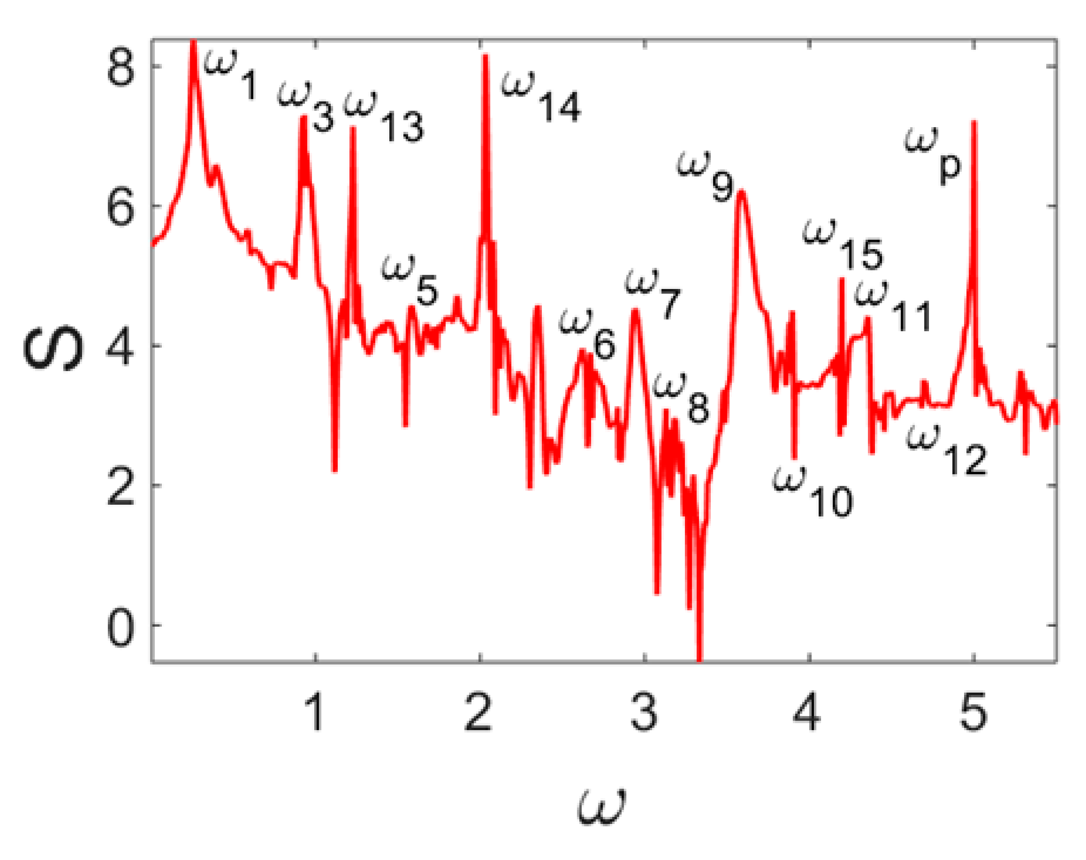 |  | 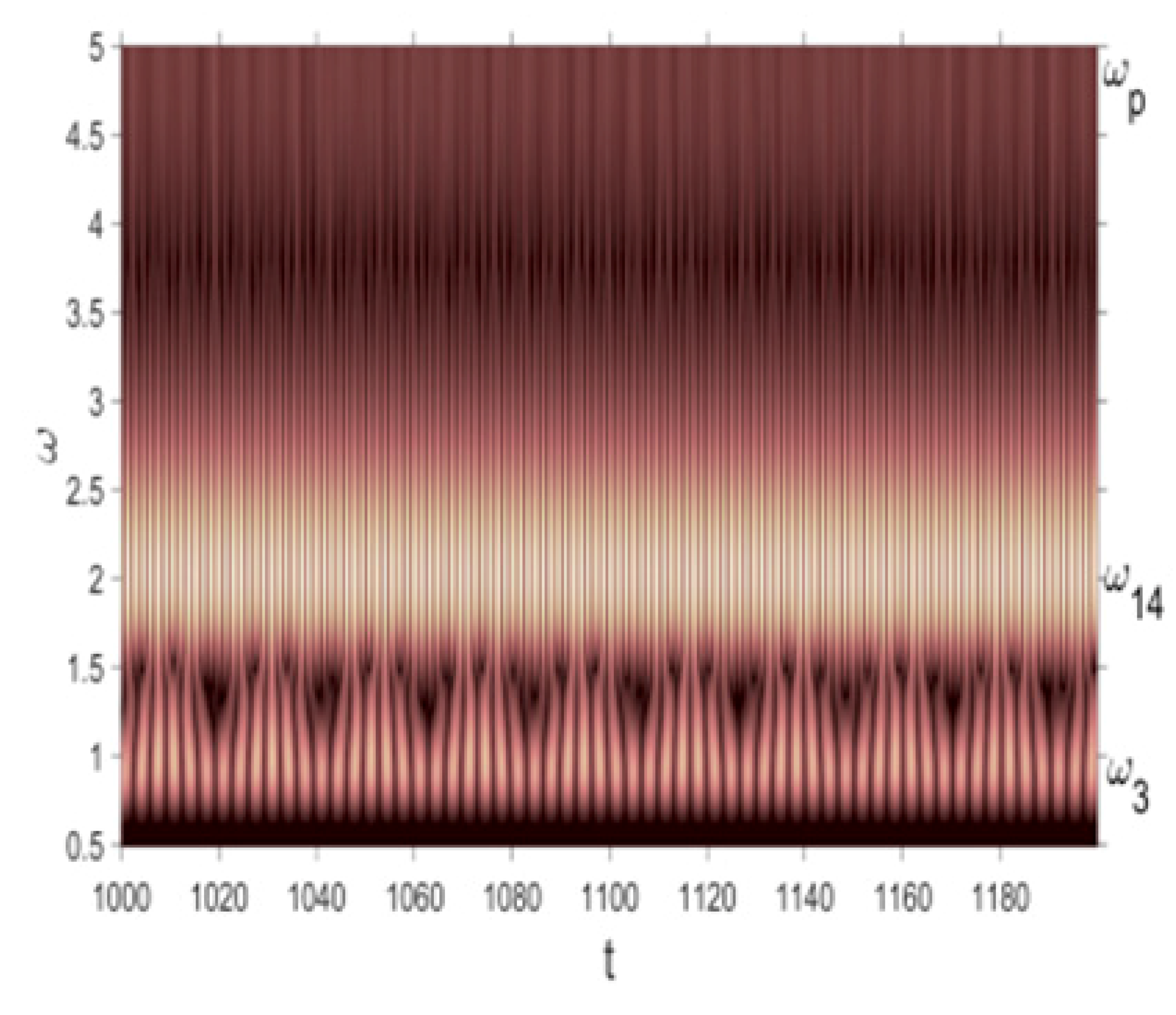 |
| N = 320 | 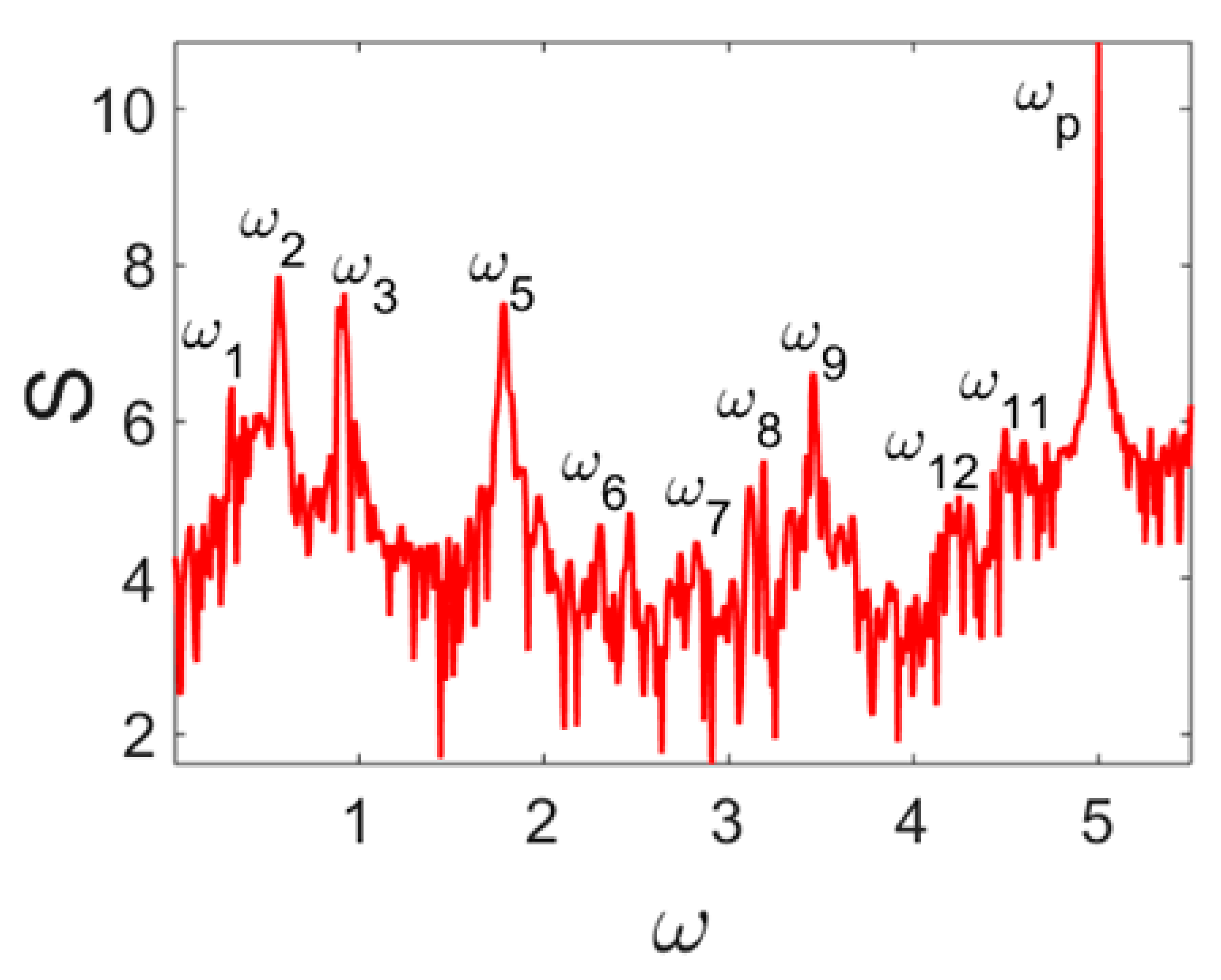 |  | 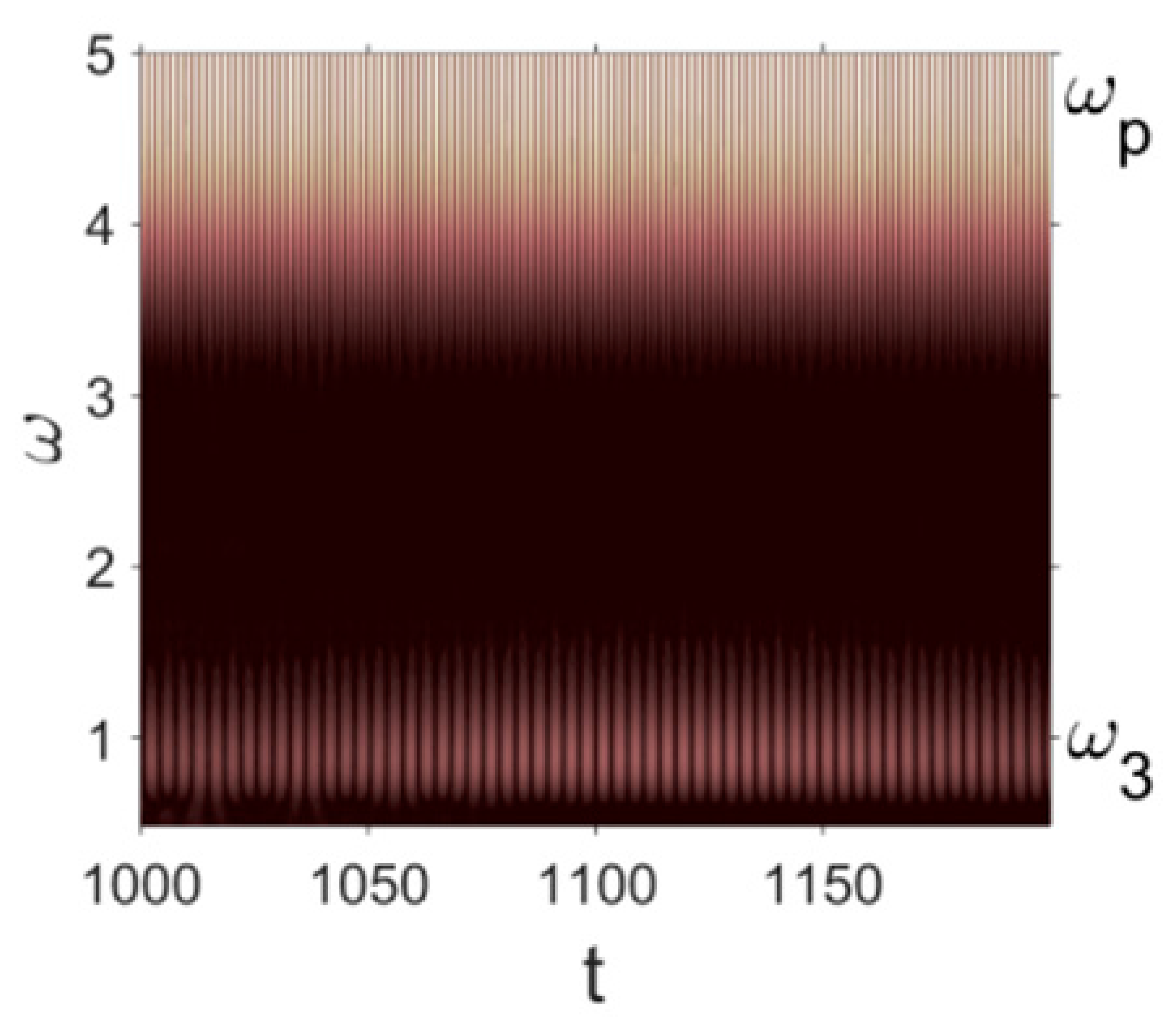 |
| N = 360, 400 | 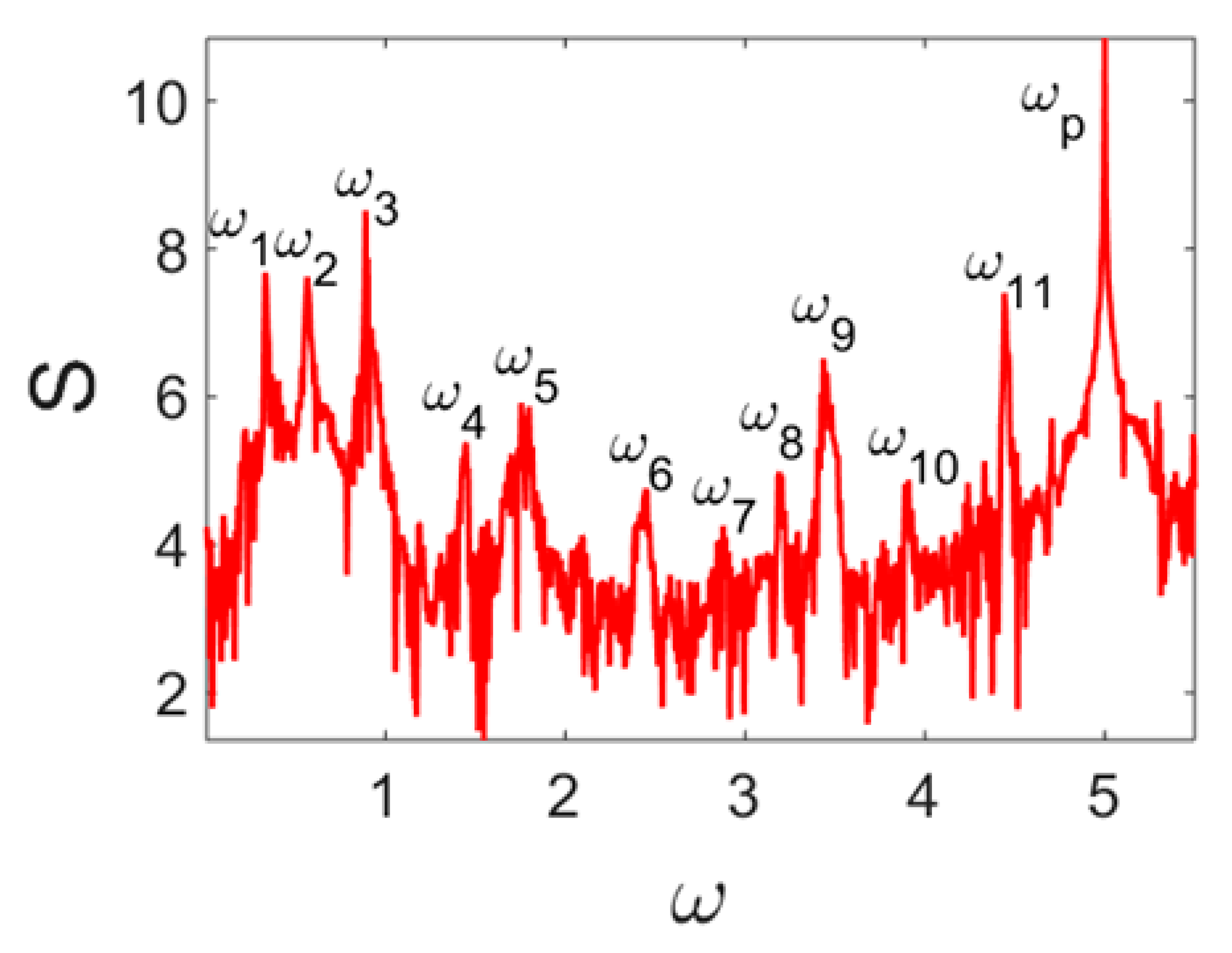 |  | 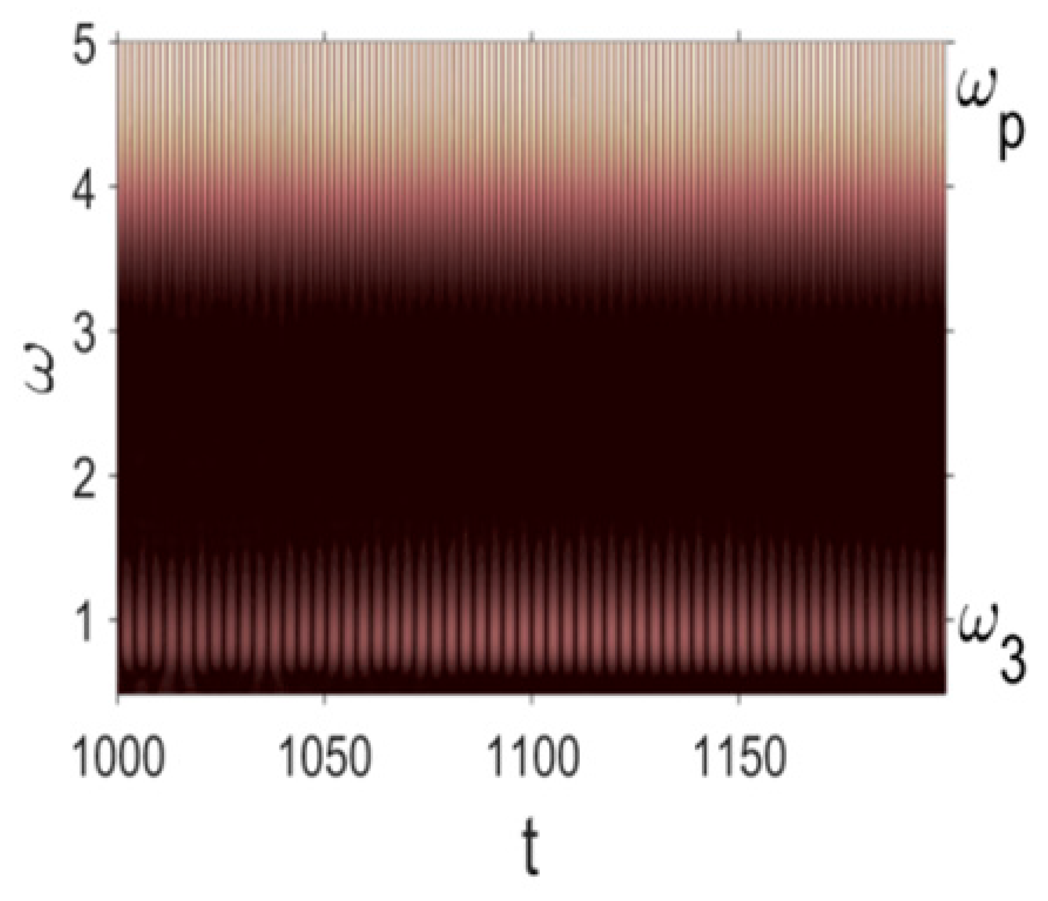 |
| λ | q | n | Wolf | Rosenstein | Kantz |
|---|---|---|---|---|---|
| 50 | 10000 | 160 | 0.10078 | 0.11334 | 0.04127 |
| 50 | 10000 | 200 | 0.07357 | 0.07359 | 0.02888 |
| 50 | 10000 | 240 | 0.09443 | 0.08599 | 0.03110 |
| 50 | 10000 | 360; 400 | 0.09885 | 0.07995 | 0.03190 |
| Noise | Morlet Wavelet | Fourier Spectrum | w(t) | 2D Phase Portrait | Poincaré Map |
|---|---|---|---|---|---|
purple | 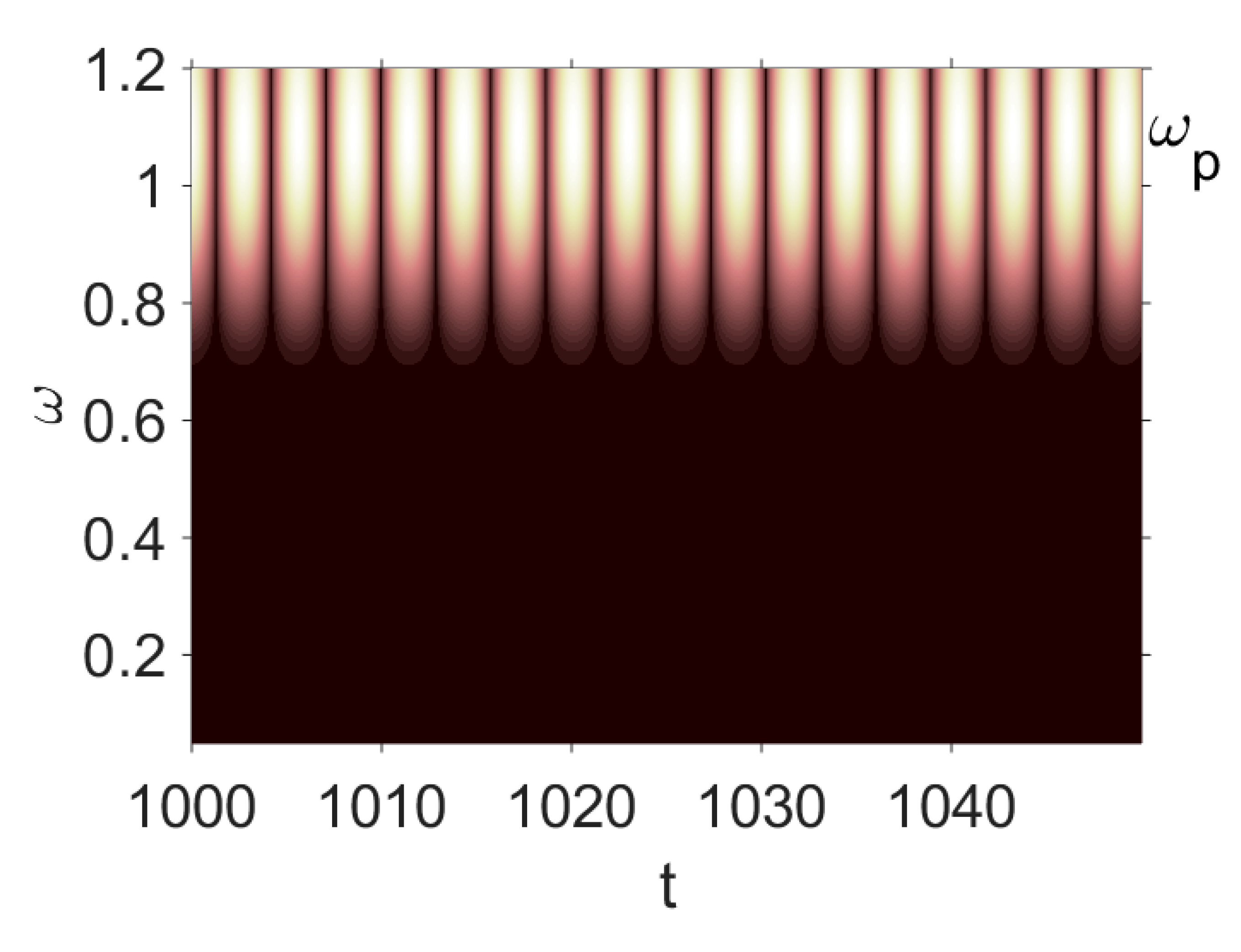 | 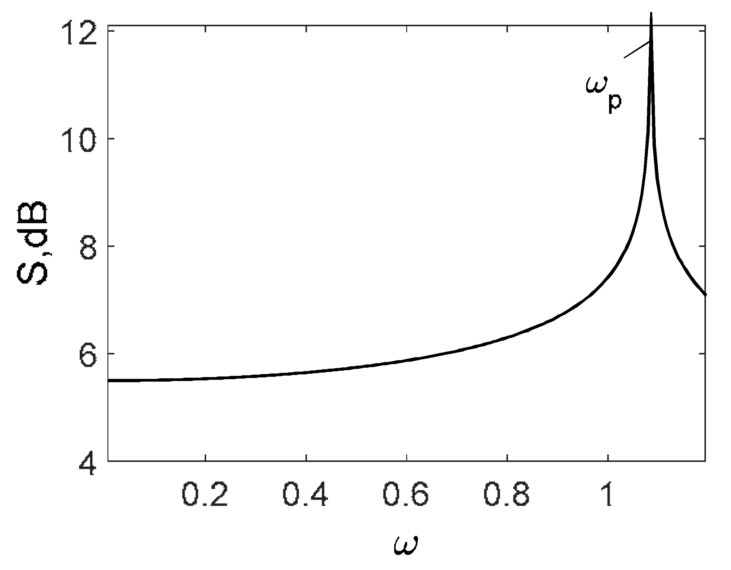 | 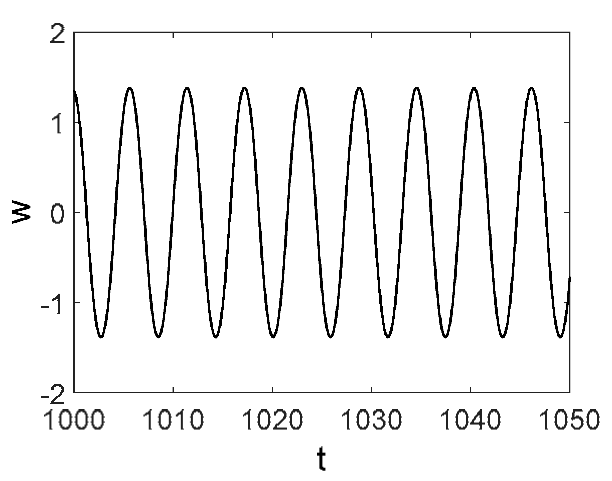 |  | 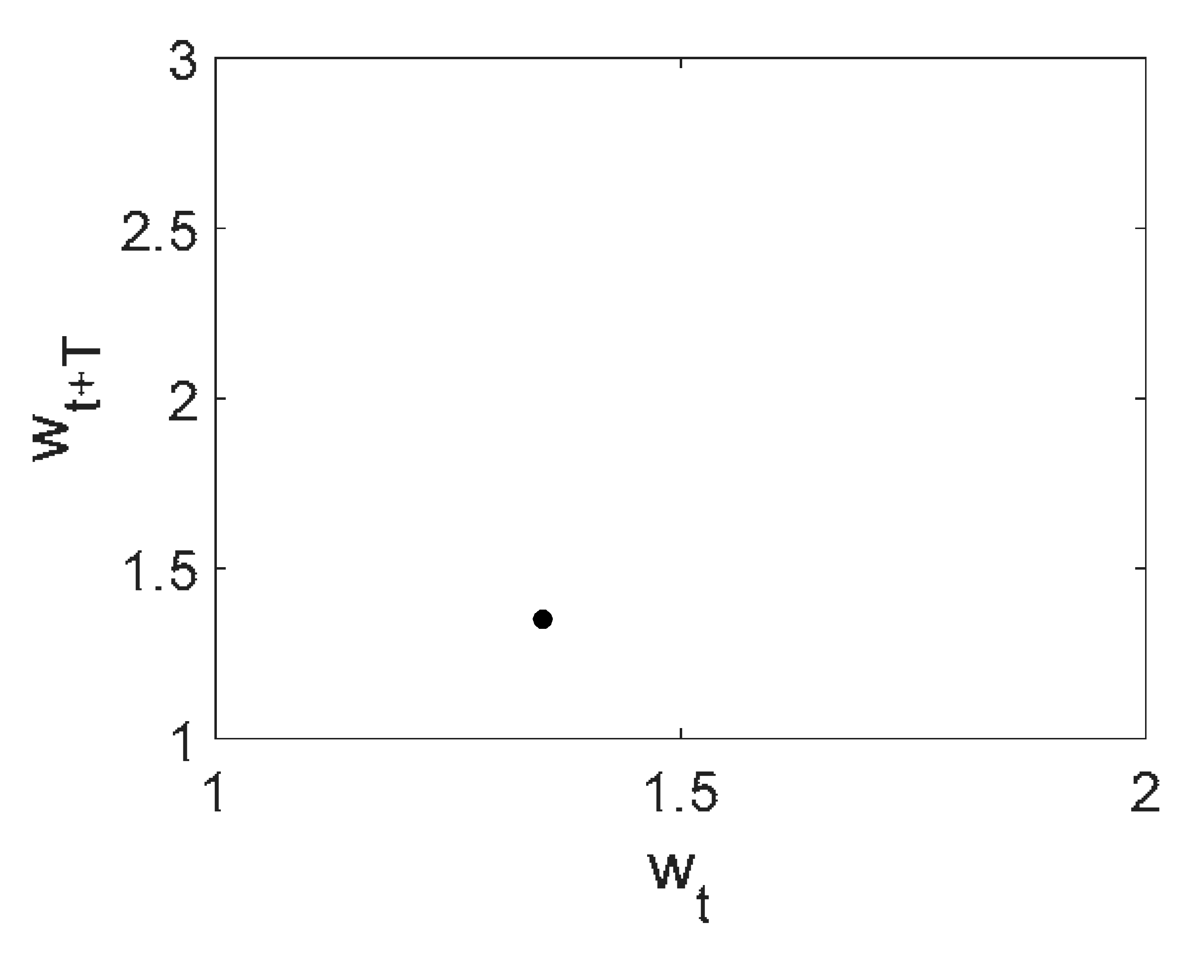 |
blue | 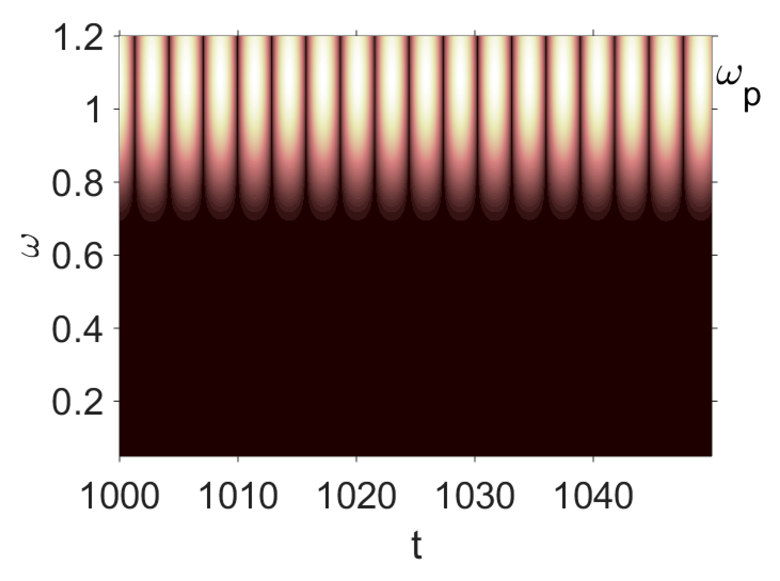 | 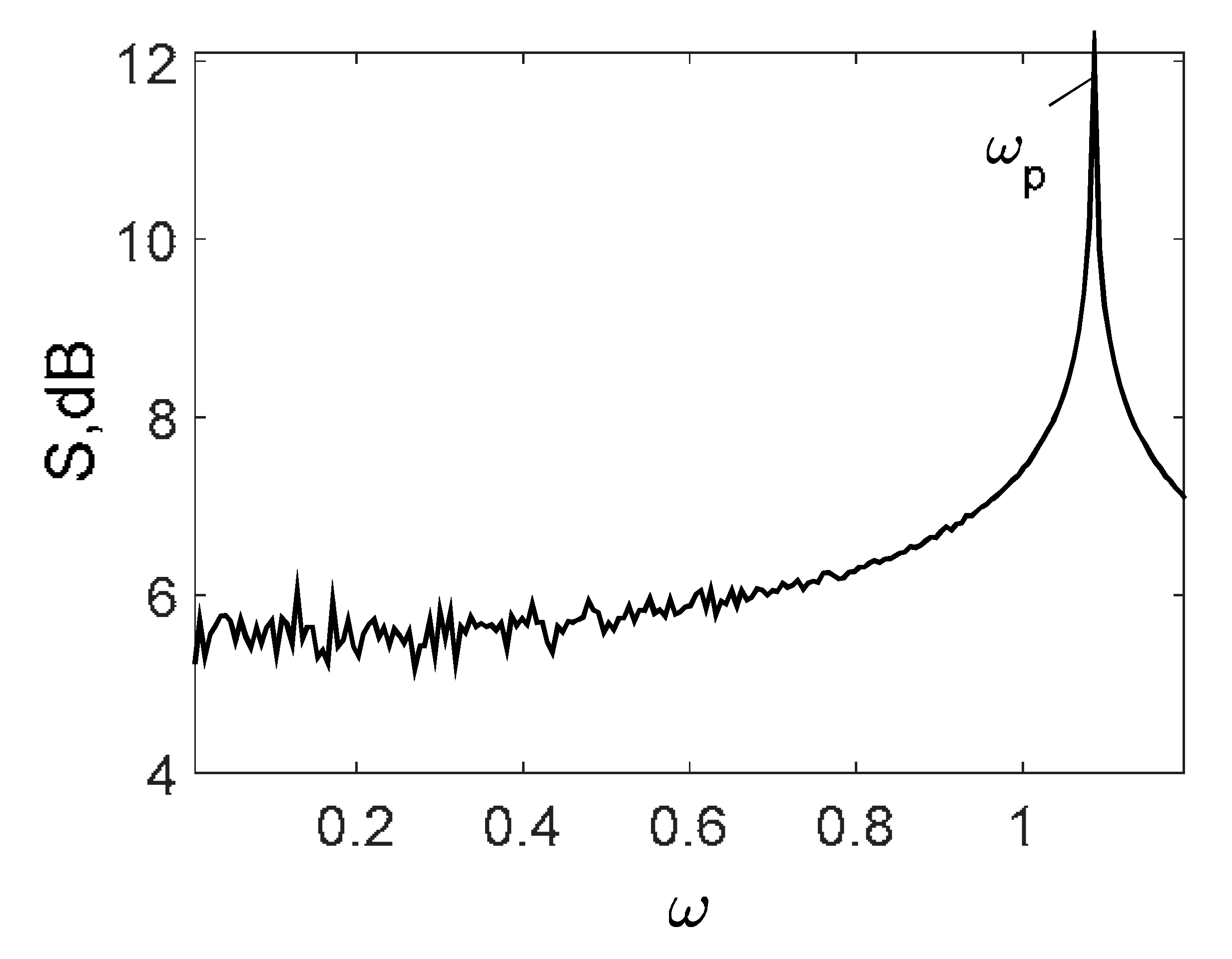 | 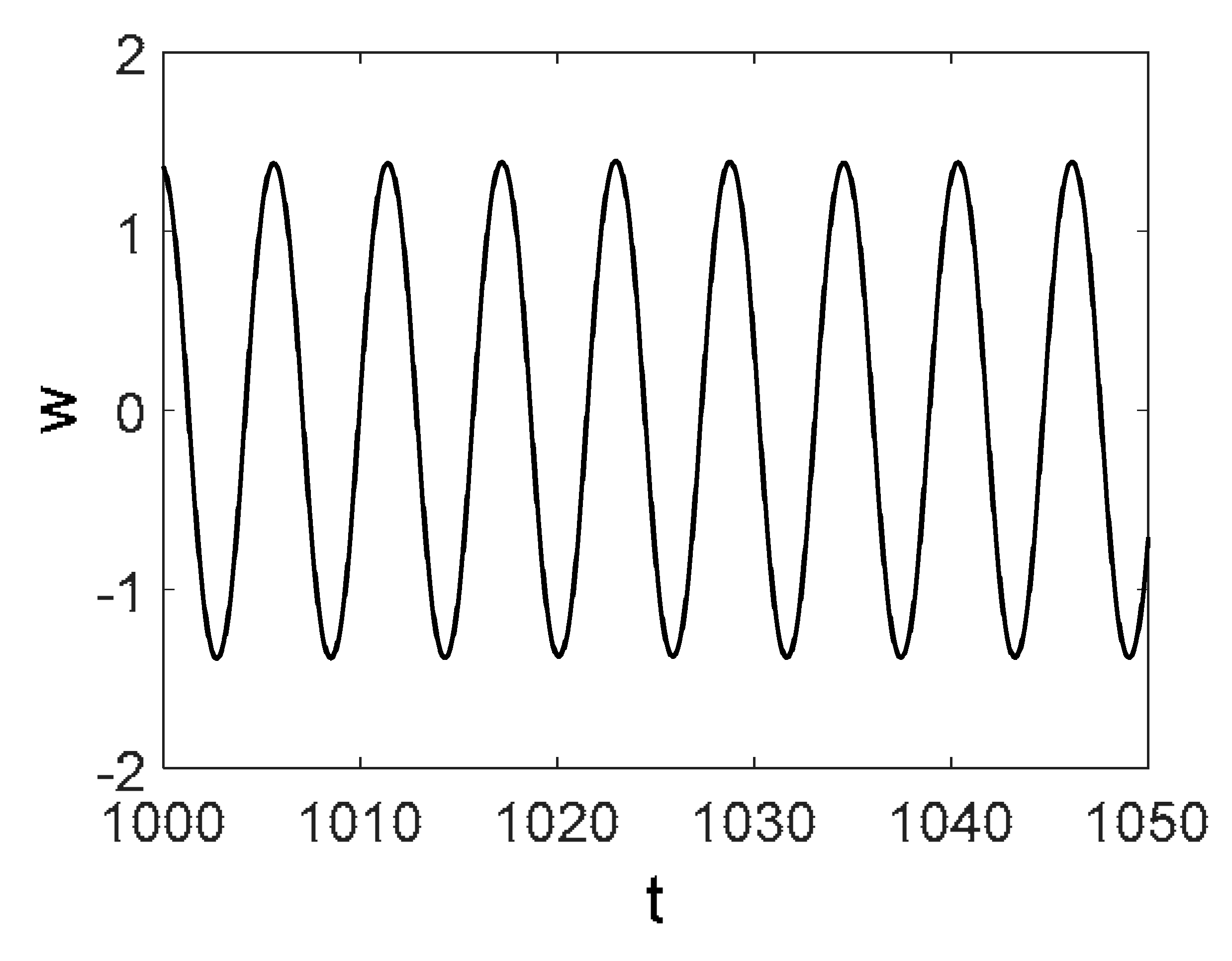 | 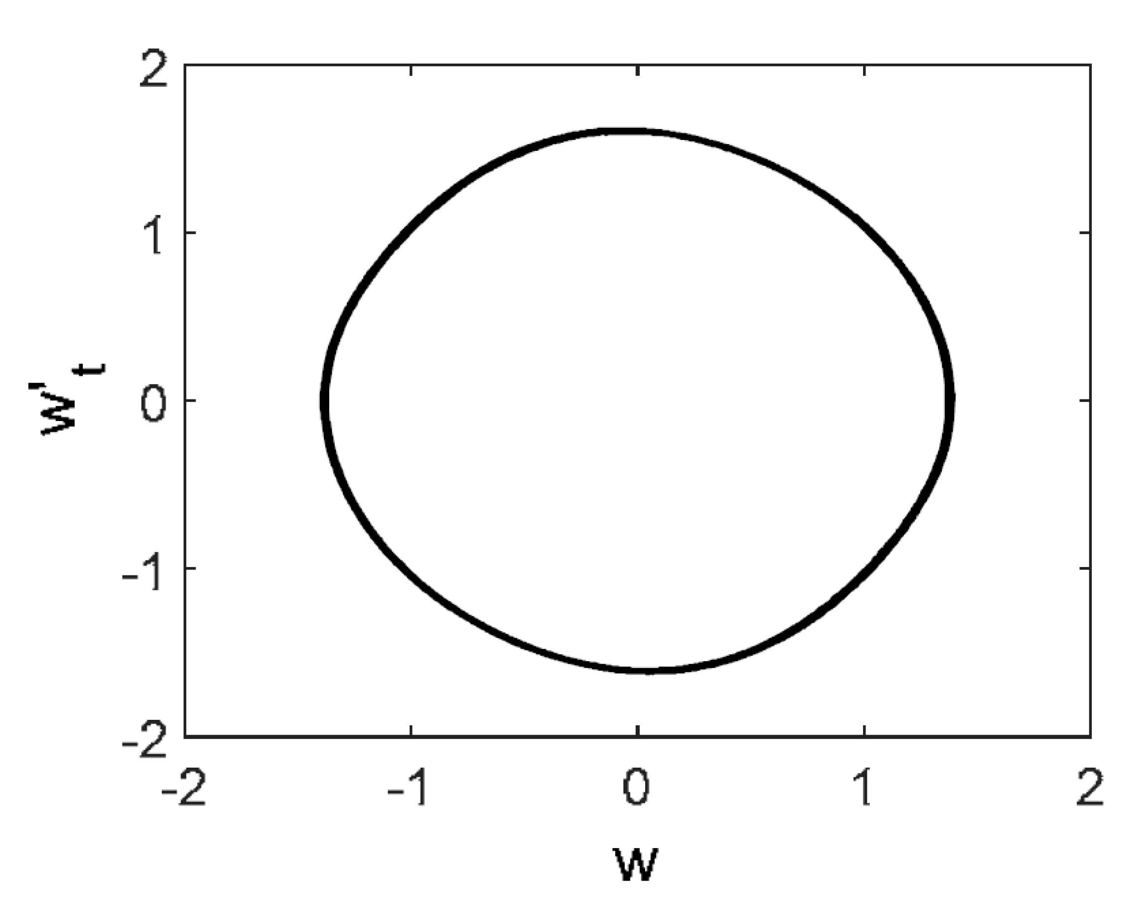 | 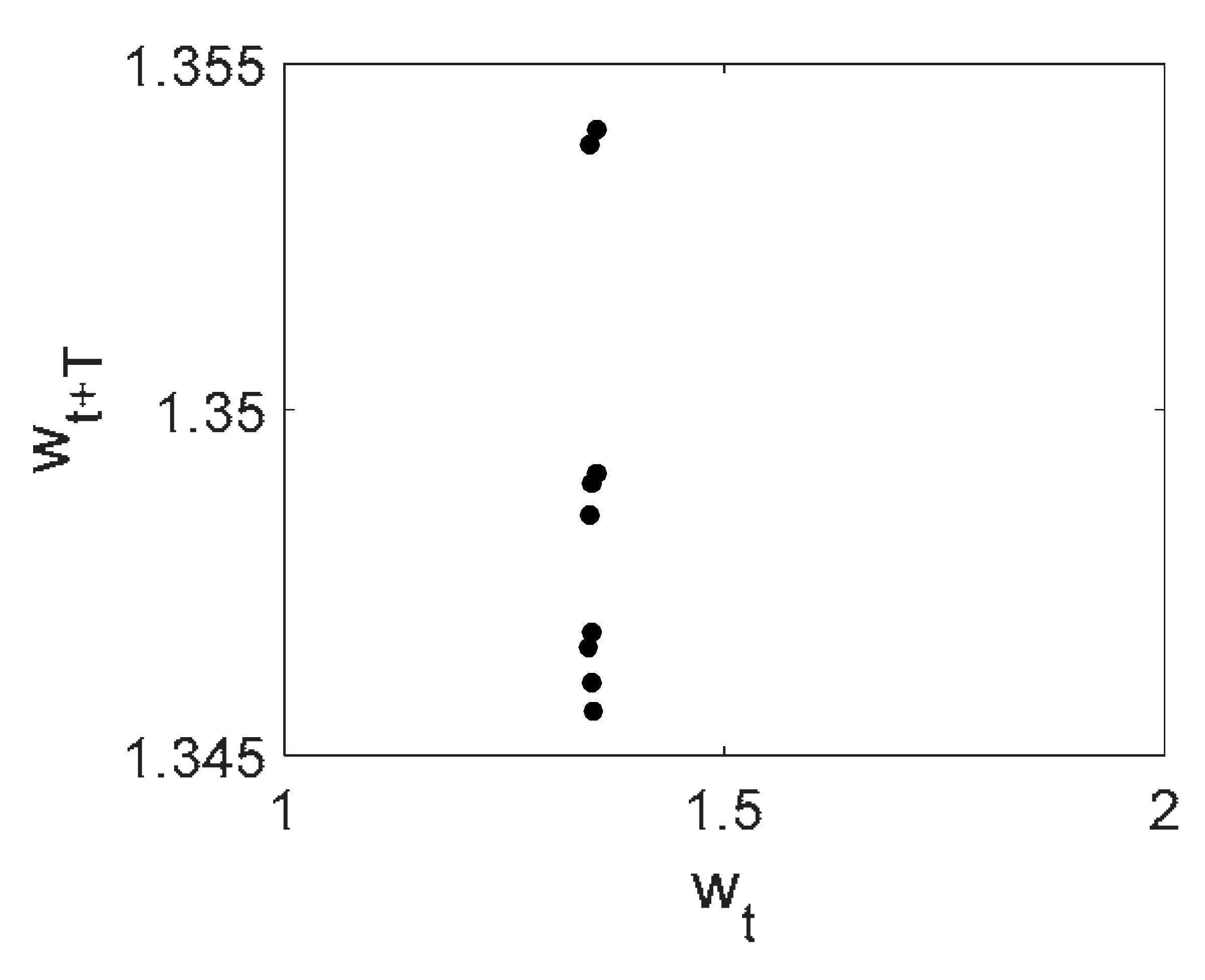 |
white | 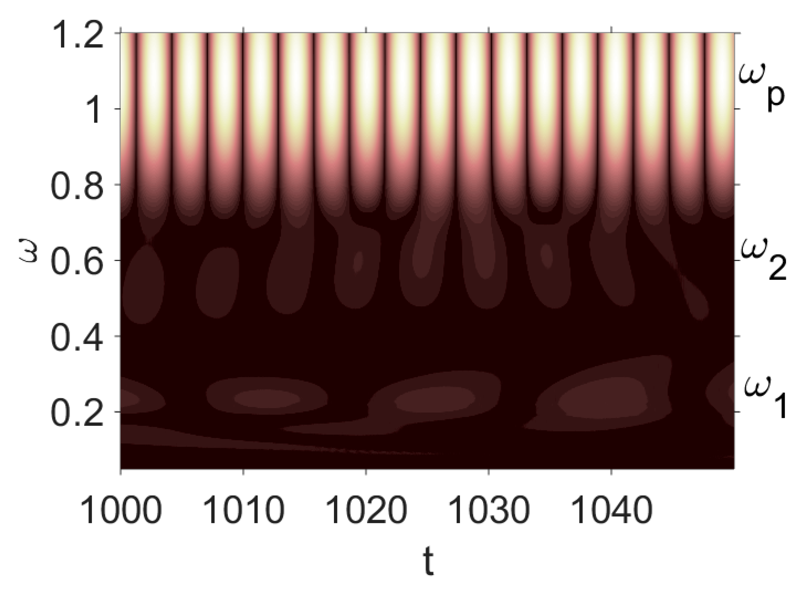 | 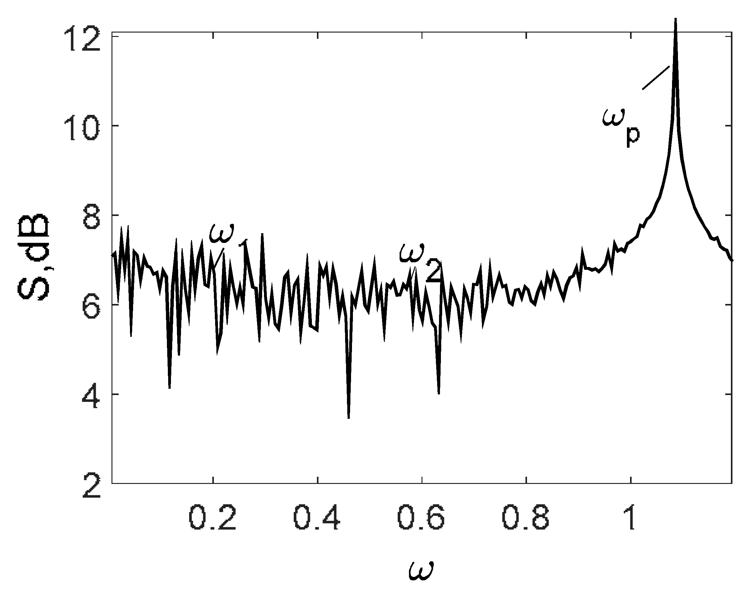 | 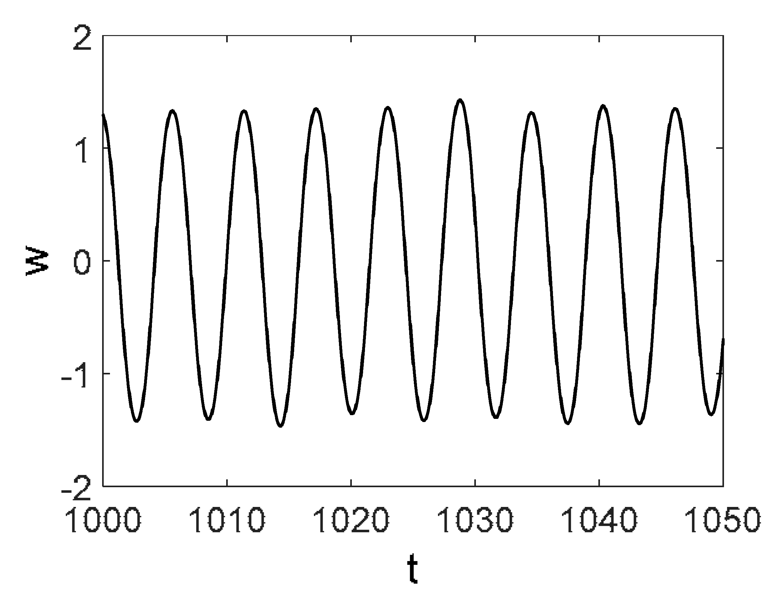 | 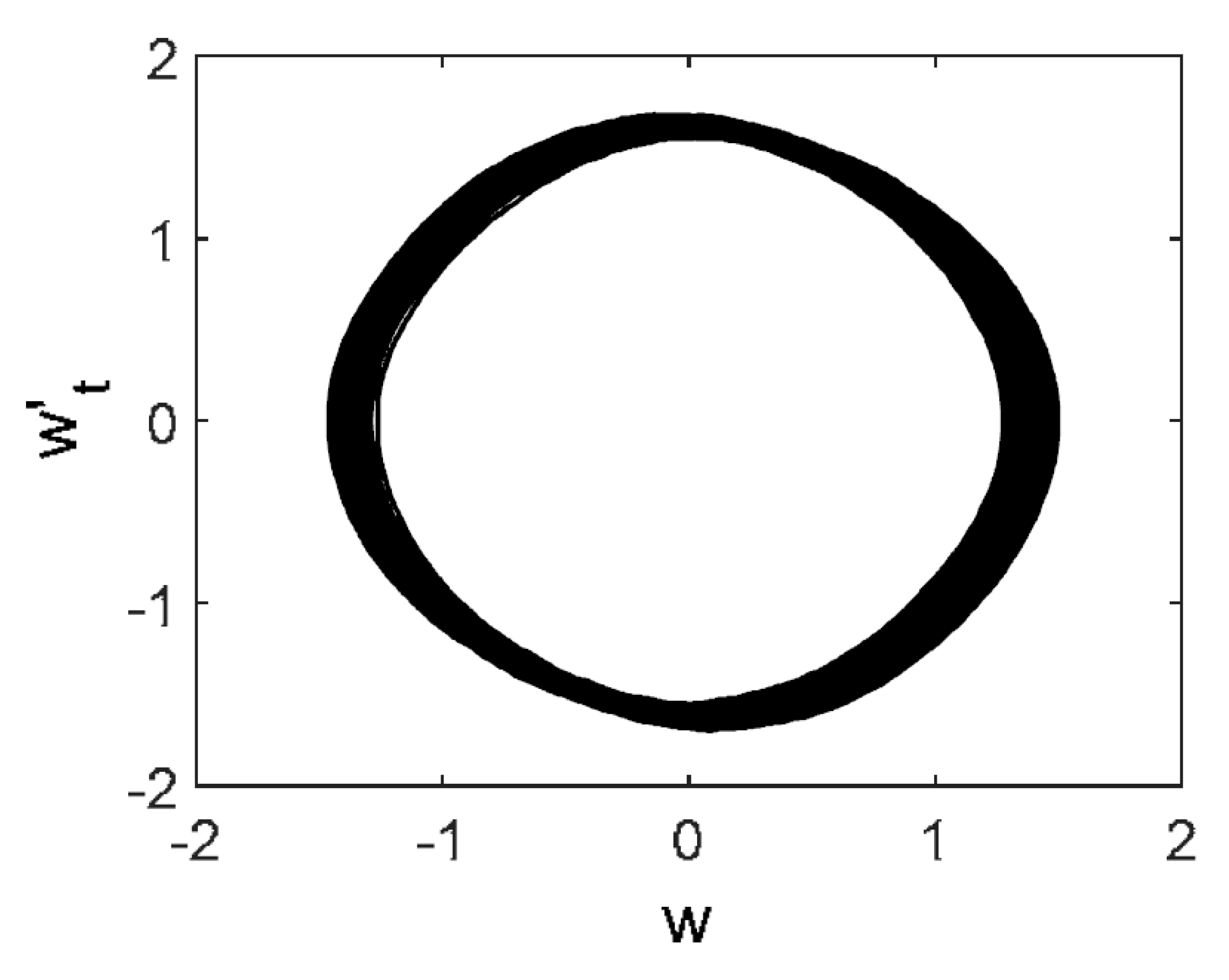 |  |
pink | 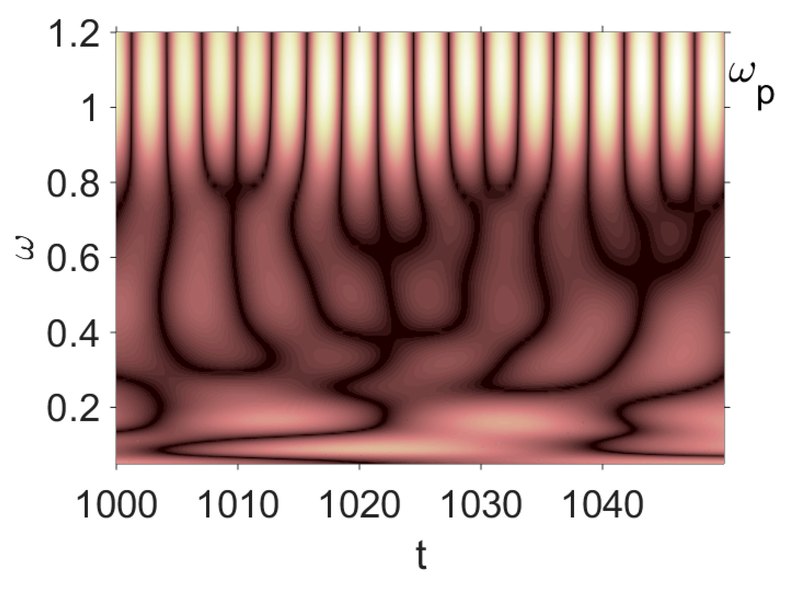 |  |  |  |  |
brown |  |  | 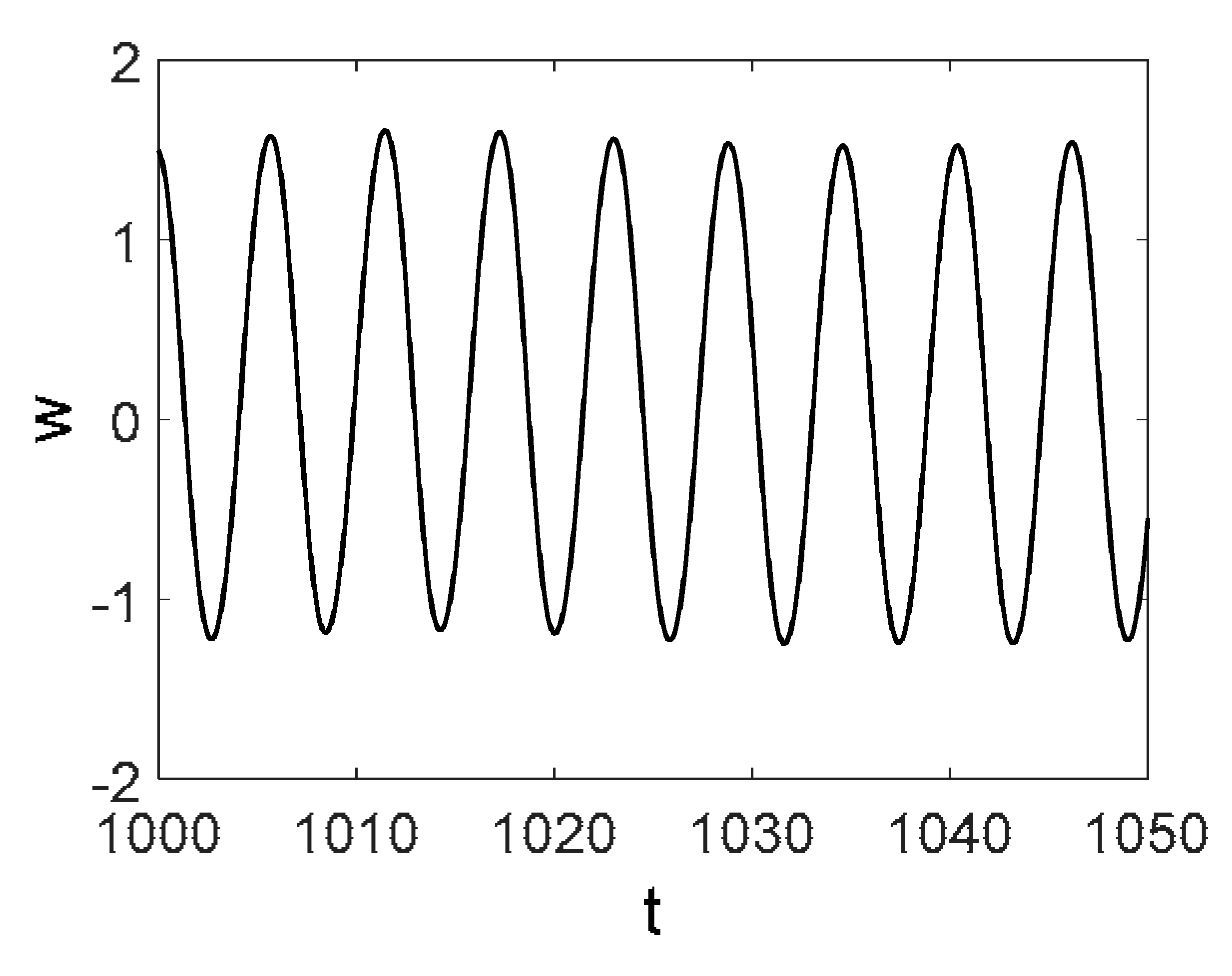 |  |  |
| Kantz | Rosenstein | Wolf |
|---|---|---|
 |  |  |
| W: 0.0 K: 0.0 R: 0.0 | W: 0.0 K: 210−2 R: 610−2 | W: 0.0 K: 310−2 R: 610−2 | W: 0.0 K: 310−2 R: 710−2 | W: 0.0 K: 210−2 R: 610−2 |
© 2018 by the authors. Licensee MDPI, Basel, Switzerland. This article is an open access article distributed under the terms and conditions of the Creative Commons Attribution (CC BY) license (http://creativecommons.org/licenses/by/4.0/).
Share and Cite
Awrejcewicz, J.; Krysko, A.V.; Erofeev, N.P.; Dobriyan, V.; Barulina, M.A.; Krysko, V.A. Quantifying Chaos by Various Computational Methods. Part 2: Vibrations of the Bernoulli–Euler Beam Subjected to Periodic and Colored Noise. Entropy 2018, 20, 170. https://doi.org/10.3390/e20030170
Awrejcewicz J, Krysko AV, Erofeev NP, Dobriyan V, Barulina MA, Krysko VA. Quantifying Chaos by Various Computational Methods. Part 2: Vibrations of the Bernoulli–Euler Beam Subjected to Periodic and Colored Noise. Entropy. 2018; 20(3):170. https://doi.org/10.3390/e20030170
Chicago/Turabian StyleAwrejcewicz, Jan, Anton V. Krysko, Nikolay P. Erofeev, Vitalyi Dobriyan, Marina A. Barulina, and Vadim A. Krysko. 2018. "Quantifying Chaos by Various Computational Methods. Part 2: Vibrations of the Bernoulli–Euler Beam Subjected to Periodic and Colored Noise" Entropy 20, no. 3: 170. https://doi.org/10.3390/e20030170
APA StyleAwrejcewicz, J., Krysko, A. V., Erofeev, N. P., Dobriyan, V., Barulina, M. A., & Krysko, V. A. (2018). Quantifying Chaos by Various Computational Methods. Part 2: Vibrations of the Bernoulli–Euler Beam Subjected to Periodic and Colored Noise. Entropy, 20(3), 170. https://doi.org/10.3390/e20030170