Model Error, Information Barriers, State Estimation and Prediction in Complex Multiscale Systems

Abstract
:| 1 Introduction | 3 |
| 2 Information Theory and Information Barriers with Model Error and Some Instructive Stochastic Models | 5 |
| 2.1 An Information-Theoretic Framework of Quantifying Model Error and Model Sensitivity | 5 |
| 2.2 Information Barriers in Capturing Model Fidelity . . . . . . . . . . . . . . . . . . . . . . | 7 |
| 2.2.1 First Information Barrier: Using Gaussian Approximation in Non-Gaussian Models | 8 |
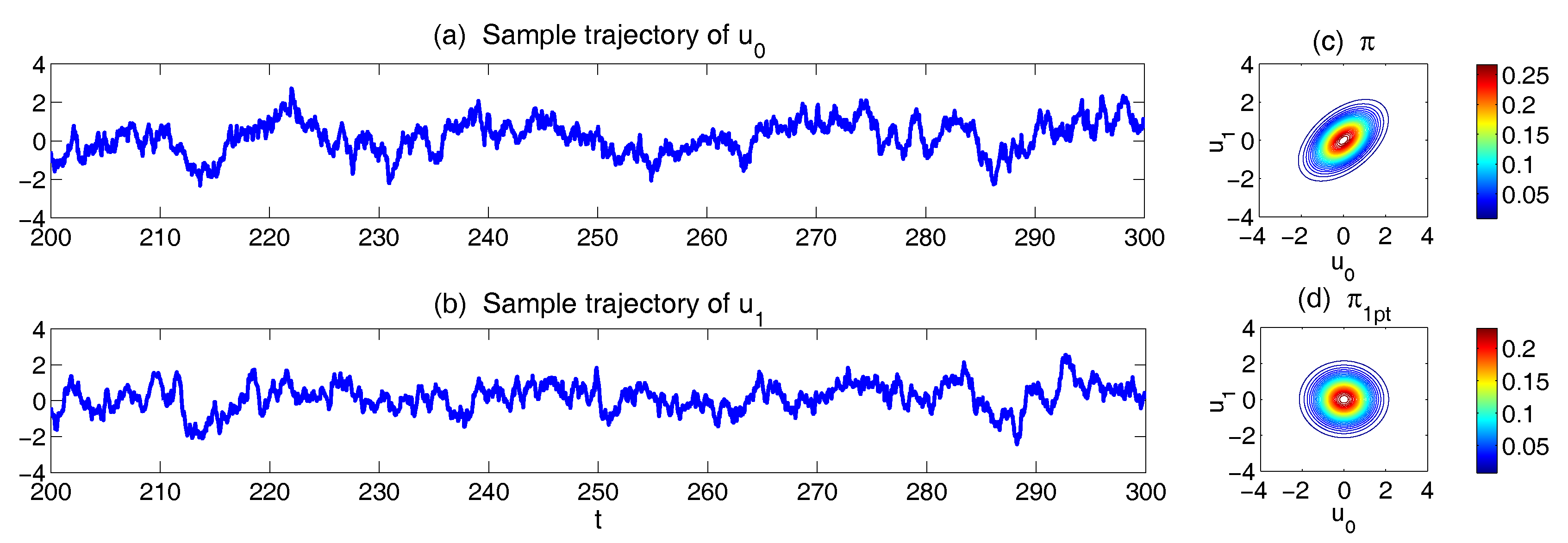
| 2.2.2 Second Information Barrier: Using Single Point Correlation to Approximate Full CorrelationMatrix . . . . . . . . . . . . . . . . . . . . . . . . . . . . . . . . . . . . . | 13 |
| 2.3 Intrinsic Information Barrier in Predicting Mean Response to the Change of Forcing . . | 15 |
| 2.4 Slow-Fast System and Reduced Model . . . . . . . . . . . . . . . . . . . . . . . . . . . . . | 17 |
| 2.5 Fitting Autocorrelation Function of Time Series by a Spectral Information Criteria . . . . | 19 |
| 3 Quantifying Model Error with Information Theory in State Estimation and Prediction | 23 |
| 3.1 Kalman Filter, State Estimation and Linear Stochastic Model Prediction . . . . . . . . . . | 23 |
| 3.2 Asymptotic Behavior of Prediction and Filtering in One-Dimensional Linear Stochastic | |
| Models withModel Error . . . . . . . . . . . . . . . . . . . . . . . . . . . . . . . . . . . . . | 26 |
| 3.2.1 Prediction . . . . . . . . . . . . . . . . . . . . . . . . . . . . . . . . . . . . . . . . . | 26 |
| 3.2.2 Filtering . . . . . . . . . . . . . . . . . . . . . . . . . . . . . . . . . . . . . . . . . . | 27 |
| 3.2.3 Comparison . . . . . . . . . . . . . . . . . . . . . . . . . . . . . . . . . . . . . . . . | 27 |
| 3.3 An Information Theoretical Framework for State Estimation and Prediction . . . . . . . | 28 |
| 3.3.1 Motivation Examples . . . . . . . . . . . . . . . . . . . . . . . . . . . . . . . . . . . | 28 |
| 3.3.2 Assessing the Skill of Estimation and Prediction Using Information Theory . . . | 30 |
| 3.4 State Estimation and Prediction for Complex Scalar Forced Ornstein–Uhlenbeck (OU) | |
| Processes . . . . . . . . . . . . . . . . . . . . . . . . . . . . . . . . . . . . . . . . . . . . . . | 31 |
| 3.5 State Estimation and Prediction for Multiscale Slow-Fast Systems . . . . . . . . . . . . . | 36 |
| 3.5.1 A 3 × 3 Linear Coupled Multiscale Slow-Fast System . . . . . . . . . . . . . . . . | 37 |
| 3.5.2 ShallowWater Flows . . . . . . . . . . . . . . . . . . . . . . . . . . . . . . . . . . . | 43 |
| 4 Information, Sensitivity and Linear Statistical Response—Fluctuation–Dissipation Theorem (FDT) | 47 |
| 4.1 Fluctuation–Dissipation Theorem (FDT) . . . . . . . . . . . . . . . . . . . . . . . . . . . . | 48 |
| 4.1.1 The General Framework . . . . . . . . . . . . . . . . . . . . . . . . . . . . . . . . . | 48 |
| 4.1.2 Approximate FDT Methods . . . . . . . . . . . . . . . . . . . . . . . . . . . . . . . | 49 |
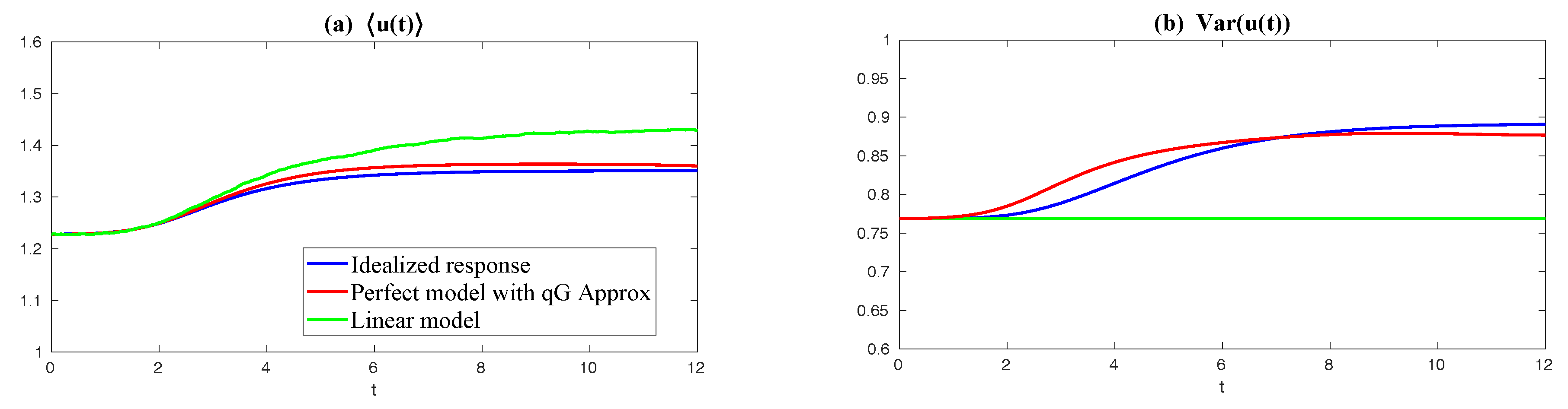
| 4.2 Information Barrier for Linear Reduced Models in Capturing the Response in the Second Order Statistics . . . . . . . . . . . . . . . . . . . . . . . . . . . . . . . . . . . . . . . . . . | 50 |
| 4.3 Information Theory for Finding the Most Sensitive Change Directions . . . . . . . . . . | 54 |
| 5 Given Time Series, Using Information Theory for Physics-Constrained Nonlinear Stochastic Model for Prediction | 59 |
| 5.1 A General Framework . . . . . . . . . . . . . . . . . . . . . . . . . . . . . . . . . . . . . . | 59 |
| 5.2 Model Calibration via Information Theory . . . . . . . . . . . . . . . . . . . . . . . . . . | 60 |
| 5.3 Applications: Assessing the Predictability Limits of Time Series Associated with Tropical Intraseasonal Variability . . . . . . . . . . . . . . . . . . . . . . . . . . . . . . . . . . . . . | 61 |
| 6 Reduced-Order Models (ROMs) for Complex Turbulent Dynamical Systems | 63 |
| 6.1 Strategies for Reduced-Order Models for Predicting the Statistical Responses and UQ . | 63 |
| 6.1.1 Turbulent Dynamical System with Energy-Conserving Quadratic Nonlinearity . | 63 |
| 6.1.2 Modeling the Effect of Nonlinear Fluxes . . . . . . . . . . . . . . . . . . . . . . . . | 65 |
| 6.1.3 A Reduced-Order Statistical Energy Model with Optimal Consistency and Sensitivity . . . . . . . . . . . . . . . . . . . . . . . . . . . . . . . . . . . . . . . . | 66 |
| 6.1.4 Calibration Strategy . . . . . . . . . . . . . . . . . . . . . . . . . . . . . . . . . . . | 67 |
| 6.2 Physics-Tuned Linear Regression Models for Hidden (Latent) Variables . . . . . . . . . . | 68 |
| 6.3 Predicting Passive Tracer Extreme Events . . . . . . . . . . . . . . . . . . . . . . . . . . . | 71 |
| 6.3.1 Approximating Nonlinear Advection Flow Using Physics-Tuned Linear Regression Model . . . . . . . . . . . . . . . . . . . . . . . . . . . . . . . . . . . . . | 73 |
| 6.3.2 Predicting Passive Tracer Extreme Events with Low-Order Stochastic Models . . | 76 |
| 7 Conclusions | 82 |
| A Derivations of Fisher Information from Relative Entropy | 83 |
| B Details of the Canonical Model for Low Frequency Atmospheric Variability | 84 |
| C Augmented System for Prediction and Filtering Distributions | 85 |
| C.1 Augmented System for Prediction . . . . . . . . . . . . . . . . . . . . . . . . . . . . . . . | 85 |
| C.2 Augmented System for Filtering . . . . . . . . . . . . . . . . . . . . . . . . . . . . . . . . | 86 |
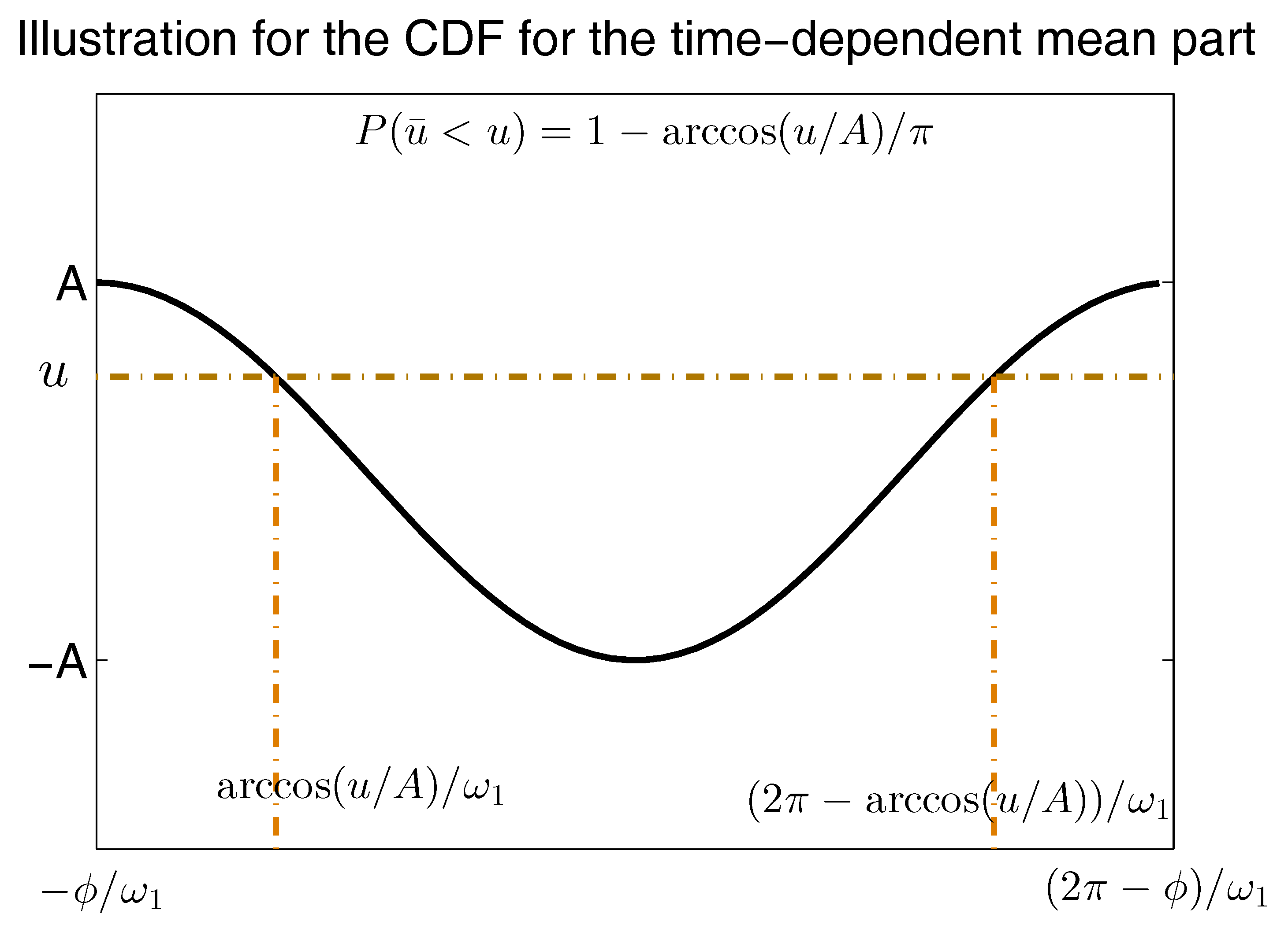
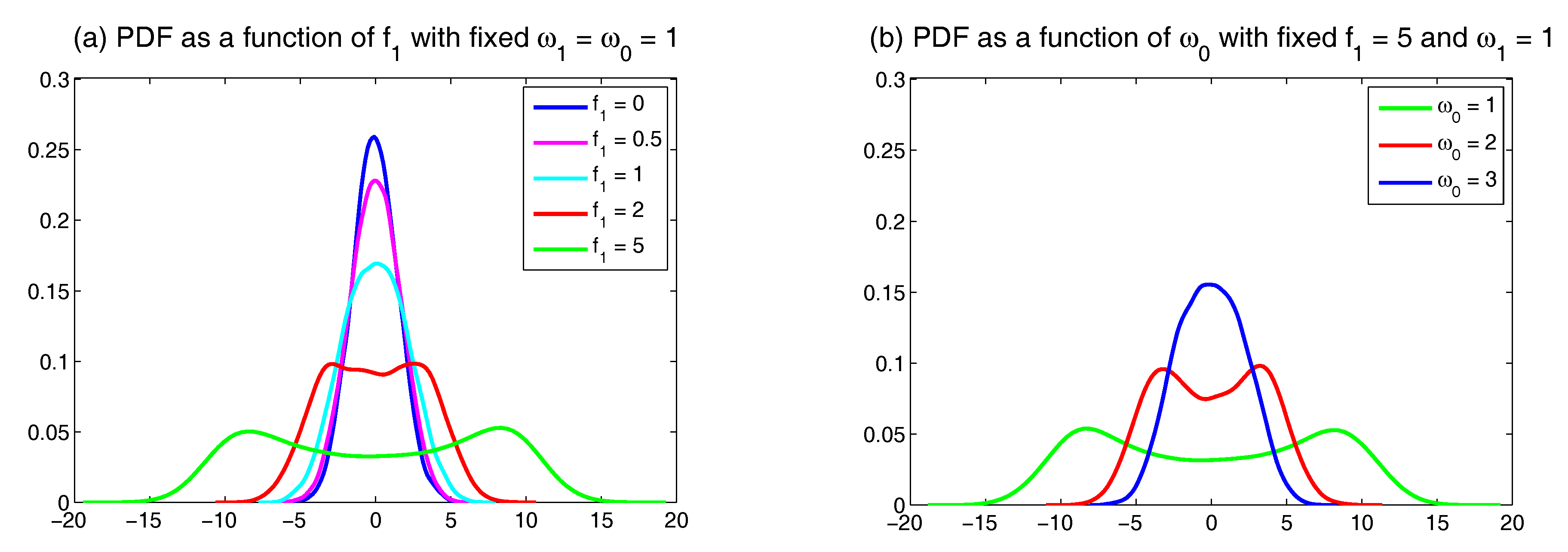
| D Possible Non-Gaussian PDFs of a Linear Model with Time-Periodic Forcing Based on the Sample Points in a Single Trajectory | 87 |
| References | 91 |
1. Introduction
- How to measure the skill (i.e., the statistical accuracy) of a given imperfect model in reproducing the present states and predicting the future states in an unbiased fashion?
- How to make the best possible estimate of model sensitivity to changes in external or internal parameters by utilizing the imperfect knowledge available of the present state? What are the most sensitive parameters for the change of the model status given uncertain knowledge of the present state?
- How to design cheap and practical reduced models that are nevertheless able to capture both the main statistical features of nature and the correct response to external/internal perturbations?
- How to develop a systematic data-driven nonlinear modeling and prediction framework that provides skillful forecasts and allows accurate quantifications of the forecast uncertainty?
- How to build effective models, efficient algorithms and unbiased quantification criteria for online data assimilation (state estimation or filtering) and prediction especially in the presence of model error?
2. Information Theory and Information Barriers with Model Error and Some Instructive Stochastic Models
2.1. An Information-Theoretic Framework of Quantifying Model Error and Model Sensitivity
2.2. Information Barriers in Capturing Model Fidelity
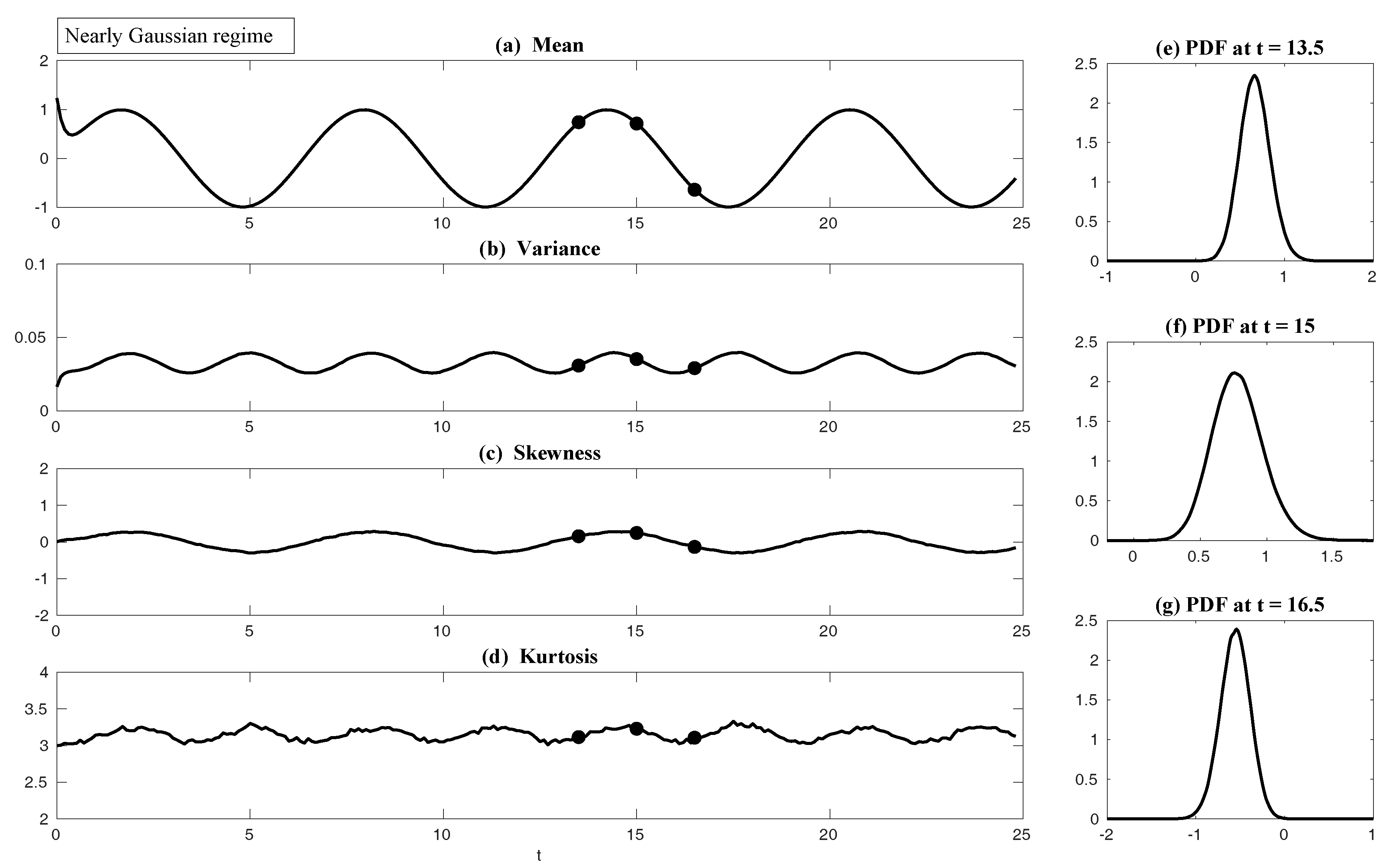
2.2.1. First Information Barrier: Using Gaussian Approximation in Non-Gaussian Models
2.2.2. Second Information Barrier: Using Single Point Correlation to Approximate Full Correlation Matrix
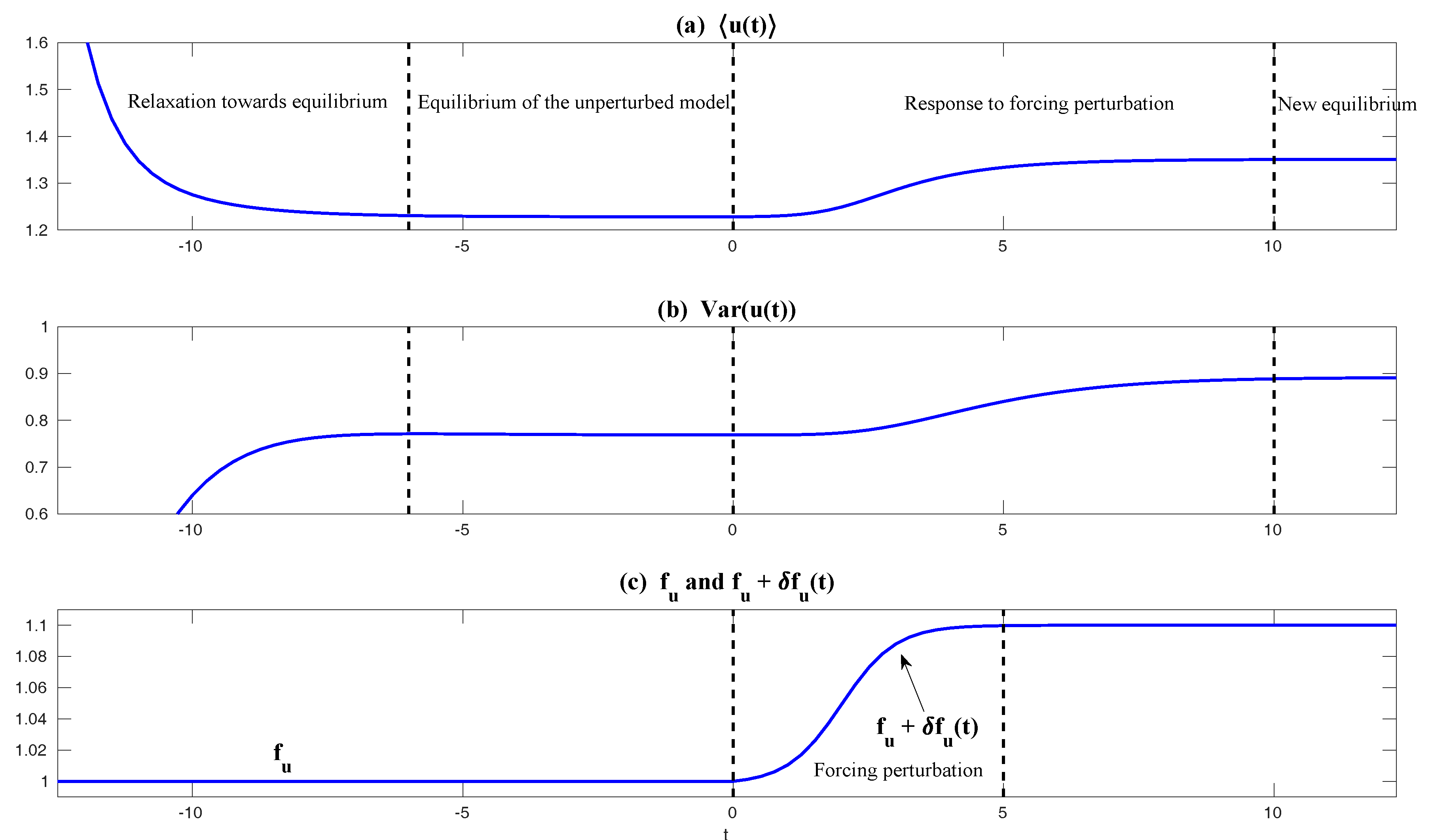
2.3. Intrinsic Information Barrier in Predicting Mean Response to the Change of Forcing
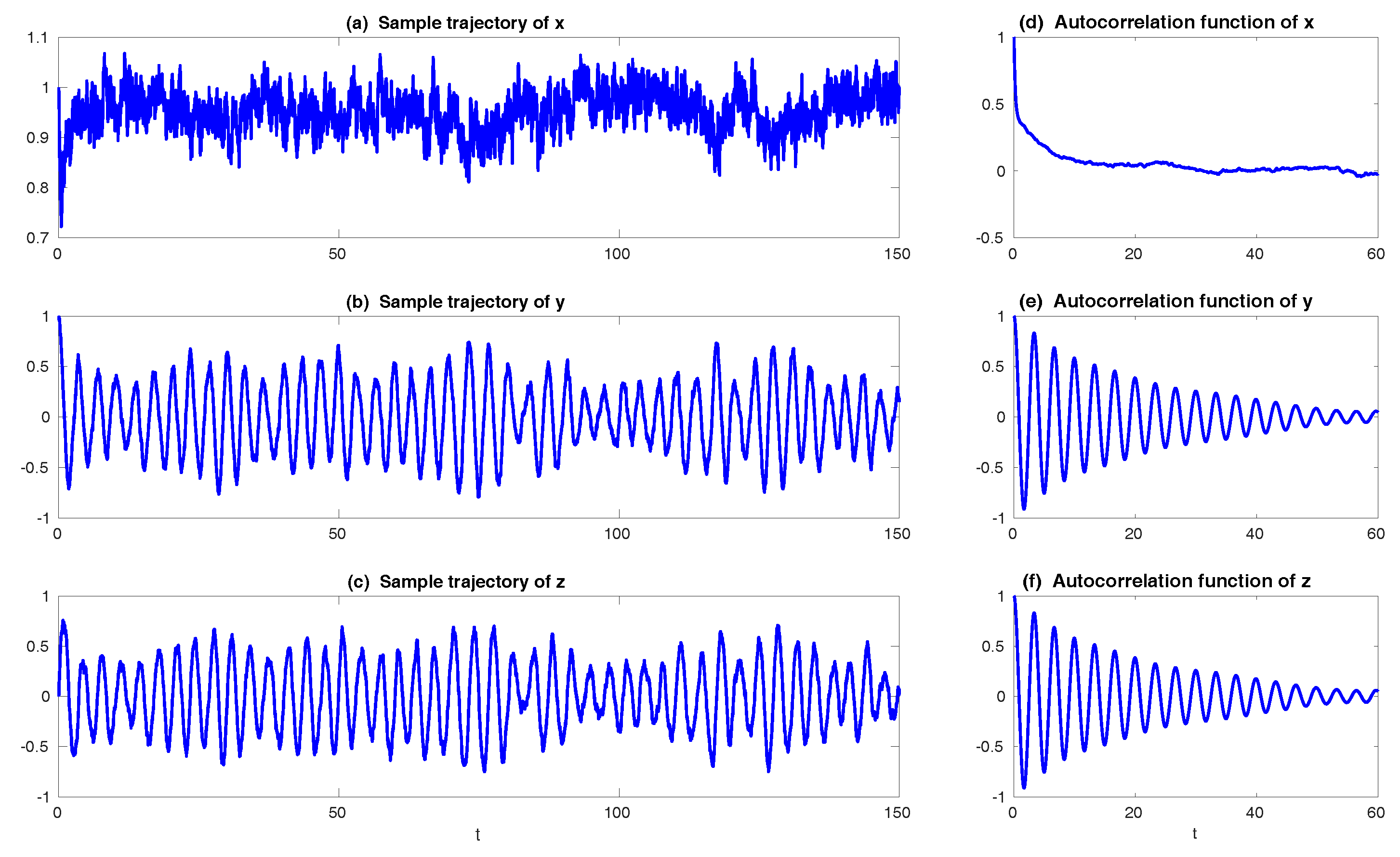
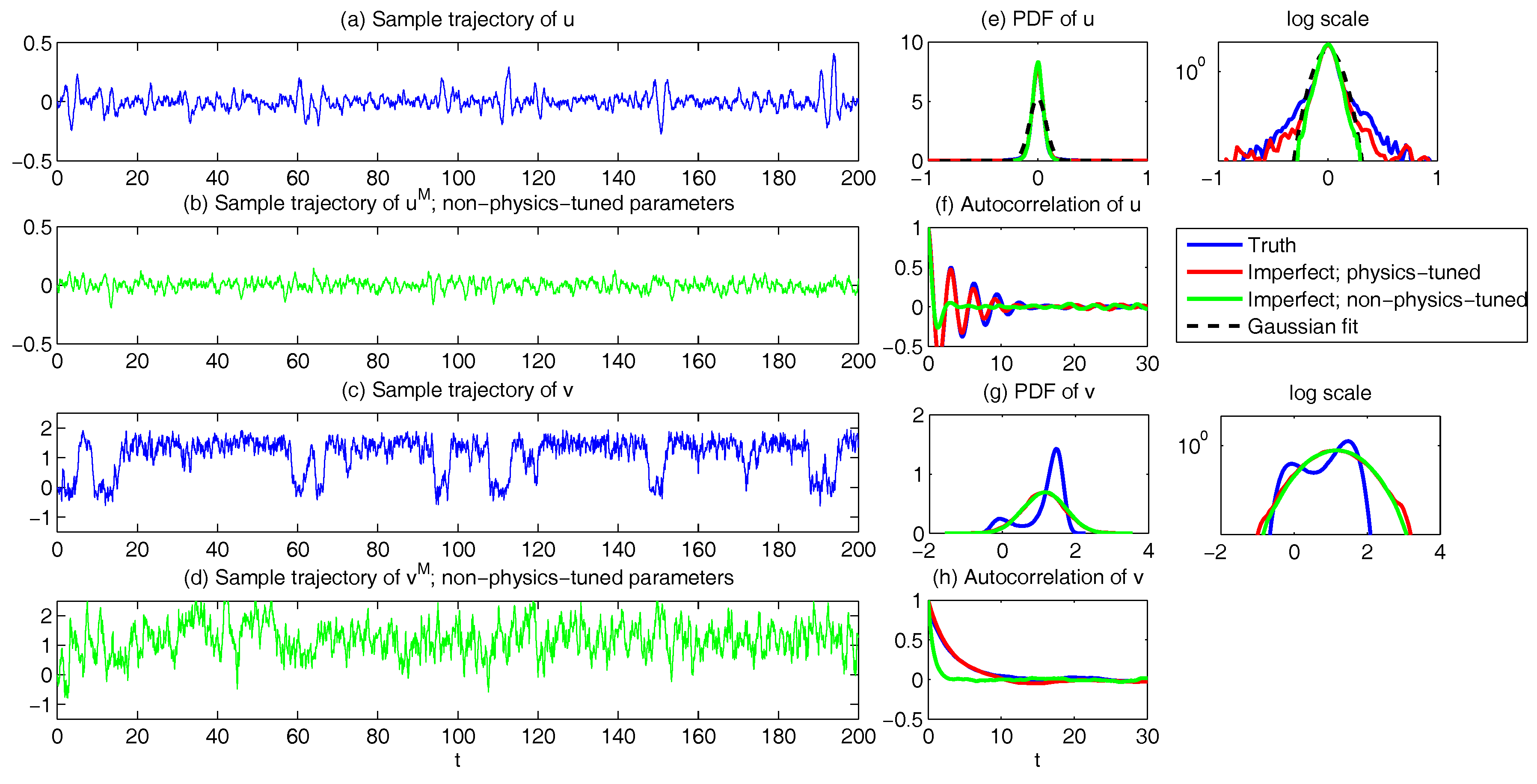
2.4. Slow-Fast System and Reduced Model
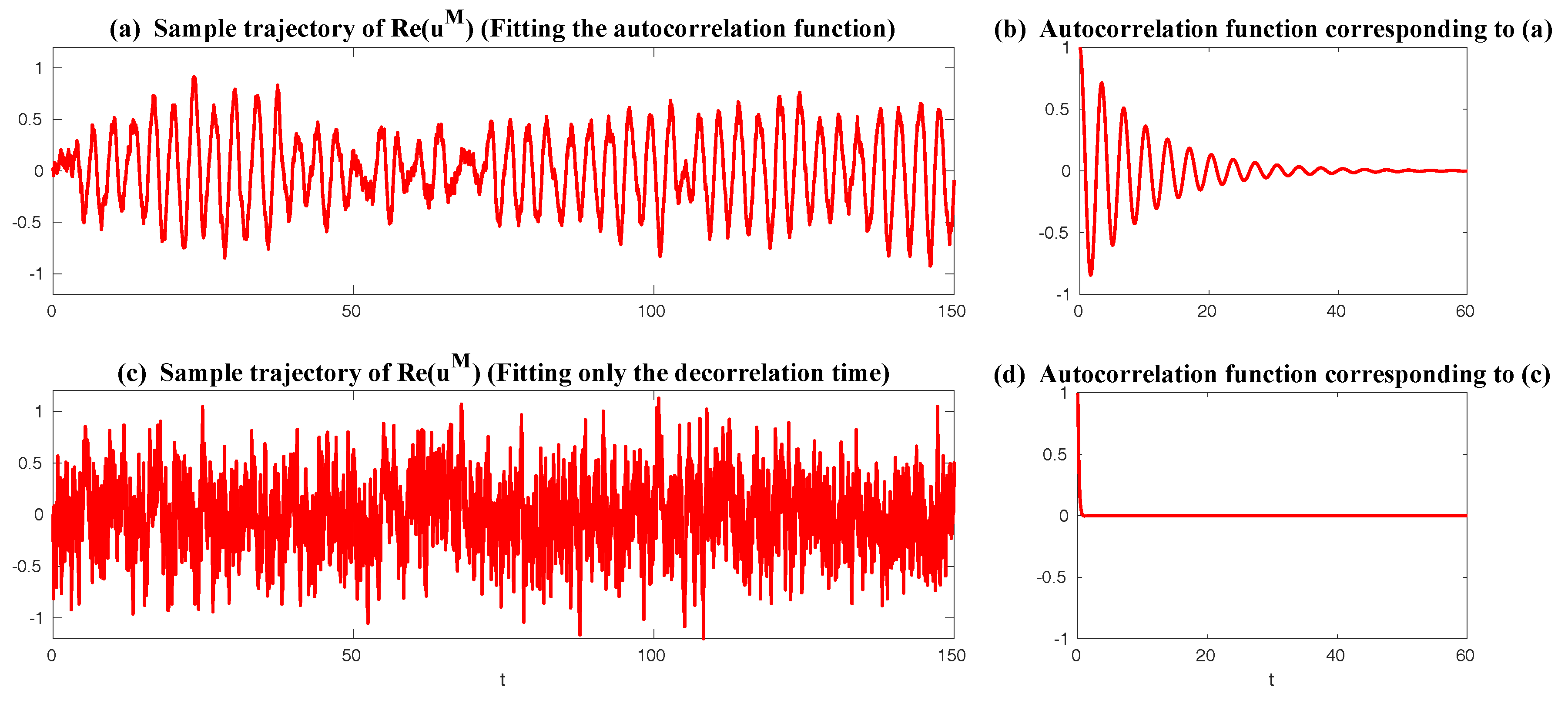
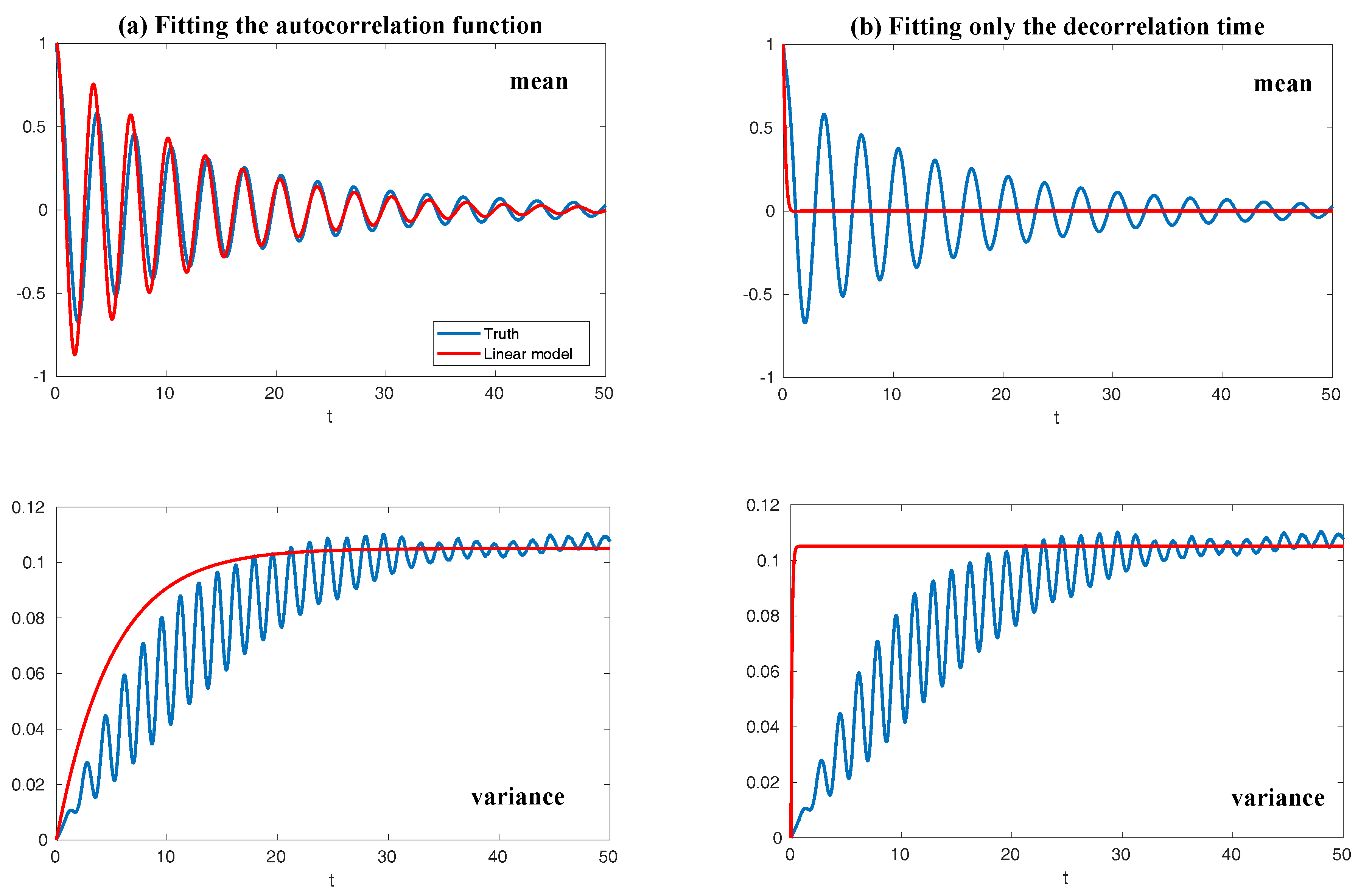
2.5. Fitting Autocorrelation Function of Time Series by a Spectral Information Criteria
3. Quantifying Model Error with Information Theory in State Estimation and Prediction
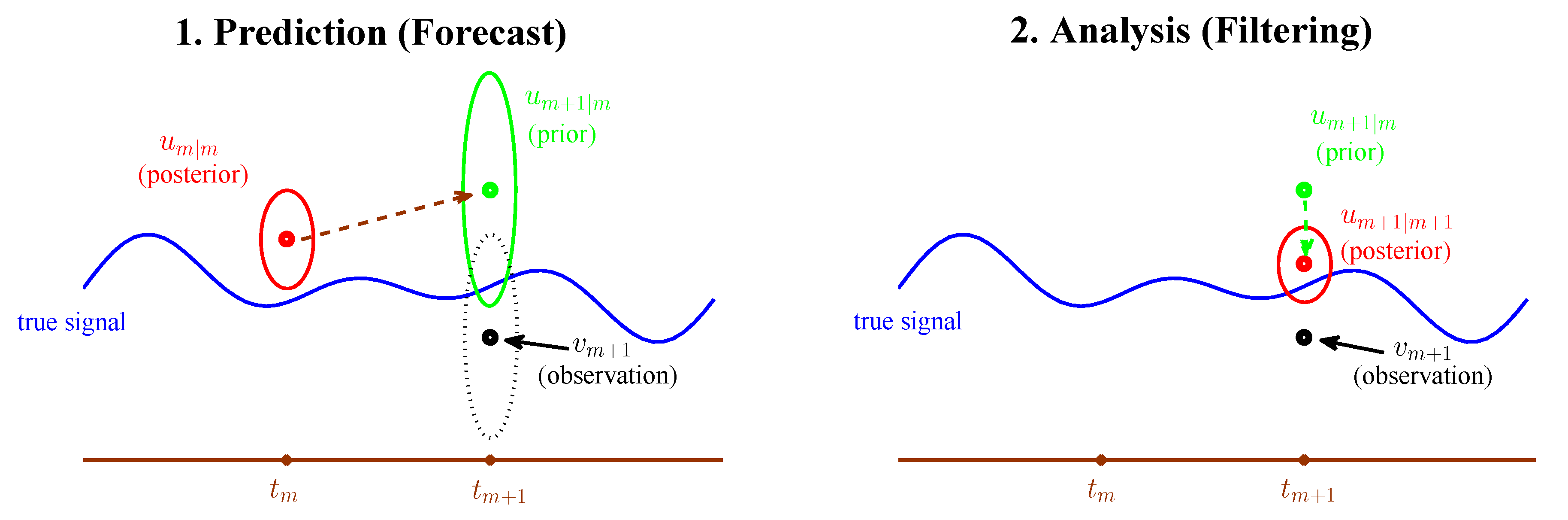
3.1. Kalman Filter, State Estimation and Linear Stochastic Model Prediction
3.2. Asymptotic Behavior of Prediction and Filtering in One-Dimensional Linear Stochastic Models with Model Error
3.2.1. Prediction
3.2.2. Filtering
3.2.3. Comparison
3.3. An Information Theoretical Framework for State Estimation and Prediction
3.3.1. Motivation Examples
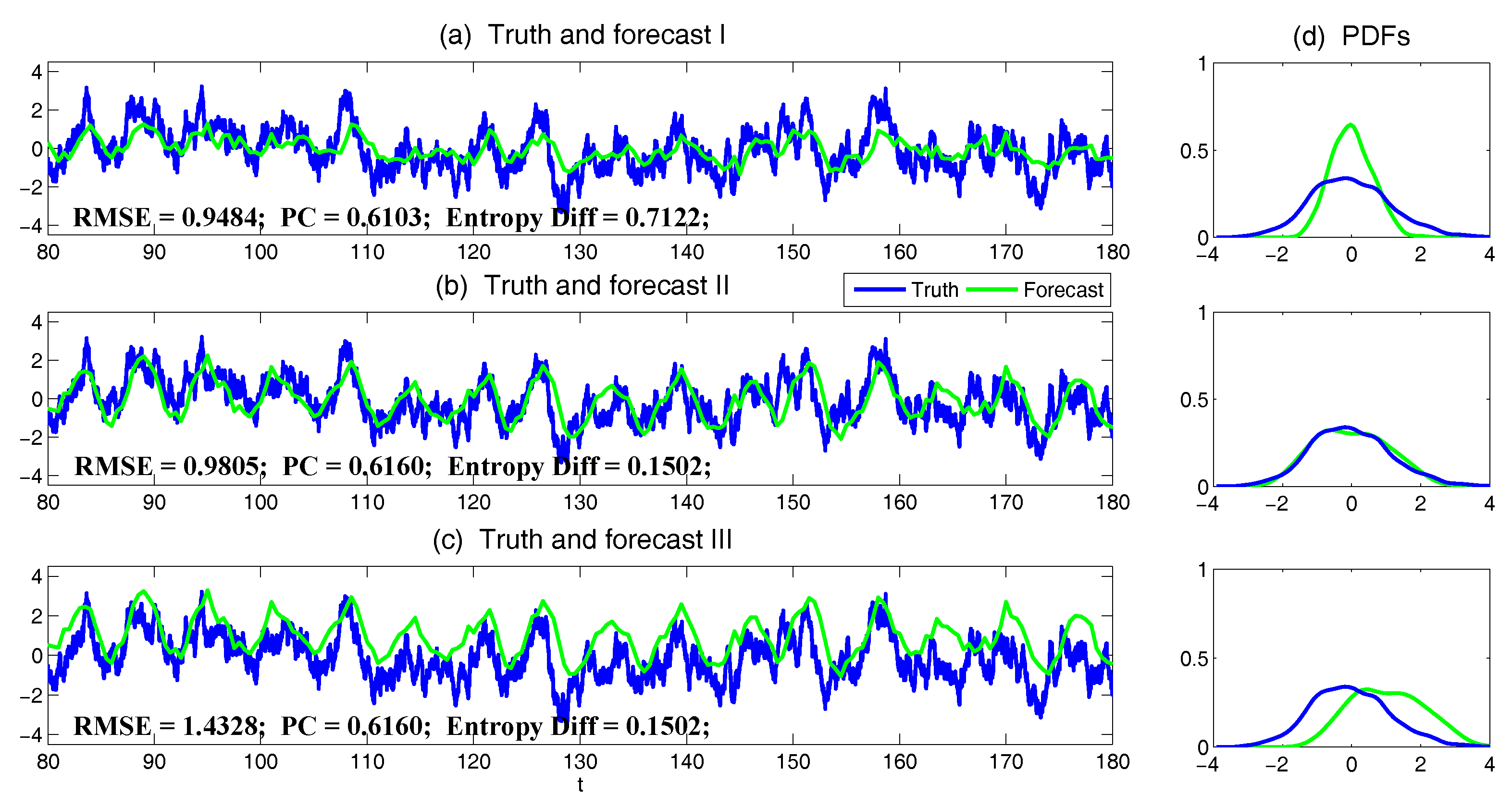
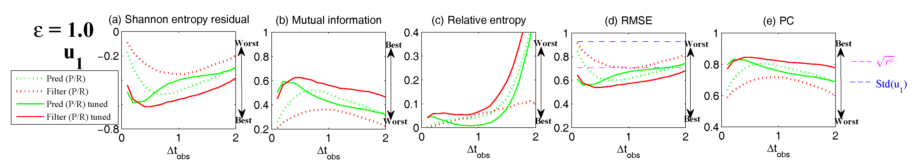
- The root-mean-square error (RMSE):
- The pattern correlation (PC):where and denotes the mean of and , respectively.
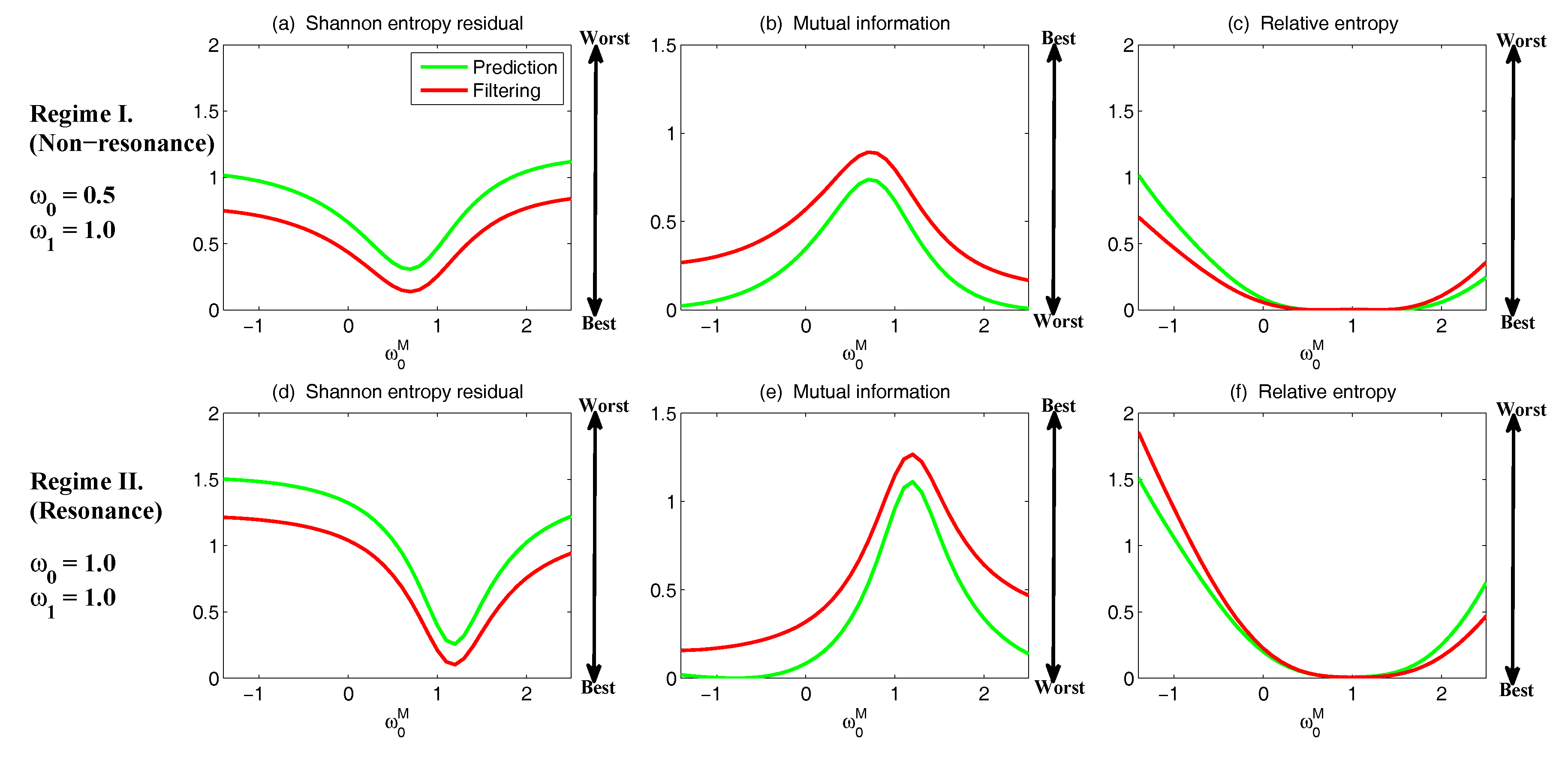
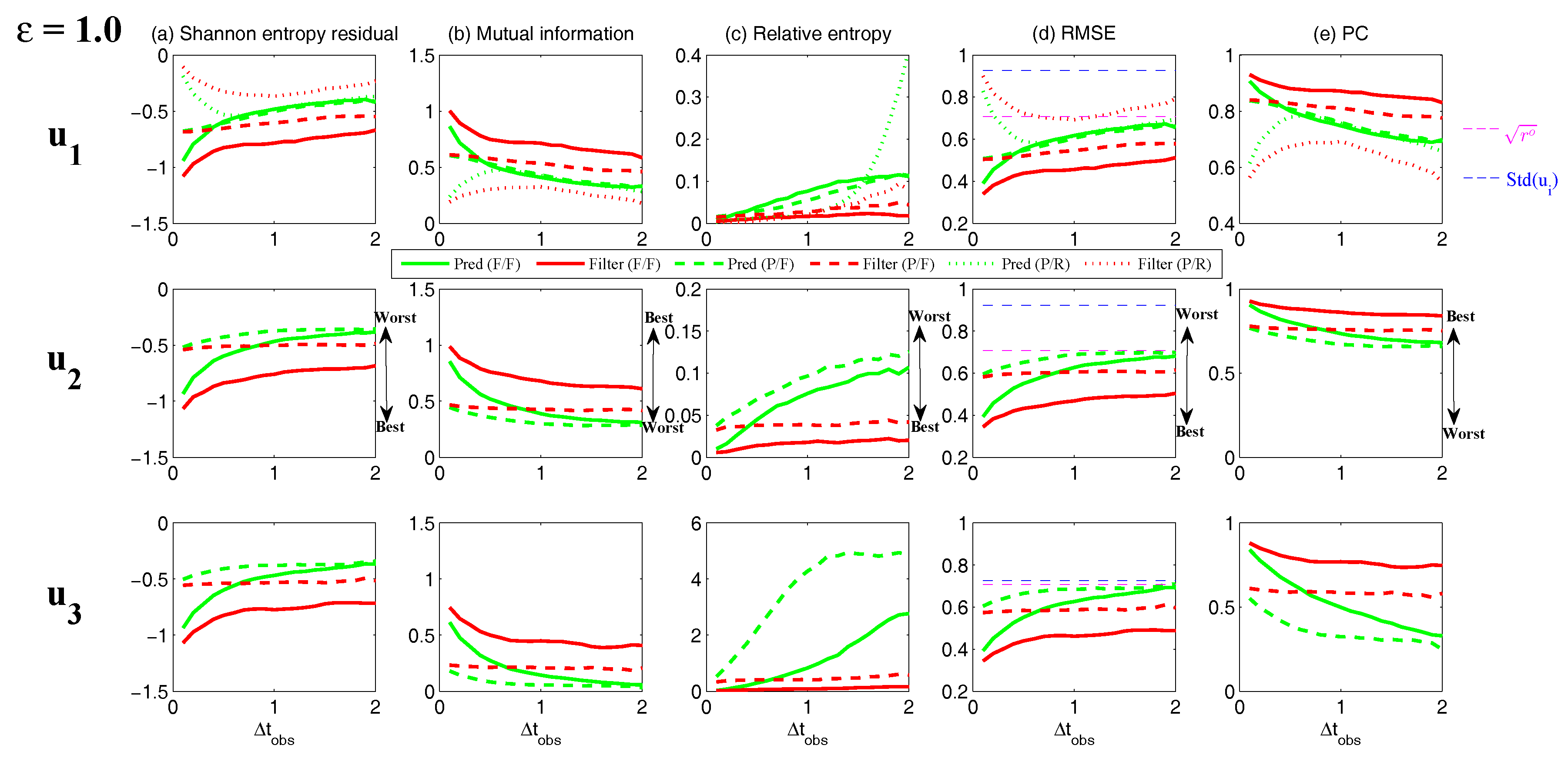
3.3.2. Assessing the Skill of Estimation and Prediction Using Information Theory
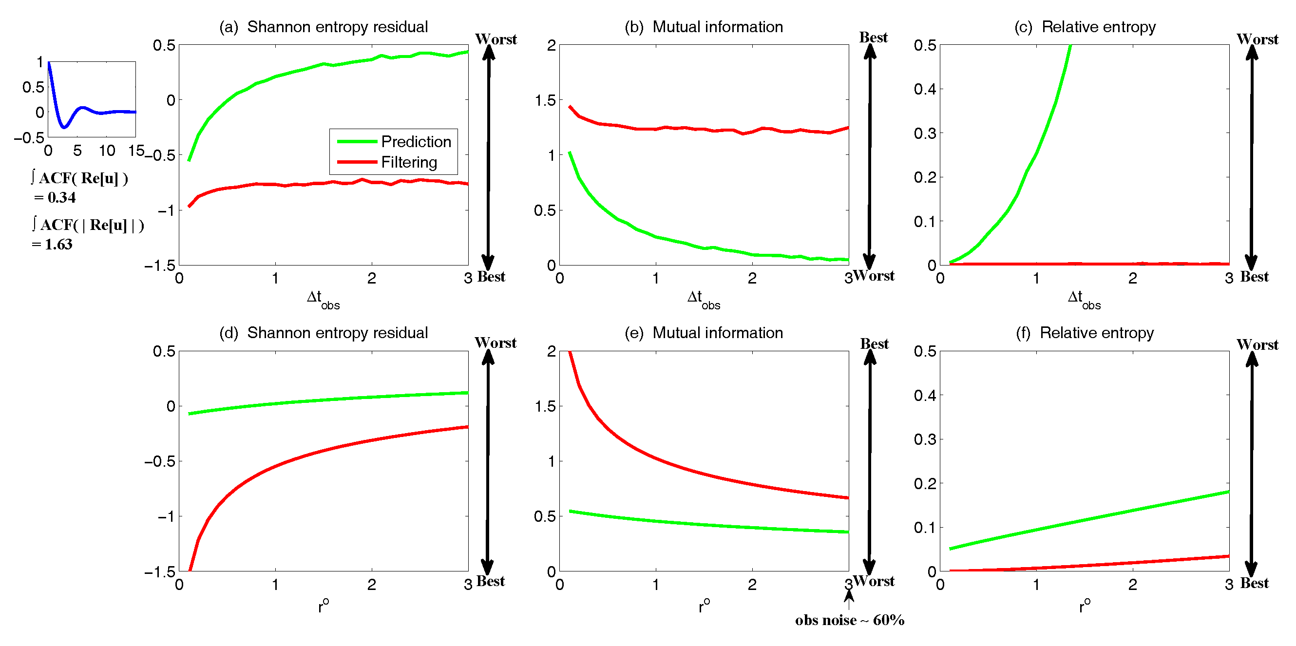
- The Shannon entropy residual,
- The mutual information,
- The relative entropy,
- The Shannon entropy residual (Gaussian framework),
- The mutual information (Gaussian framework),
- The relative entropy (Gaussian framework),
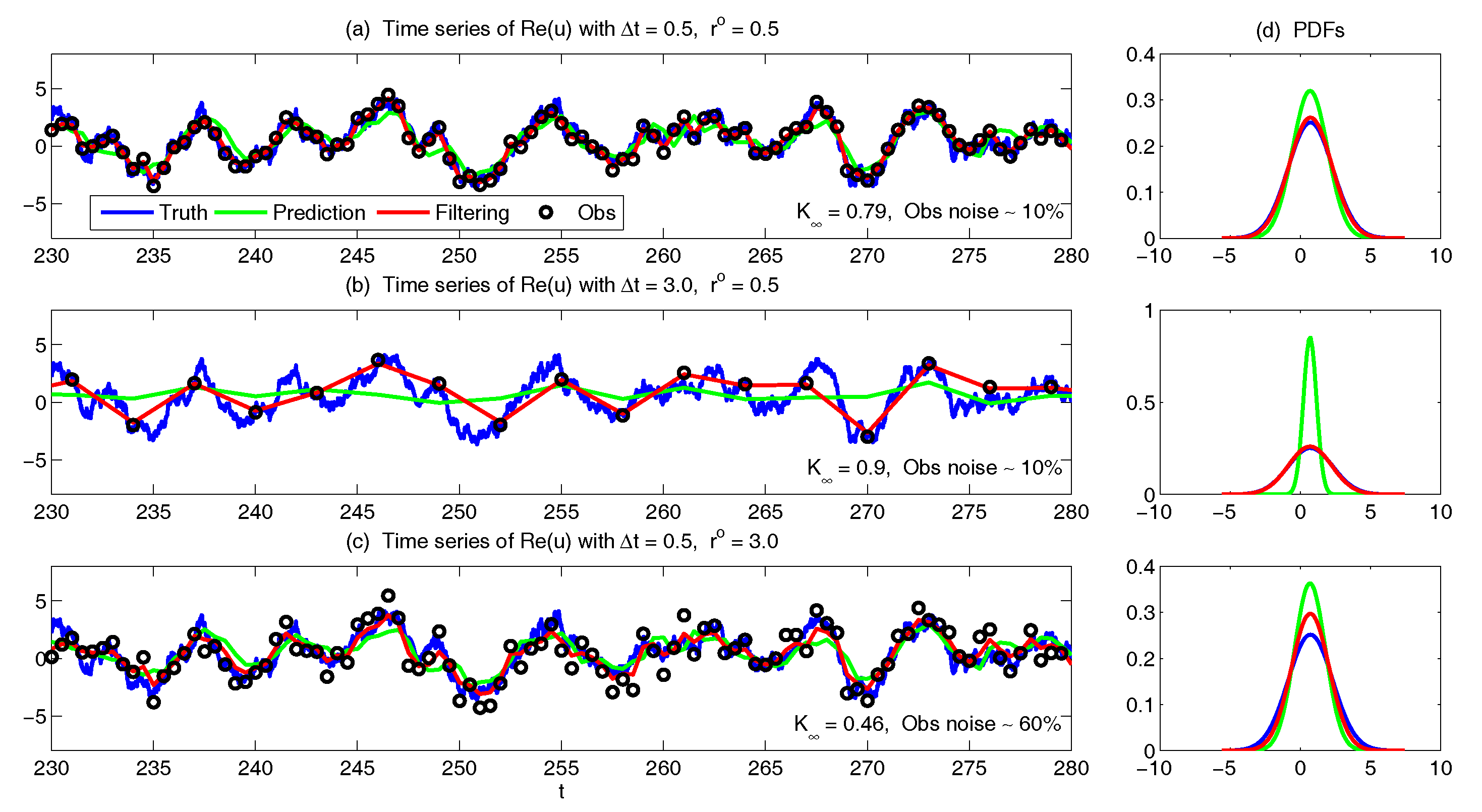
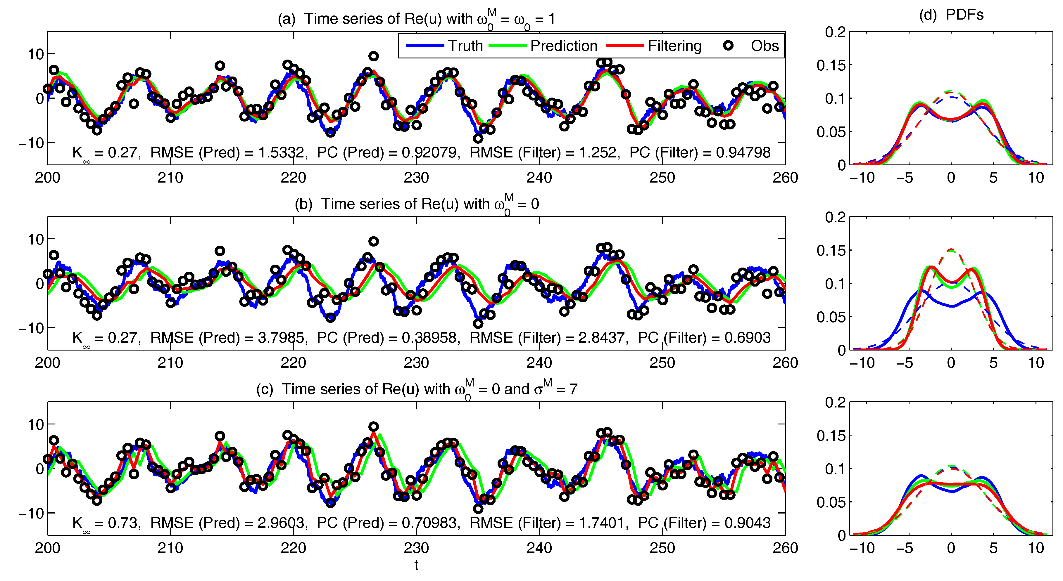
3.4. State Estimation and Prediction for Complex Scalar Forced Ornstein–Uhlenbeck (OU) Processes
3.5. State Estimation and Prediction for Multiscale Slow-Fast Systems
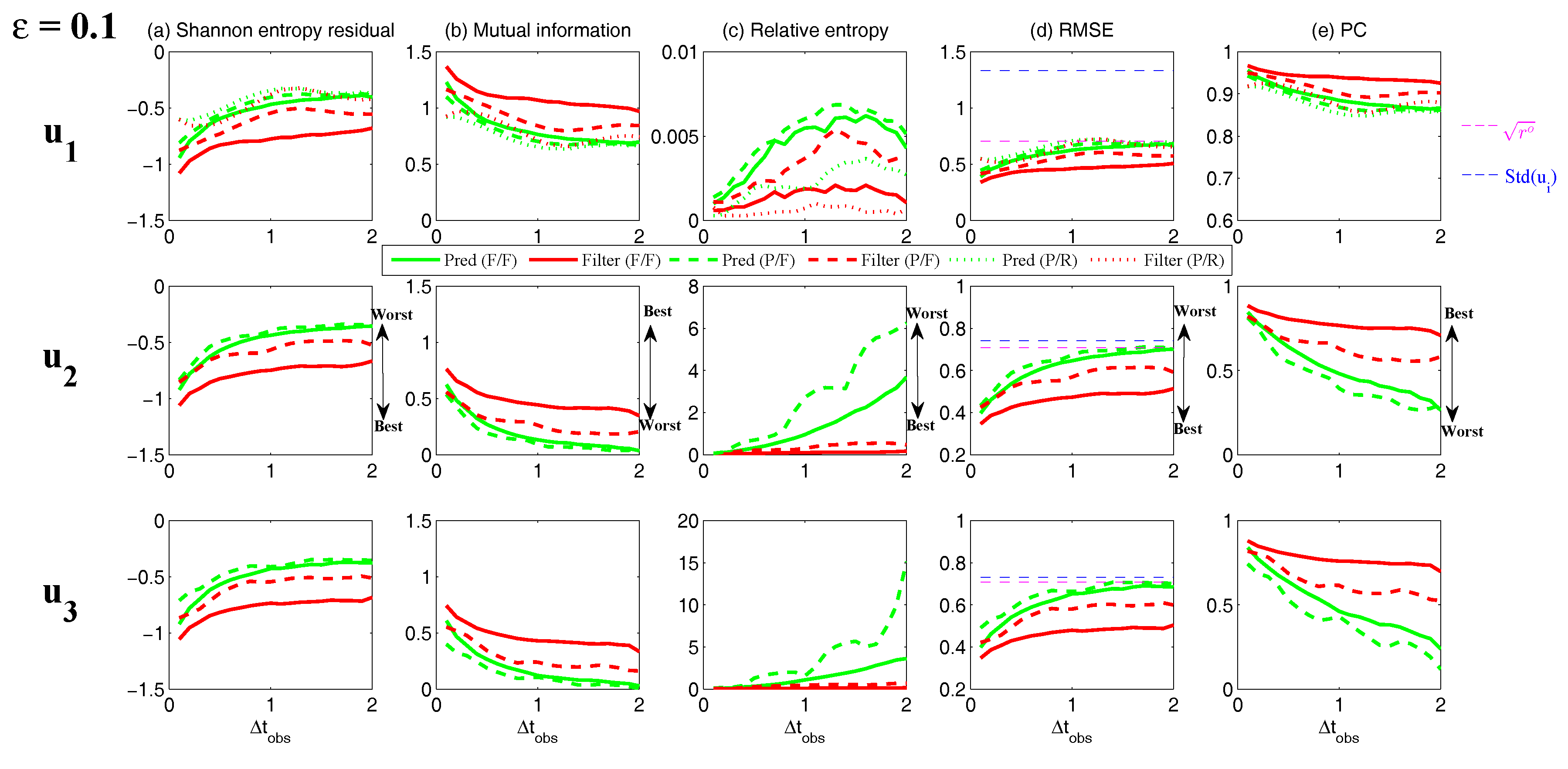
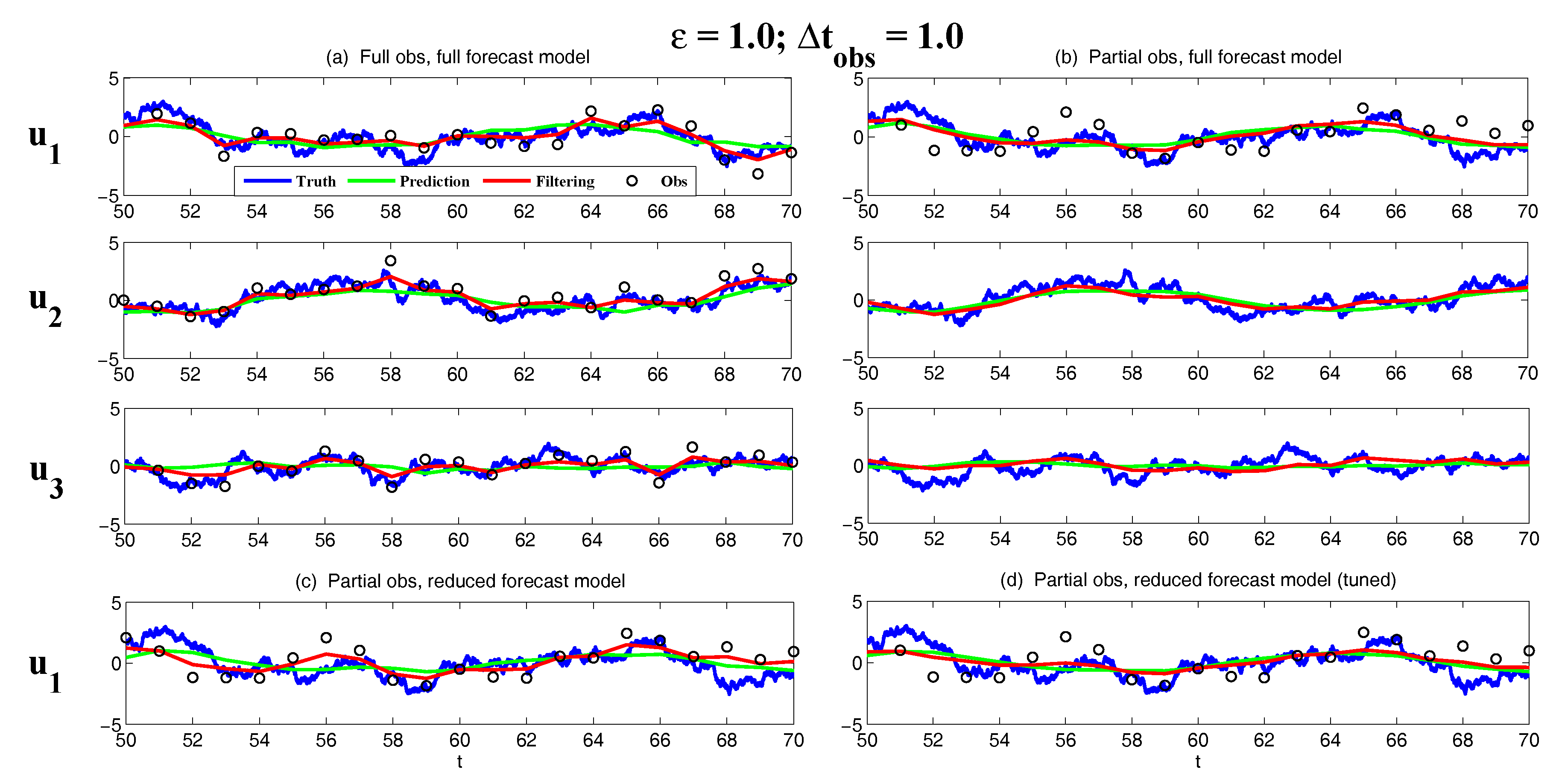
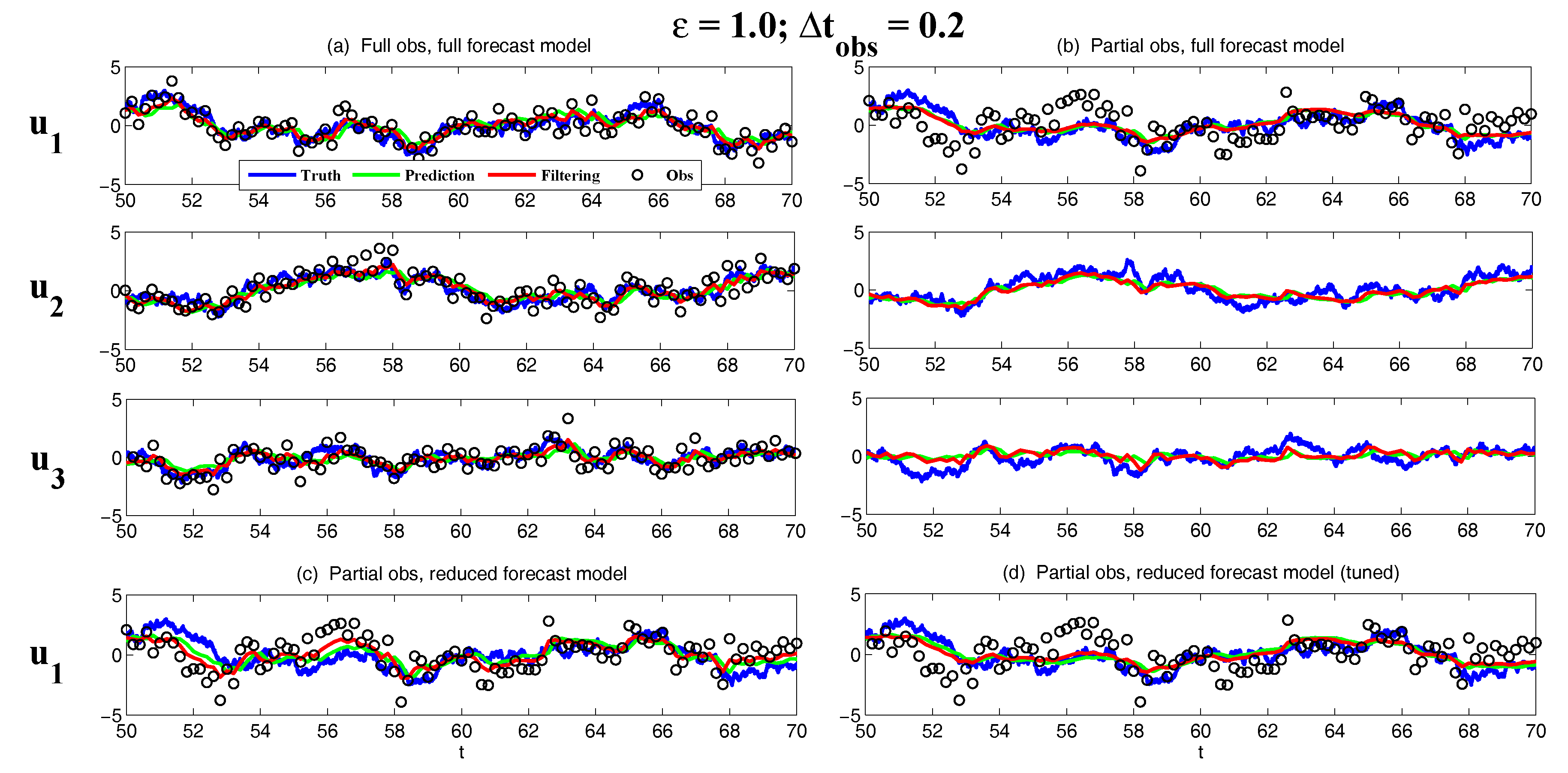
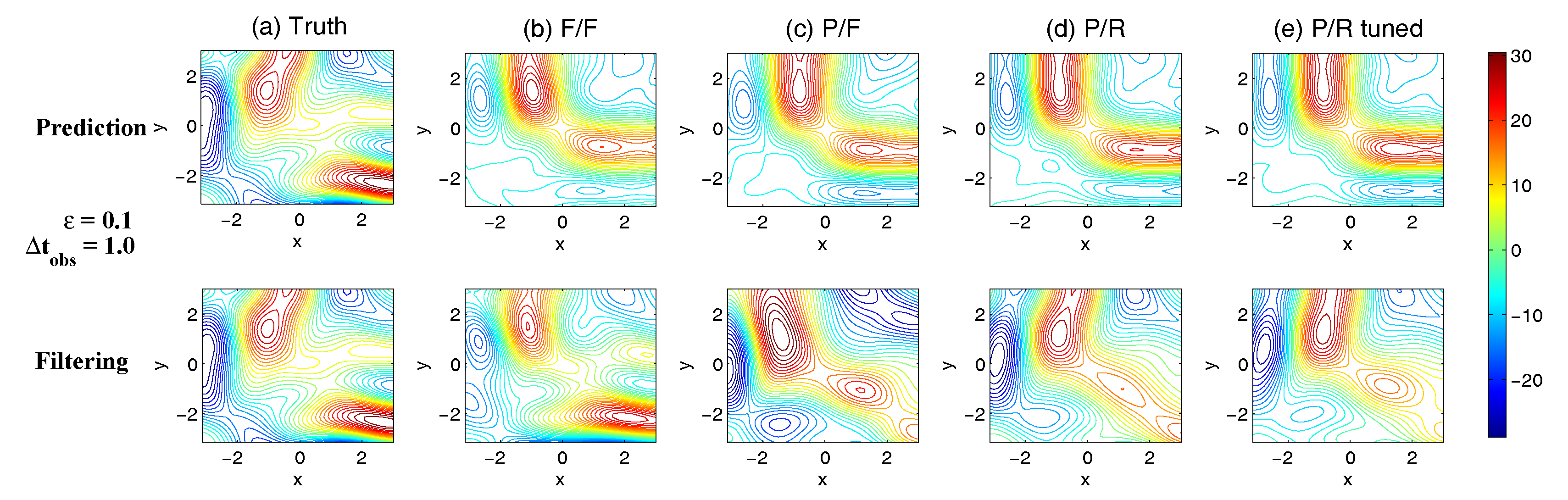
3.5.1. A Linear Coupled Multiscale Slow-Fast System
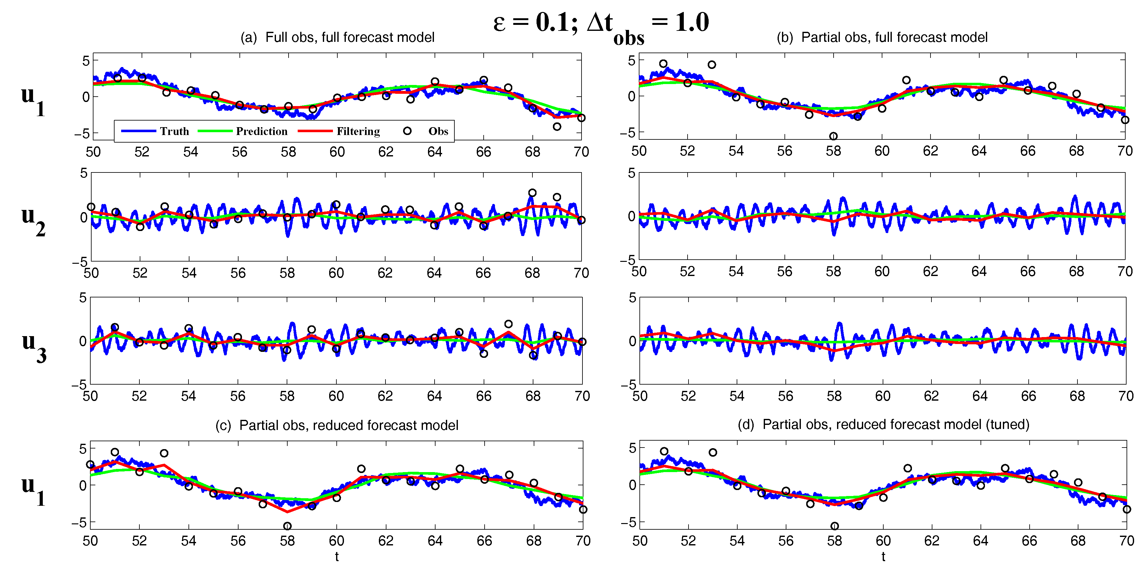
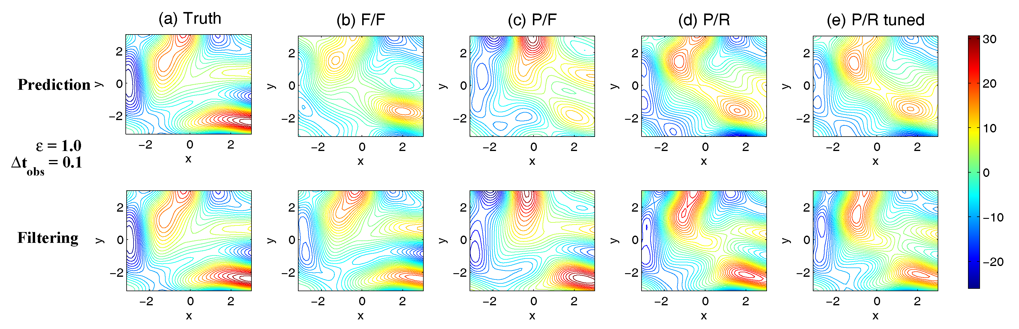
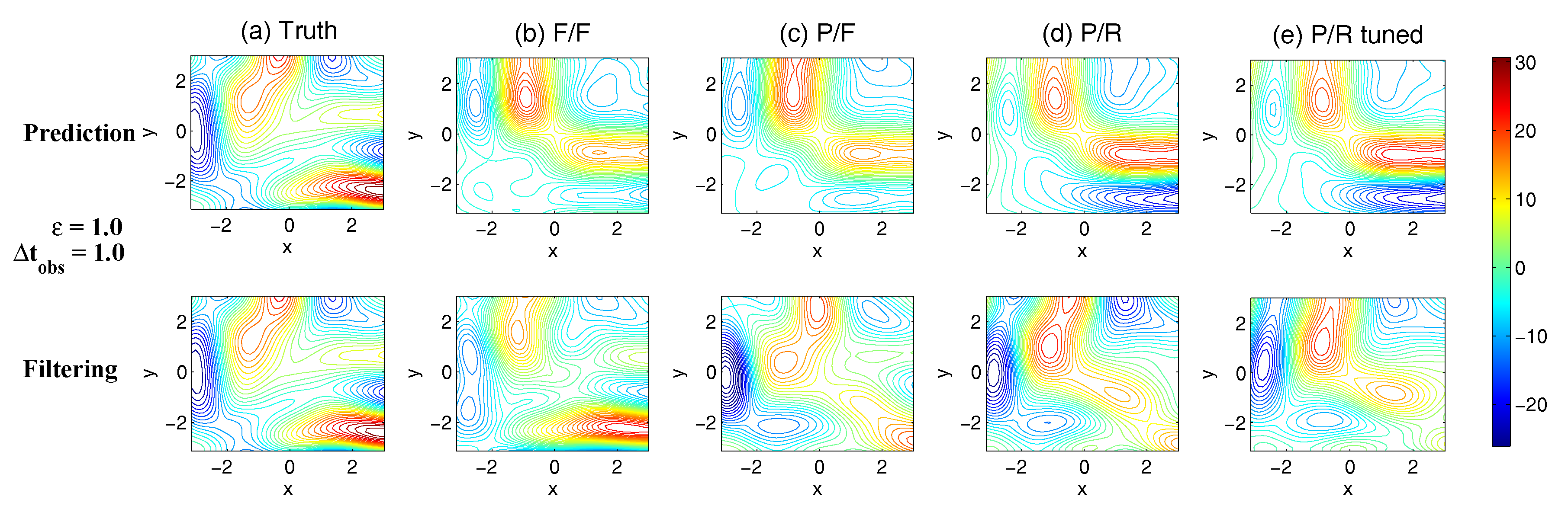
- Full observations, full forecast model (F/F). The observational operator g is an identity such thatThe forecast model is the same as in (105). Although this straightforward setup may not be practical (see below) and can be expensive when a much larger dimension of the system is considered (see next subsection), the results from such a setup can be used as a baseline for testing various modifications and reduced models as will be presented below.
- Partial observations, full forecast model (P/F). The real observations typically involve the superposition of different wave components. It is usually impossible to artificially separate these components from the noisy observations. Therefore, here we let the observational operator be , namely the observation is the combination of the three variables,The forecast model remains the same as that in (105).
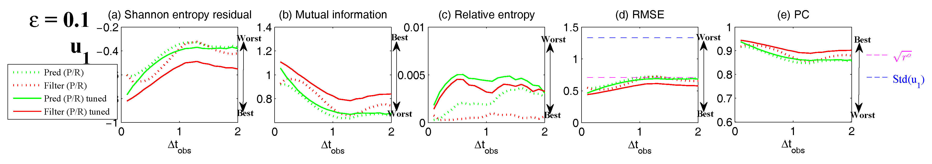
- Partial observations, reduced forecast model (P/R). In practice, only part of the state variables are of particular interest in filtering and prediction. These state variables usually lie in large or resolved scales, such as the GB flow. Therefore, simple reduced forecast models are typically designed to reduce the computational cost and retain the key features in filtering and predicting these variables. To this end, the following reduced forecast model is usedand the observation remains the same as that in (107). Here, we have completely dropped the dependence of on and since their mean is zero according to the setup above.
- Partial observations, reduced forecast model and tuned observational noise level with inflation (P/R tuned). It is easy to notice that in the previous setup (P/R), the signals of and actually become part of the observational noise in filtering and predicting . This is known as the representation error [53,100,150,151,152,153,154]. However, if the original observational noise level is still used in updating the Kalman gain, then the filtering and prediction skill may be affected by the representation error. To resolve this issue, we utilize an inflated in the analysis step to compute the Kalman gain while the other setups remain the same as in the P/R case. Here, the inflated is given bywhere and are the variance of and respectively at the statistical steady state. The inflation in (109) is the most straightforward one. More elaborate inflation techniques can be reached by applying the information theory in the training phase. Nevertheless, with such a simple inflation of the observational noise, the signals of and are treated as part of the observational noise. The estimation of the Kalman gain using the imperfect forecast model (108) is therefore expected to be improved.
3.5.2. Shallow Water Flows
- One geostrophically balanced (GB) mode with eigenvalueThe GB mode is incompressible.
- Two gravity modes with eigenvaluesThe gravity modes are compressible.
4. Information, Sensitivity and Linear Statistical Response—Fluctuation–Dissipation Theorem (FDT)
4.1. Fluctuation–Dissipation Theorem (FDT)
4.1.1. The General Framework
4.1.2. Approximate FDT Methods
4.2. Information Barrier for Linear Reduced Models in Capturing the Response in the Second Order Statistics
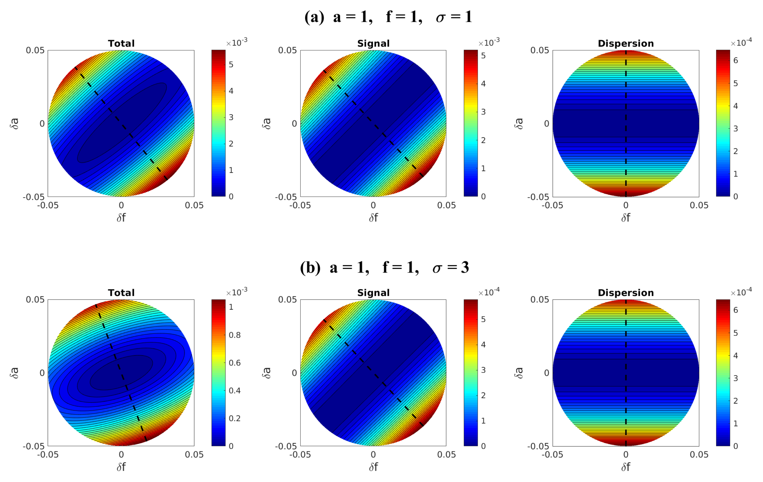
4.3. Information Theory for Finding the Most Sensitive Change Directions
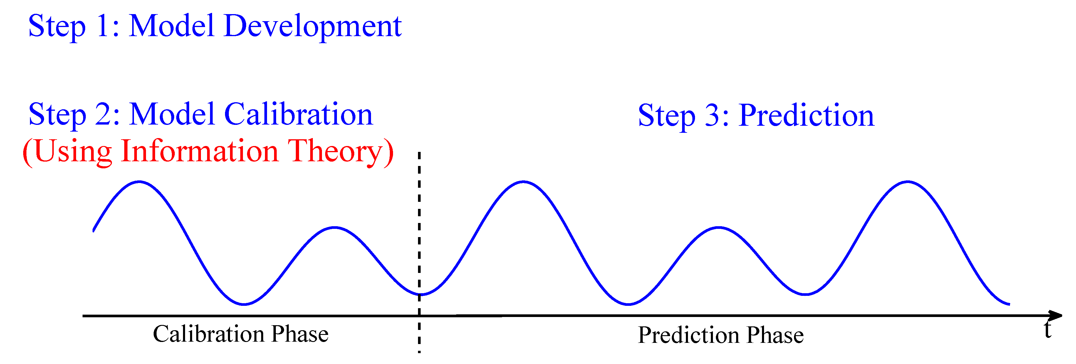
5. Given Time Series, Using Information Theory for Physics-Constrained Nonlinear Stochastic Model for Prediction
5.1. A General Framework
5.2. Model Calibration via Information Theory
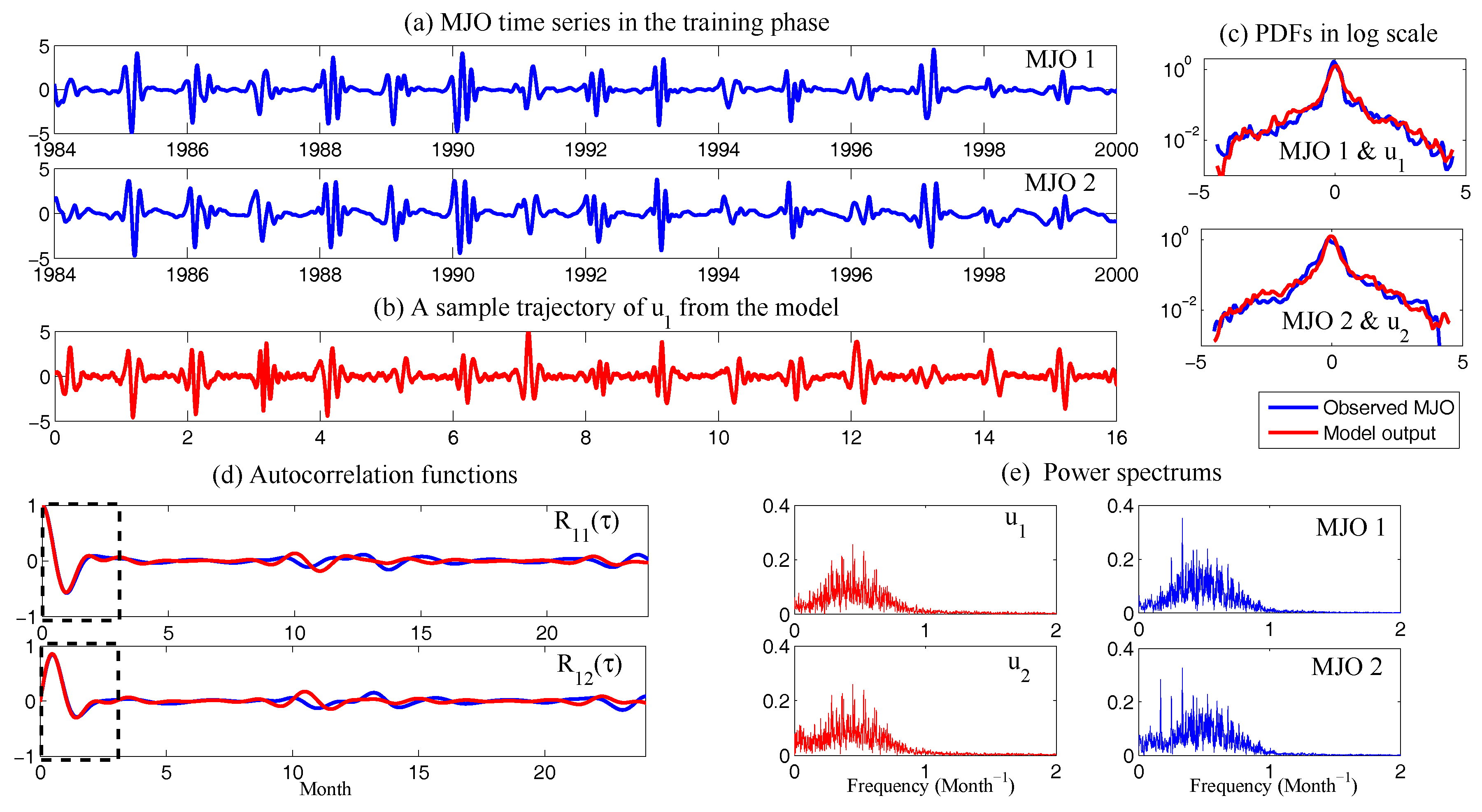
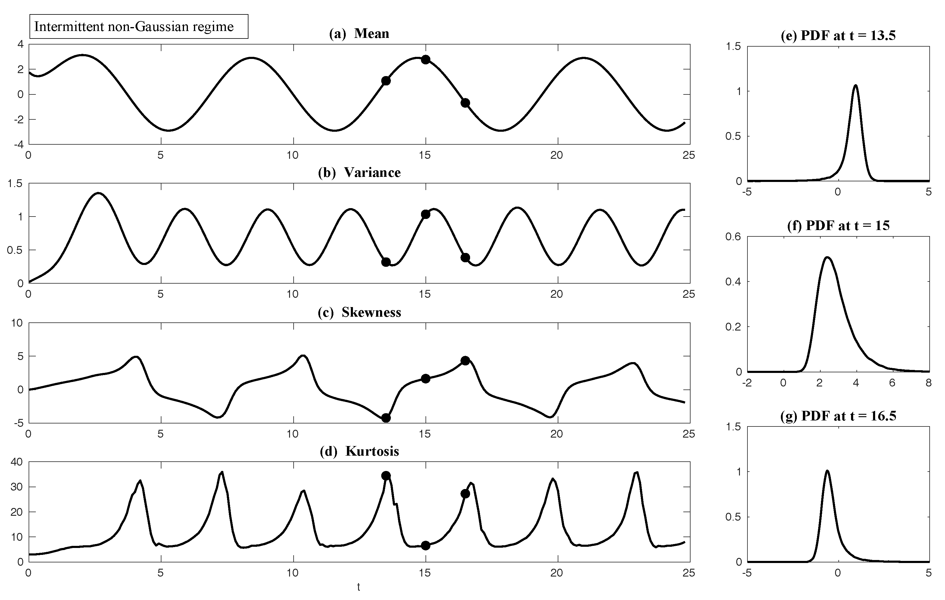
5.3. Applications: Assessing the Predictability Limits of Time Series Associated with Tropical Intraseasonal Variability
6. Reduced-Order Models (ROMs) for Complex Turbulent Dynamical Systems
6.1. Strategies for Reduced-Order Models for Predicting the Statistical Responses and UQ
6.1.1. Turbulent Dynamical System with Energy-Conserving Quadratic Nonlinearity
- is a linear operator representing dissipation and dispersion. Here, L is skew symmetric representing dispersion and D is a negative definite symmetric operator representing dissipative process such as surface drag, radiative damping, viscosity, etc.
- is a bilinear term and it satisfies energy conserving property with .
- The linear dynamical operator expressing energy transfers between the mean field and the stochastic modes (effect due to B), as well as energy dissipation (effect due to D) and non-normal dynamics (effect due to L)
- The positive definite operator expressing energy transfer due to the external stochastic forcing
- The energy flux between different modes due to non-Gaussian statistics (or nonlinear terms) modeled through third-order moments
6.1.2. Modeling the Effect of Nonlinear Fluxes
- Quasilinear Gaussian closure model: The simplest approximation for the closure methods at the first stage should be simply neglecting the nonlinear part entirely [182,183,184]. That is, setThus, the nonlinear energy transfer mechanism will be entirely neglected in this Gaussian closure model. This is the similar idea in the eddy-damped Markovian model where the moment hierarchy is closed at the level of second moments with Gaussian assumption and a much larger eddy-damped parameter is introduced to replace the molecular viscosity [121,185]. Obviously, this crude Gaussian approximation will not work well in general due to the cutoff of the energy flow when strong nonlinear interactions between modes occur. Actually, the deficiency of this crude approximation has been shown under the Lorenz 96 framework, and in a final equilibrium state, there exists only one active mode with a critical wavenumber [11,50]. Such closures are only useful in the weakly nonlinear case where the quasi-linear effects are dominant.
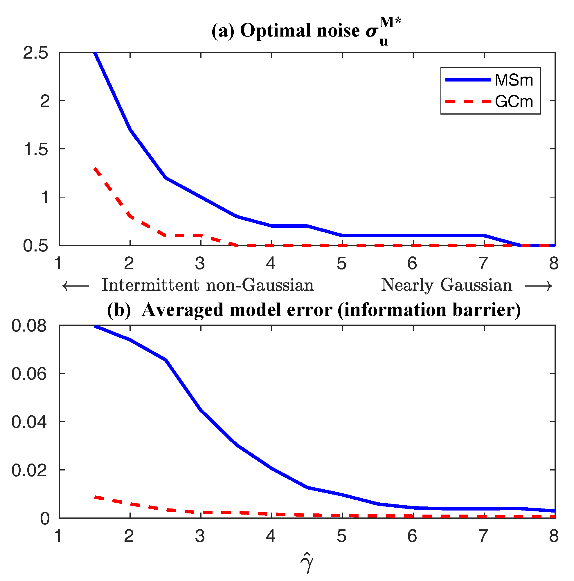
- Models with consistent equilibrium statistics: The next strategy is to construct the simplest closure model with consistent equilibrium statistics. Thus, the direct way is to choose constant damping and noise term scaled with the total variance. We propose two possible choices as in [50] for the damping and noise in (185) below.Gaussian closure 1 (GC1): letGaussian closure 2 (GC2): letAbove, only two scalar model parameters are introduced, and represents the identity matrix. GC1 is the familiar strategy of adding constant damping and white noise forcing to represent nonlinear interaction; GC2 scales with the total variance (or total statistical energy) so that the model sensitivity can be further improved as the system is perturbed. From both GC1 and GC2, we introduce uniform additional damping rate for each spectral mode controlled by a single scalar parameter , while the additional noise with variance is added to make sure climate fidelity in equilibrium.The statistical model closure is used to approximate the third-order moments in the true dynamics, thus the exponents of the total energy in GC2 should be consistent in scaling dimension. In the positive-definite part , it calibrates the rate of energy injected into the spectral mode due to nonlinear effect in the order . The factor scales with the total energy with exponent so that the corrections keep consistent with the third-order moment approximations; In the negative damping rate , the scaling function is used to characterize the amount of energy that flows out the spectral mode due to nonlinear interactions. Scaling factor with a square-root of the total energy with exponent is applied for this damping rate multiplying the variance in order to make it consistent in scaling dimension with third moments.However, the damping and noise are chosen empirically without consideration about the true dynamical features in each mode. A more sophisticated strategy with slightly more complexity in computation is to introduce the damping and noise judiciously according to the linearized dynamics. Then, climate consistency for each mode can be satisfied automatically.
- Modified quasi-Gaussian (MQG) closure with equilibrium statistics: In this modified quasi-Gaussian closure model originally proposed in [11,45], we exploit more about the true nonlinear energy transfer mechanism from the equilibrium statistical information. Thus, the additional damping and noise proposed as before are calibrated through the equilibrium nonlinear flux by lettingis the effective damping from equilibrium, and is the effective noise from the positive-definite component. Unperturbed equilibrium statistics in the nonlinear flux are used to calibrate the higher-order moments as additional energy sink and source. The true equilibrium higher-order flux can be calculated without error from first and second order moments in from the unperturbed true dynamics (180) in steady state following the steady state statistical solution relation:where are the negative and positive definite components in the unperturbed equilibrium nonlinear flux . Since exact model statistics are used in the imperfect model approximations, the true mechanism in the nonlinear energy transfer can be modeled under this first correction form. This is the similar idea used for measuring higher order interactions in [45], where more sophisticated and expensive calibrations are required to make that model work there.
6.1.3. A Reduced-Order Statistical Energy Model with Optimal Consistency and Sensitivity
- (i).
- Higher-order corrections from equilibrium statistics: In the first part of the correction using the damping and noise operator as , unperturbed equilibrium statistics in the nonlinear flux are used to calibrate the higher-order moments as additional energy sink and source following the procedure in (189). Therefore, the equilibrium statistics can be guaranteed to be consistent with the truth, and the true energy mechanism can be restored.
- (ii).
- Additional damping and noise to model changes in nonlinear flux: The above corrections in step (i) by using equilibrium information for nonlinear flux is found to be insufficient for accurate prediction in the reduced-order methods since the scheme is only marginally stable and the energy transferring mechanism may change with large deviation from the equilibrium case when external perturbations are applied. Thus, we also introduce the additional damping and noise as from (187). is just a constant scalar parameter to add uniform dissipation on each mode, and is the further correction as an additional energy source to maintain climate fidelity.
- (iii).
- Statistical energy scaling to improve model sensitivity: Still note that these additional parameters are added regardless of the true nonlinear perturbed energy mechanism where only unperturbed equilibrium statistics are used. To capture the responses to a specific perturbation forcing, it is better to make the imperfect model parameters change adaptively according to the total energy structure. Considering this, the additional damping and noise corrections are scaled with factors related with the total statistical variance as>
6.1.4. Calibration Strategy
6.2. Physics-Tuned Linear Regression Models for Hidden (Latent) Variables
6.3. Predicting Passive Tracer Extreme Events
- Whether a linear Gaussian dynamics in approximating the advection flow is able to capture tracer non-Gaussian statistical structures?
- How to design an unambiguous reduced-order stochastic modeling strategy with high prediction skill of the tracer field?
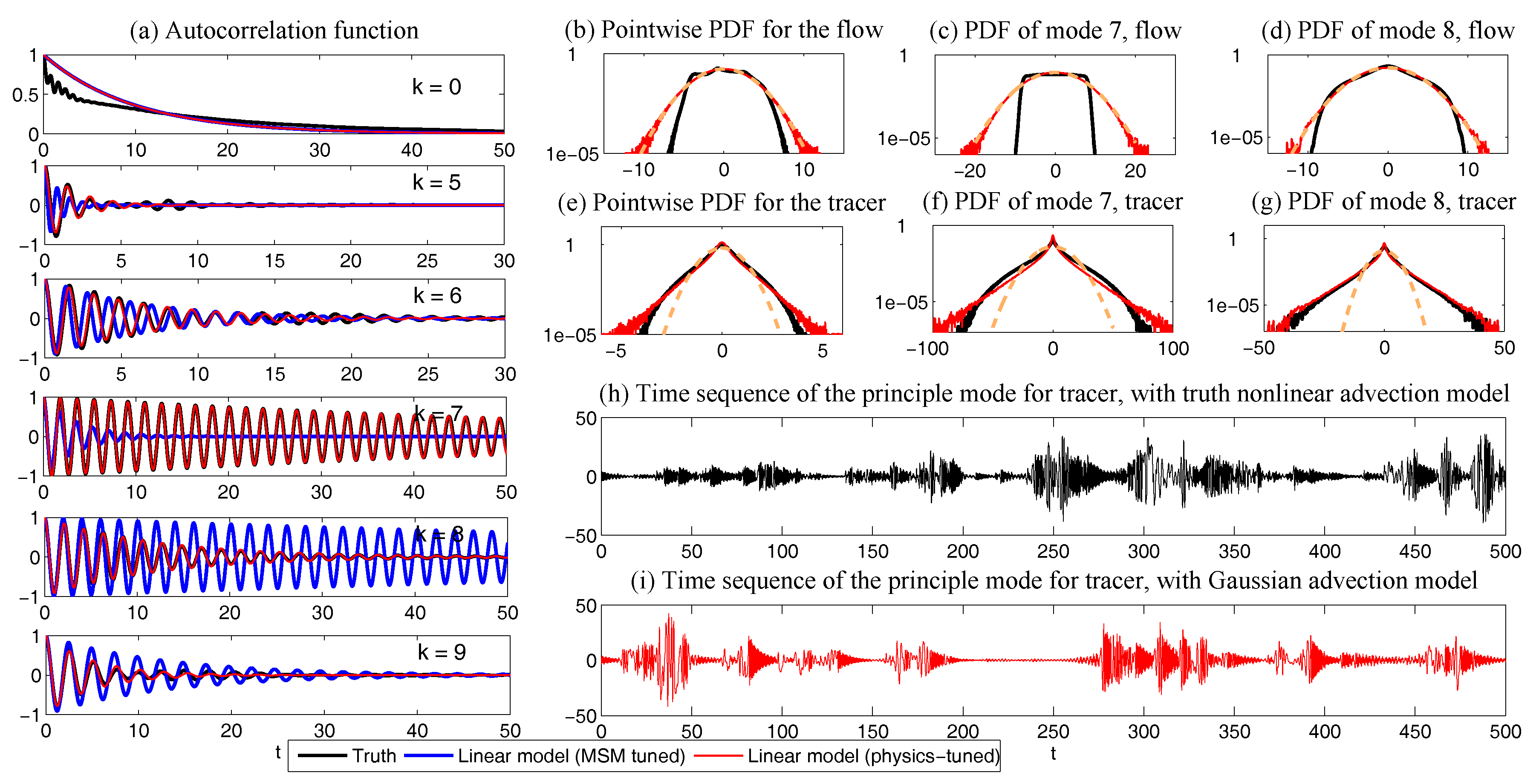
6.3.1. Approximating Nonlinear Advection Flow Using Physics-Tuned Linear Regression Model
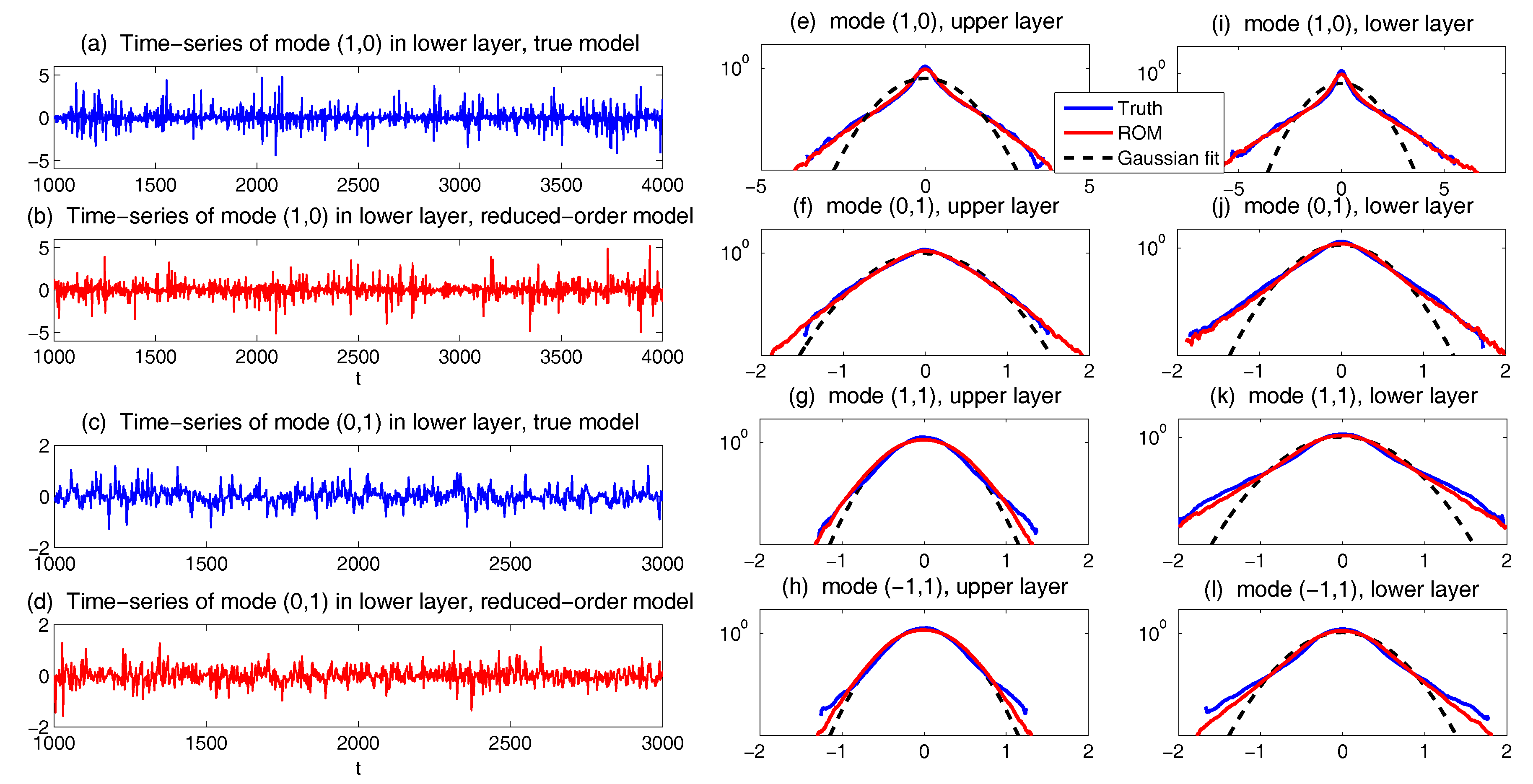
6.3.2. Predicting Passive Tracer Extreme Events with Low-Order Stochastic Models
- Properly reflecting the nonlinear energy mechanism from the true system.
- Imperfect stochastic model consistency in equilibrium statistics and autocorrelation functions.
7. Conclusions
Author Contributions
Funding
Acknowledgments
Conflicts of Interest
Appendix A. Derivations of Fisher Information from Relative Entropy
Appendix B. Details of the Canonical Model for Low Frequency Atmospheric Variability
Appendix C. Augmented System for Prediction and Filtering Distributions
Appendix C.1. Augmented System for Prediction
Appendix C.2. Augmented System for Filtering
Appendix D. Possible Non-Gaussian PDFs of a Linear Model with Time-Periodic Forcing Based on the Sample Points in a Single Trajectory

References
- Majda, A.J. Introduction to Turbulent Dynamical Systems in Complex Systems; Springer: Berlin, Germany, 2016. [Google Scholar]
- Majda, A.; Wang, X. Nonlinear Dynamics and Statistical Theories for Basic Geophysical Flows; Cambridge University Press: Cambridge, UK, 2006. [Google Scholar]
- Strogatz, S.H. Nonlinear Dynamics and Chaos: With Applications to Physics, Biology, Chemistry, and Engineering; CRC Press: Boca Raton, FL, USA, 2018. [Google Scholar]
- Baleanu, D.; Machado, J.A.T.; Luo, A.C. Fractional Dynamics and Control; Springer Science & Business Media: Berlin, Germany, 2011. [Google Scholar]
- Deisboeck, T.; Kresh, J.Y. Complex Systems Science in Biomedicine; Springer Science & Business Media: Berlin, Germany, 2007. [Google Scholar]
- Stelling, J.; Kremling, A.; Ginkel, M.; Bettenbrock, K.; Gilles, E. Foundations of Systems Biology; MIT Press: Cambridge, MA, USA, 2001. [Google Scholar]
- Sheard, S.A.; Mostashari, A. Principles of complex systems for systems engineering. Syst. Eng. 2009, 12, 295–311. [Google Scholar] [CrossRef]
- Majda, A. Introduction to PDEs and Waves for the Atmosphere and Ocean; American Mathematical Society: Providence, RI, USA, 2003; Volume 9. [Google Scholar]
- Wiggins, S. Introduction to Applied Nonlinear Dynamical Systems and Chaos; Springer Science & Business Media: Berlin, Germany, 2003; Volume 2. [Google Scholar]
- Majda, A.J.; Branicki, M. Lessons in uncertainty quantification for turbulent dynamical systems. Discret. Contin. Dyn. Syst. A 2012, 32, 3133–3221. [Google Scholar] [Green Version]
- Sapsis, T.P.; Majda, A.J. A statistically accurate modified quasilinear Gaussian closure for uncertainty quantification in turbulent dynamical systems. Phys. D Nonlinear Phenom. 2013, 252, 34–45. [Google Scholar] [CrossRef]
- Mignolet, M.P.; Soize, C. Stochastic reduced order models for uncertain geometrically nonlinear dynamical systems. Comput. Methods Appl. Mech. Eng. 2008, 197, 3951–3963. [Google Scholar] [CrossRef]
- Kalnay, E. Atmospheric Modeling, Data Assimilation and Predictability; Cambridge University Press: Cambridge, UK, 2003. [Google Scholar]
- Lahoz, W.; Khattatov, B.; Ménard, R. Data assimilation and information. In Data Assimilation; Springer: Berlin, Germany, 2010; pp. 3–12. [Google Scholar]
- Majda, A.J.; Harlim, J. Filtering Complex Turbulent Systems; Cambridge University Press: Cambridge, UK, 2012. [Google Scholar]
- Evensen, G. Data Assimilation: The Ensemble Kalman Filter; Springer Science & Business Media: Berlin, Germany, 2009. [Google Scholar]
- Law, K.; Stuart, A.; Zygalakis, K. Data Assimilation: A Mathematical Introduction; Springer: Berlin, Germany, 2015; Volume 62. [Google Scholar]
- Palmer, T.N. A nonlinear dynamical perspective on model error: A proposal for non-local stochastic-dynamic parametrization in weather and climate prediction models. Q. J. R. Meteorol. Soc. 2001, 127, 279–304. [Google Scholar] [CrossRef]
- Orrell, D.; Smith, L.; Barkmeijer, J.; Palmer, T. Model error in weather forecasting. Nonlinear Process. Geophys. 2001, 8, 357–371. [Google Scholar] [CrossRef] [Green Version]
- Hu, X.M.; Zhang, F.; Nielsen-Gammon, J.W. Ensemble-based simultaneous state and parameter estimation for treatment of mesoscale model error: A real-data study. Geophys. Res. Lett. 2010, 37. [Google Scholar] [CrossRef] [Green Version]
- Benner, P.; Gugercin, S.; Willcox, K. A survey of projection-based model reduction methods for parametric dynamical systems. SIAM Rev. 2015, 57, 483–531. [Google Scholar] [CrossRef]
- Majda, A.J. Challenges in climate science and contemporary applied mathematics. Commun. Pure Appl. Math. 2012, 65, 920–948. [Google Scholar] [CrossRef]
- Giannakis, D.; Majda, A.J. Quantifying the predictive skill in long-range forecasting. Part II: Model error in coarse-grained Markov models with application to ocean-circulation regimes. J. Clim. 2012, 25, 1814–1826. [Google Scholar] [CrossRef]
- Givon, D.; Kupferman, R.; Stuart, A. Extracting macroscopic dynamics: Model problems and algorithms. Nonlinearity 2004, 17, R55. [Google Scholar] [CrossRef]
- Trémolet, Y. Model-error estimation in 4D-Var. Q. J. R. Meteorol. Soc. 2007, 133, 1267–1280. [Google Scholar] [CrossRef] [Green Version]
- Majda, A.J.; Gershgorin, B. Quantifying uncertainty in climate change science through empirical information theory. Proc. Natl. Acad. Sci. USA 2010, 107, 14958–14963. [Google Scholar] [CrossRef] [PubMed] [Green Version]
- Majda, A.J.; Gershgorin, B. Improving model fidelity and sensitivity for complex systems through empirical information theory. Proc. Natl. Acad. Sci. USA 2011, 108, 10044–10049. [Google Scholar] [CrossRef] [PubMed] [Green Version]
- Majda, A.J.; Gershgorin, B. Link between statistical equilibrium fidelity and forecasting skill for complex systems with model error. Proc. Natl. Acad. Sci. USA 2011, 108, 12599–12604. [Google Scholar] [CrossRef] [PubMed] [Green Version]
- Gershgorin, B.; Majda, A.J. Quantifying uncertainty for climate change and long-range forecasting scenarios with model errors. Part I: Gaussian models. J. Clim. 2012, 25, 4523–4548. [Google Scholar] [CrossRef]
- Branicki, M.; Majda, A.J. Quantifying uncertainty for predictions with model error in non-Gaussian systems with intermittency. Nonlinearity 2012, 25, 2543. [Google Scholar] [CrossRef]
- Branicki, M.; Majda, A. Quantifying Bayesian filter performance for turbulent dynamical systems through information theory. Commun. Math. Sci 2014, 12, 901–978. [Google Scholar] [CrossRef] [Green Version]
- Kleeman, R. Information theory and dynamical system predictability. Entropy 2011, 13, 612–649. [Google Scholar] [CrossRef]
- Kleeman, R. Measuring dynamical prediction utility using relative entropy. J. Atmos. Sci. 2002, 59, 2057–2072. [Google Scholar] [CrossRef]
- Majda, A.; Kleeman, R.; Cai, D. A mathematical framework for quantifying predictability through relative entropy. Methods Appl. Anal. 2002, 9, 425–444. [Google Scholar]
- Evensen, G. Sequential data assimilation with a nonlinear quasi-geostrophic model using Monte Carlo methods to forecast error statistics. J. Geophys. Res. Oceans 1994, 99, 10143–10162. [Google Scholar] [CrossRef]
- Tebaldi, C.; Knutti, R. The use of the multi-model ensemble in probabilistic climate projections. Philos. Trans. R. Soc. A Math. Phys. Eng. Sci. 2007, 365, 2053–2075. [Google Scholar] [CrossRef] [PubMed] [Green Version]
- Reichler, T.; Kim, J. How well do coupled models simulate today’s climate? Bull. Am. Meteorol. Soc. 2008, 89, 303–312. [Google Scholar] [CrossRef]
- Marconi, U.M.B.; Puglisi, A.; Rondoni, L.; Vulpiani, A. Fluctuation–dissipation: Response theory in statistical physics. Phys. Rep. 2008, 461, 111–195. [Google Scholar] [CrossRef] [Green Version]
- Leith, C. Climate response and fluctuation dissipation. J. Atmos. Sci. 1975, 32, 2022–2026. [Google Scholar] [CrossRef]
- Majda, A.; Abramov, R.V.; Grote, M.J. Information Theory and Stochastics for Multiscale Nonlinear Systems; American Mathematical Society: Providence, RI, USA, 2005; Volume 25. [Google Scholar]
- Majda, A.J.; Gershgorin, B.; Yuan, Y. Low-frequency climate response and fluctuation–dissipation theorems: Theory and practice. J. Atmos. Sci. 2010, 67, 1186–1201. [Google Scholar] [CrossRef]
- Beniston, M.; Stephenson, D.B.; Christensen, O.B.; Ferro, C.A.; Frei, C.; Goyette, S.; Halsnaes, K.; Holt, T.; Jylhä, K.; Koffi, B.; et al. Future extreme events in European climate: an exploration of regional climate model projections. Clim. Chang. 2007, 81, 71–95. [Google Scholar] [CrossRef] [Green Version]
- Palmer, T.; Räisänen, J. Quantifying the risk of extreme seasonal precipitation events in a changing climate. Nature 2002, 415, 512. [Google Scholar] [CrossRef] [PubMed]
- Majda, A.J.; Qi, D. Strategies for reduced-order models for predicting the statistical responses and uncertainty quantification in complex turbulent dynamical systems. SIAM Rev. 2018, in press. [Google Scholar] [CrossRef]
- Sapsis, T.P.; Majda, A.J. Statistically accurate low-order models for uncertainty quantification in turbulent dynamical systems. Proc. Natl. Acad. Sci. USA 2013, 110, 13705–13710. [Google Scholar] [CrossRef] [PubMed] [Green Version]
- Chen, N.; Majda, A.J.; Giannakis, D. Predicting the cloud patterns of the Madden-Julian Oscillation through a low-order nonlinear stochastic model. Geophys. Res. Lett. 2014, 41, 5612–5619. [Google Scholar] [CrossRef] [Green Version]
- Harlim, J.; Mahdi, A.; Majda, A.J. An ensemble Kalman filter for statistical estimation of physics constrained nonlinear regression models. J. Comput. Phys. 2014, 257, 782–812. [Google Scholar] [CrossRef]
- Majda, A.J.; Harlim, J. Physics constrained nonlinear regression models for time series. Nonlinearity 2012, 26, 201. [Google Scholar] [CrossRef]
- Chen, N.; Majda, A.J.; Tong, X.T. Information barriers for noisy Lagrangian tracers in filtering random incompressible flows. Nonlinearity 2014, 27, 2133. [Google Scholar] [CrossRef]
- Majda, A.J.; Qi, D. Improving prediction skill of imperfect turbulent models through statistical response and information theory. J. Nonlinear Sci. 2016, 26, 233–285. [Google Scholar] [CrossRef]
- Archie, K.M.; Dilling, L.; Milford, J.B.; Pampel, F.C. Unpacking the `information barrier’: Comparing perspectives on information as a barrier to climate change adaptation in the interior mountain West. J. Environ. Manag. 2014, 133, 397–410. [Google Scholar] [CrossRef] [PubMed]
- Dunne, S.; Entekhabi, D. An ensemble-based reanalysis approach to land data assimilation. Water Resour. Res. 2005, 41. [Google Scholar] [CrossRef] [Green Version]
- Janjić, T.; Bormann, N.; Bocquet, M.; Carton, J.; Cohn, S.; Dance, S.; Losa, S.; Nichols, N.; Potthast, R.; Waller, J.; et al. On the representation error in data assimilation. Q. J. R. Meteorol. Soc. 2017. [Google Scholar] [CrossRef]
- Fowler, A.; Jan Van Leeuwen, P. Measures of observation impact in non-Gaussian data assimilation. Tellus A Dyn. Meteorol. Oceanogr. 2012, 64, 17192. [Google Scholar] [CrossRef]
- Fowler, A.; Jan Van Leeuwen, P. Observation impact in data assimilation: The effect of non-Gaussian observation error. Tellus A Dyn. Meteorol. Oceanogr. 2013, 65, 20035. [Google Scholar] [CrossRef]
- Xu, Q. Measuring information content from observations for data assimilation: Relative entropy versus Shannon entropy difference. Tellus A 2007, 59, 198–209. [Google Scholar] [CrossRef]
- Roulston, M.S.; Smith, L.A. Evaluating probabilistic forecasts using information theory. Mon. Weather Rev. 2002, 130, 1653–1660. [Google Scholar] [CrossRef]
- Weisheimer, A.; Corti, S.; Palmer, T.; Vitart, F. Addressing model error through atmospheric stochastic physical parametrizations: Impact on the coupled ECMWF seasonal forecasting system. Philos. Trans. R. Soc. A 2014, 372, 20130290. [Google Scholar] [CrossRef] [PubMed]
- Huffman, G.J. Estimates of root-mean-square random error for finite samples of estimated precipitation. J. Appl. Meteorol. 1997, 36, 1191–1201. [Google Scholar] [CrossRef]
- Illian, J.; Penttinen, A.; Stoyan, H.; Stoyan, D. Statistical Analysis and Modelling of Spatial Point Patterns; John Wiley & Sons: New York, NY, USA, 2008; Volume 70. [Google Scholar]
- Chen, N.; Majda, A.J. Predicting the real-time multivariate Madden—Julian oscillation index through a low-order nonlinear stochastic model. Mon. Weather Rev. 2015, 143, 2148–2169. [Google Scholar] [CrossRef]
- Xie, X.; Mohebujjaman, M.; Rebholz, L.; Iliescu, T. Data-driven filtered reduced order modeling of fluid flows. SIAM J. Sci. Comput. 2018, 40, B834–B857. [Google Scholar] [CrossRef]
- Lassila, T.; Manzoni, A.; Quarteroni, A.; Rozza, G. Model order reduction in fluid dynamics: Challenges and perspectives. In Reduced Order Methods for Modeling and Computational Reduction; Springer: Berlin, Germany, 2014; pp. 235–273. [Google Scholar]
- Benosman, M.; Borggaard, J.; San, O.; Kramer, B. Learning-based robust stabilization for reduced-order models of 2D and 3D Boussinesq equations. Appl. Math. Model. 2017, 49, 162–181. [Google Scholar] [CrossRef] [Green Version]
- Mehta, P.M.; Linares, R. A methodology for reduced order modeling and calibration of the upper atmosphere. Space Weather 2017, 15, 1270–1287. [Google Scholar] [CrossRef]
- Rozier, D.; Birol, F.; Cosme, E.; Brasseur, P.; Brankart, J.M.; Verron, J. A reduced-order Kalman filter for data assimilation in physical oceanography. SIAM Rev. 2007, 49, 449–465. [Google Scholar] [CrossRef]
- Farrell, B.F.; Ioannou, P.J. State estimation using a reduced-order Kalman filter. J. Atmos. Sci. 2001, 58, 3666–3680. [Google Scholar] [CrossRef]
- Ştefănescu, R.; Sandu, A.; Navon, I.M. POD/DEIM reduced-order strategies for efficient four dimensional variational data assimilation. J. Comput. Phys. 2015, 295, 569–595. [Google Scholar] [CrossRef] [Green Version]
- Berner, J.; Achatz, U.; Batté, L.; Bengtsson, L.; de la Cámara, A.; Christensen, H.M.; Colangeli, M.; Coleman, D.R.; Crommelin, D.; Dolaptchiev, S.I.; et al. Stochastic parameterization: Toward a new view of weather and climate models. Bull. Am. Meteorol. Soc. 2017, 98, 565–588. [Google Scholar] [CrossRef]
- Dawson, A.; Palmer, T. Simulating weather regimes: Impact of model resolution and stochastic parameterization. Clim. Dyn. 2015, 44, 2177–2193. [Google Scholar] [CrossRef]
- Franzke, C.L.; O’Kane, T.J.; Berner, J.; Williams, P.D.; Lucarini, V. Stochastic climate theory and modeling. Wiley Interdiscip. Rev. Clim. Chang. 2015, 6, 63–78. [Google Scholar] [CrossRef]
- Bauer, P.; Thorpe, A.; Brunet, G. The quiet revolution of numerical weather prediction. Nature 2015, 525, 47. [Google Scholar] [CrossRef] [PubMed]
- Mellor, G.L.; Yamada, T. Development of a turbulence closure model for geophysical fluid problems. Rev. Geophys. 1982, 20, 851–875. [Google Scholar] [CrossRef]
- Sander, J. Dynamical equations and turbulent closures in geophysics. Contin. Mech. Thermodyn. 1998, 10, 1–28. [Google Scholar] [CrossRef]
- Wang, Z.; Akhtar, I.; Borggaard, J.; Iliescu, T. Proper orthogonal decomposition closure models for turbulent flows: A numerical comparison. Comput. Methods Appl. Mech. Eng. 2012, 237, 10–26. [Google Scholar] [CrossRef] [Green Version]
- Gatski, T.; Jongen, T. Nonlinear eddy viscosity and algebraic stress models for solving complex turbulent flows. Prog. Aerosp. Sci. 2000, 36, 655–682. [Google Scholar] [CrossRef]
- Cambon, C.; Scott, J.F. Linear and nonlinear models of anisotropic turbulence. Annu. Rev. Fluid Mech. 1999, 31, 1–53. [Google Scholar] [CrossRef]
- Nakanishi, M.; Niino, H. Development of an improved turbulence closure model for the atmospheric boundary layer. J. Meteorol. Soc. Jpn. Ser. II 2009, 87, 895–912. [Google Scholar] [CrossRef]
- Wilcox, D.C. Turbulence Modeling for CFD; DCW Industries: La Cañada Flintridge, CA, USA, 1998; Volume 2. [Google Scholar]
- Majda, A.J.; Qi, D.; Sapsis, T.P. Blended particle filters for large-dimensional chaotic dynamical systems. Proc. Natl. Acad. Sci. USA 2014, 111, 7511–7516. [Google Scholar] [CrossRef] [PubMed] [Green Version]
- Qi, D.; Majda, A.J. Predicting fat-tailed intermittent probability distributions in passive scalar turbulence with imperfect models through empirical information theory. Commun. Math. Sci. 2016, 14, 1687–1722. [Google Scholar] [CrossRef]
- Qi, D.; Majda, A.J. Predicting extreme events for passive scalar turbulence in two-layer baroclinic flows through reduced-order stochastic models. Commun. Math. Sci. 2018, in press. [Google Scholar] [CrossRef]
- Kullback, S.; Leibler, R.A. On information and sufficiency. Ann. Math. Stat. 1951, 22, 79–86. [Google Scholar] [CrossRef]
- Kullback, S. Letter to the editor: The Kullback–Leibler distance. Am. Stat. 1987, 41, 340–341. [Google Scholar]
- Kullback, S. Statistics and Information Theory; John Wiley Sons: New York, NY, USA, 1959. [Google Scholar]
- Branstator, G.; Teng, H. Two limits of initial-value decadal predictability in a CGCM. J. Clim. 2010, 23, 6292–6311. [Google Scholar] [CrossRef]
- DelSole, T. Predictability and information theory. Part I: Measures of predictability. J. Atmos. Sci. 2004, 61, 2425–2440. [Google Scholar] [CrossRef]
- DelSole, T. Predictability and information theory. Part II: Imperfect forecasts. J. Atmos. Sci. 2005, 62, 3368–3381. [Google Scholar] [CrossRef]
- Teng, H.; Branstator, G. Initial-value predictability of prominent modes of North Pacific subsurface temperature in a CGCM. Clim. Dyn. 2011, 36, 1813–1834. [Google Scholar] [CrossRef]
- Hairer, M.; Majda, A.J. A simple framework to justify linear response theory. Nonlinearity 2010, 23, 909. [Google Scholar] [CrossRef]
- Bernardo, J.M.; Smith, A.F. Bayesian Theory; JohnWiley & Sons: Hoboken, NJ, USA, 2009. [Google Scholar]
- Berger, J.O. Statistical Decision Theory and Bayesian Analysis; Springer Science & Business Media: Berlin, Germany, 2013. [Google Scholar]
- Williams, D.; Williams, D. Weighing the Odds: A Course in Probability and Statistics; Springer: Berlin, Germany, 2001; Volume 3. [Google Scholar]
- Bennett, A.F. Inverse Modeling of the Ocean and Atmosphere; Cambridge University Press: Cambridge, UK, 2005. [Google Scholar]
- Schneider, S.H. Introduction to climate modeling. SMR 1992, 648, 6. [Google Scholar]
- Gershgorin, B.; Harlim, J.; Majda, A.J. Improving filtering and prediction of spatially extended turbulent systems with model errors through stochastic parameter estimation. J. Comput. Phys. 2010, 229, 32–57. [Google Scholar] [CrossRef]
- Gershgorin, B.; Harlim, J.; Majda, A.J. Test models for improving filtering with model errors through stochastic parameter estimation. J. Comput. Phys. 2010, 229, 1–31. [Google Scholar] [CrossRef]
- Lee, W.; Stuart, A. Derivation and analysis of simplified filters. Commun. Math. Sci. 2017, 15, 413–450. [Google Scholar] [CrossRef] [Green Version]
- Mohamad, M.A.; Sapsis, T.P. Probabilistic description of extreme events in intermittently unstable dynamical systems excited by correlated stochastic processes. SIAM/ASA J. Uncertain. Quantif. 2015, 3, 709–736. [Google Scholar] [CrossRef]
- Lee, Y.; Majda, A.J.; Qi, D. Preventing catastrophic filter divergence using adaptive additive inflation for baroclinic turbulence. Mon. Weather Rev. 2017, 145, 669–682. [Google Scholar] [CrossRef]
- Anderson, J.L. An ensemble adjustment Kalman filter for data assimilation. Mon. Weather Rev. 2001, 129, 2884–2903. [Google Scholar] [CrossRef]
- Branicki, M.; Gershgorin, B.; Majda, A.J. Filtering skill for turbulent signals for a suite of nonlinear and linear extended Kalman filters. J. Comput. Phys. 2012, 231, 1462–1498. [Google Scholar] [CrossRef] [Green Version]
- Sykes, R.; Gabruk, R. A second-order closure model for the effect of averaging time on turbulent plume dispersion. J. Appl. Meteorol. 1997, 36, 1038–1045. [Google Scholar] [CrossRef]
- Majda, A.J. State Estimation, Data Assimilation, or Filtering for Complex Turbulent Dynamical Systems. In Introduction to Turbulent Dynamical Systems in Complex Systems; Springer: Berlin, Germany, 2016; pp. 65–83. [Google Scholar]
- DelSole, T.; Shukla, J. Model fidelity versus skill in seasonal forecasting. J. Clim. 2010, 23, 4794–4806. [Google Scholar] [CrossRef]
- Chen, N.; Majda, A.J. Beating the curse of dimension with accurate statistics for the Fokker–Planck equation in complex turbulent systems. Proc. Natl. Acad. Sci. USA 2017, 114, 12864–12869. [Google Scholar] [CrossRef] [PubMed] [Green Version]
- Lindner, B.; Garcıa-Ojalvo, J.; Neiman, A.; Schimansky-Geier, L. Effects of noise in excitable systems. Phys. Rep. 2004, 392, 321–424. [Google Scholar] [CrossRef]
- Gardiner, C.W. Handbook of Stochastic Methods for Physics, Chemistry and the Natural Sciences; Series in Synergetics; Springer: Berlin, Germany 2004; Volume 13. [Google Scholar]
- Majda, A.J.; Timofeyev, I.; Eijnden, E.V. Models for stochastic climate prediction. Proc. Natl. Acad. Sci. USA 1999, 96, 14687–14691. [Google Scholar] [CrossRef] [PubMed] [Green Version]
- Majda, A.J.; Franzke, C.; Khouider, B. An applied mathematics perspective on stochastic modelling for climate. Philos. Trans. R. Soc. A Math. Phys. Eng. Sci. 2008, 366, 2427–2453. [Google Scholar] [CrossRef] [PubMed] [Green Version]
- Majda, A.J.; Yuan, Y. Fundamental limitations of ad hoc linear and quadratic multi-level regression models for physical systems. Discret. Contin. Dyn. Syst. B 2012, 17, 1333–1363. [Google Scholar] [CrossRef]
- Franzke, C.; Majda, A.J. Low-order stochastic mode reduction for a prototype atmospheric GCM. J. Atmos. Sci. 2006, 63, 457–479. [Google Scholar] [CrossRef]
- Majda, A.J.; Timofeyev, I.; Vanden-Eijnden, E. Systematic strategies for stochastic mode reduction in climate. J. Atmos. Sci. 2003, 60, 1705–1722. [Google Scholar] [CrossRef]
- Kubo, R.; Toda, M.; Hashitsume, N. Statistical Physics II: Nonequilibrium Statistical Mechanics; Springer Science & Business Media: Berlin, Germany, 2012; Volume 31. [Google Scholar]
- Gottwald, G.A.; Harlim, J. The role of additive and multiplicative noise in filtering complex dynamical systems. Proc. R. Soc. A 2013, 469, 20130096. [Google Scholar] [CrossRef]
- Majda, A.J.; Franzke, C.; Crommelin, D. Normal forms for reduced stochastic climate models. Proc. Natl. Acad. Sci. USA 2009, 106, 3649–3653. [Google Scholar] [CrossRef] [PubMed] [Green Version]
- Qi, D.; Majda, A.J. Low-dimensional reduced-order models for statistical response and uncertainty quantification: Two-layer baroclinic turbulence. J. Atmos. Sci. 2016, 73, 4609–4639. [Google Scholar] [CrossRef]
- Yaglom, A.M. An Introduction to the Theory of Stationary Random Functions; Courier Corporation: Chelmsford, MA, USA, 2004. [Google Scholar]
- Lorenz, E.N. Irregularity: A fundamental property of the atmosphere. Tellus A Dyn. Meteorol. Oceanogr. 1984, 36, 98–110. [Google Scholar] [CrossRef]
- Olbers, D. A gallery of simple models from climate physics. In Stochastic Climate Models; Springer: Berlin, Germany, 2001; pp. 3–63. [Google Scholar] [Green Version]
- Salmon, R. Lectures on Geophysical Fluid Dynamics; Oxford University Press: Oxford, UK, 1998. [Google Scholar]
- Park, S.K.; Xu, L. Data Assimilation for Atmospheric, Oceanic and Hydrologic Applications; Springer Science & Business Media: Berlin, Germany, 2013; Volume 2. [Google Scholar]
- Beven, K.; Freer, J. Equifinality, data assimilation, and uncertainty estimation in mechanistic modelling of complex environmental systems using the GLUE methodology. J. Hydrol. 2001, 249, 11–29. [Google Scholar] [CrossRef]
- Reichle, R.H. Data assimilation methods in the Earth sciences. Adv. Water Resour. 2008, 31, 1411–1418. [Google Scholar] [CrossRef]
- Kalman, R.E. A new approach to linear filtering and prediction problems. J. Basic Eng. 1960, 82, 35–45. [Google Scholar] [CrossRef]
- Anderson, B.D.; Moore, J.B. Optimal Filtering; Dover Publications: Englewood Cliffs, NJ, USA, 1979; Volume 21, pp. 22–95. [Google Scholar]
- Chui, C.K.; Chen, G. Kalman Filtering; Springer: Berlin, Germany, 2017. [Google Scholar]
- Castronovo, E.; Harlim, J.; Majda, A.J. Mathematical test criteria for filtering complex systems: Plentiful observations. J. Comput. Phys. 2008, 227, 3678–3714. [Google Scholar] [CrossRef]
- Van Leeuwen, P.J. Nonlinear data assimilation in geosciences: An extremely efficient particle filter. Q. J. R. Meteorol. Soc. 2010, 136, 1991–1999. [Google Scholar] [CrossRef]
- Lee, Y.; Majda, A.J. Multiscale methods for data assimilation in turbulent systems. Multiscale Model. Simul. 2015, 13, 691–713. [Google Scholar] [CrossRef]
- Taylor, K.E. Summarizing multiple aspects of model performance in a single diagram. J. Geophys. Res. Atmos. 2001, 106, 7183–7192. [Google Scholar] [CrossRef] [Green Version]
- Houtekamer, P.L.; Mitchell, H.L. Data assimilation using an ensemble Kalman filter technique. Mon. Weather Rev. 1998, 126, 796–811. [Google Scholar] [CrossRef]
- Lermusiaux, P.F. Data assimilation via error subspace statistical estimation. Part II: Middle Atlantic Bight shelfbreak front simulations and ESSE validation. Mon. Weather Rev. 1999, 127, 1408–1432. [Google Scholar] [CrossRef]
- Hendon, H.H.; Lim, E.; Wang, G.; Alves, O.; Hudson, D. Prospects for predicting two flavors of El Niño. Geophys. Res. Lett. 2009, 36. [Google Scholar] [CrossRef] [Green Version]
- Kim, H.M.; Webster, P.J.; Curry, J.A. Seasonal prediction skill of ECMWF System 4 and NCEP CFSv2 retrospective forecast for the Northern Hemisphere Winter. Clim. Dyn. 2012, 39, 2957–2973. [Google Scholar] [CrossRef] [Green Version]
- Barato, A.; Seifert, U. Unifying three perspectives on information processing in stochastic thermodynamics. Phys. Rev. Lett. 2014, 112, 090601. [Google Scholar] [CrossRef] [PubMed]
- Kawaguchi, K.; Nakayama, Y. Fluctuation theorem for hidden entropy production. Phys. Rev. E 2013, 88, 022147. [Google Scholar] [CrossRef] [PubMed]
- Pham, D.T. Stochastic methods for sequential data assimilation in strongly nonlinear systems. Mon. Weather Rev. 2001, 129, 1194–1207. [Google Scholar] [CrossRef]
- Chen, N.; Majda, A.J. Model error in filtering random compressible flows utilizing noisy Lagrangian tracers. Mon. Weather Rev. 2016, 144, 4037–4061. [Google Scholar] [CrossRef]
- Chen, N.; Majda, A.J. Filtering nonlinear turbulent dynamical systems through conditional Gaussian statistics. Mon. Weather Rev. 2016, 144, 4885–4917. [Google Scholar] [CrossRef]
- Harlim, J.; Majda, A.J. Catastrophic filter divergence in filtering nonlinear dissipative systems. Commun. Math. Sci. 2010, 8, 27–43. [Google Scholar] [CrossRef] [Green Version]
- Tong, X.T.; Majda, A.J.; Kelly, D. Nonlinear stability of the ensemble Kalman filter with adaptive covariance inflation. Commun. Math. Sci. 2016, 14, 1283–1313. [Google Scholar] [CrossRef] [Green Version]
- Vallis, G.K. Atmospheric and Oceanic Fluid Dynamics; Cambridge University Press: Cambridge, UK, 2017. [Google Scholar]
- Hasselmann, K. Stochastic climate models Part I. Theory. Tellus 1976, 28, 473–485. [Google Scholar] [CrossRef]
- Buizza, R.; Milleer, M.; Palmer, T. Stochastic representation of model uncertainties in the ECMWF ensemble prediction system. Q. J. R. Meteorol. Soc. 1999, 125, 2887–2908. [Google Scholar] [CrossRef]
- Franzke, C.; Majda, A.J.; Vanden-Eijnden, E. Low-order stochastic mode reduction for a realistic barotropic model climate. J. Atmos. Sci. 2005, 62, 1722–1745. [Google Scholar] [CrossRef]
- Rossby, C. On the mutual adjustment of pressure and velocity distributions in certain simple current systems. J. Mar. Res 1937, 1, 15–27. [Google Scholar] [CrossRef]
- Gill, A. Atmospheric-ocean dynamics. Int. Geophys. Ser. 1982, 30, 662. [Google Scholar]
- Cushman-Roisin, B.; Beckers, J.M. Introduction to Geophysical Fluid Dynamics: Physical and Numerical Aspects; Academic Press: New York, NY, USA, 2011; Volume 10. [Google Scholar]
- Grooms, I.; Lee, Y.; Majda, A. Ensemble filtering and low-resolution model error: Covariance inflation, stochastic parameterization, and model numerics. Mon. Weather Rev. 2015, 143, 3912–3924. [Google Scholar] [CrossRef]
- Grooms, I.; Lee, Y.; Majda, A.J. Ensemble Kalman filters for dynamical systems with unresolved turbulence. J. Comput. Phys. 2014, 273, 435–452. [Google Scholar] [CrossRef]
- Huang, C.; Li, X. Experiments of soil moisture data assimilation system based on ensemble Kalman filter. Plateau Meteorol. 2006, 4, 013. [Google Scholar]
- Oke, P.R.; Sakov, P. Representation error of oceanic observations for data assimilation. J. Atmos. Ocean. Technol. 2008, 25, 1004–1017. [Google Scholar] [CrossRef]
- Hodyss, D.; Nichols, N. The error of representation: Basic understanding. Tellus A Dyn. Meteorol. Oceanogr. 2015, 67, 24822. [Google Scholar] [CrossRef]
- Chen, N.; Majda, A.J.; Tong, X.T. Noisy Lagrangian tracers for filtering random rotating compressible flows. J. Nonlinear Sci. 2015, 25, 451–488. [Google Scholar] [CrossRef]
- Ide, K.; Kuznetsov, L.; Jones, C.K. Lagrangian data assimilation for point vortex systems. J. Turbul. 2002, 3. [Google Scholar] [CrossRef]
- Kuznetsov, L.; Ide, K.; Jones, C.K. A method for assimilation of Lagrangian data. Mon. Weather Rev. 2003, 131, 2247–2260. [Google Scholar] [CrossRef]
- Apte, A.; Jones, C.; Stuart, A.; Voss, J. Data assimilation: Mathematical and statistical perspectives. Int. J. Numer. Methods Fluids 2008, 56, 1033–1046. [Google Scholar] [CrossRef] [Green Version]
- Molcard, A.; Piterbarg, L.I.; Griffa, A.; Özgökmen, T.M.; Mariano, A.J. Assimilation of drifter observations for the reconstruction of the Eulerian circulation field. J. Geophys. Res. Oceans 2003, 108. [Google Scholar] [CrossRef] [Green Version]
- Ide, K.; Courtier, P.; Ghil, M.; Lorenc, A.C. Unified Notation for Data Assimilation: Operational, Sequential and Variational (gtSpecial IssueltData Assimilation in Meteology and Oceanography: Theory and Practice). J. Meteorol. Soc. Jpn. Ser. II 1997, 75, 181–189. [Google Scholar] [CrossRef]
- Dee, D.P.; Da Silva, A.M. Data assimilation in the presence of forecast bias. Q. J. R. Meteorol. Soc. 1998, 124, 269–295. [Google Scholar] [CrossRef]
- Majda, A.; Wang, X. Linear response theory for statistical ensembles in complex systems with time-periodic forcing. Commun. Math. Sci. 2010, 8, 145–172. [Google Scholar] [CrossRef]
- Gritsun, A.; Branstator, G. Climate response using a three-dimensional operator based on the fluctuation–dissipation theorem. J. Atmos. Sci. 2007, 64, 2558–2575. [Google Scholar] [CrossRef]
- Gritsun, A.; Branstator, G.; Majda, A. Climate response of linear and quadratic functionals using the fluctuation–dissipation theorem. J. Atmos. Sci. 2008, 65, 2824–2841. [Google Scholar] [CrossRef]
- Risken, H. Fokker-planck equation. In The Fokker–Planck Equation; Springer: Berlin, Germany, 1996; pp. 63–95. [Google Scholar]
- Penland, C.; Sardeshmukh, P.D. The optimal growth of tropical sea surface temperature anomalies. J. Clim. 1995, 8, 1999–2024. [Google Scholar] [CrossRef]
- Gershgorin, B.; Majda, A.J. A test model for fluctuation–dissipation theorems with time-periodic statistics. Phys. D Nonlinear Phenom. 2010, 239, 1741–1757. [Google Scholar] [CrossRef]
- Abramov, R.V.; Majda, A.J. Blended response algorithms for linear fluctuation–dissipation for complex nonlinear dynamical systems. Nonlinearity 2007, 20, 2793. [Google Scholar] [CrossRef]
- Abramov, R.V.; Majda, A.J. A new algorithm for low-frequency climate response. J. Atmos. Sci. 2009, 66, 286–309. [Google Scholar] [CrossRef]
- Majda, A.J.; Abramov, R.; Gershgorin, B. High skill in low-frequency climate response through fluctuation dissipation theorems despite structural instability. Proc. Natl. Acad. Sci. USA 2010, 107, 581–586. [Google Scholar] [CrossRef] [PubMed]
- Cover, T.M.; Thomas, J.A. Elements of Information Theory; John Wiley & Sons: New York, NY, USA, 2012. [Google Scholar]
- Franzke, C.; Horenko, I.; Majda, A.J.; Klein, R. Systematic metastable atmospheric regime identification in an AGCM. J. Atmos. Sci. 2009, 66, 1997–2012. [Google Scholar] [CrossRef]
- Majda, A.J.; Franzke, C.L.; Fischer, A.; Crommelin, D.T. Distinct metastable atmospheric regimes despite nearly Gaussian statistics: A paradigm model. Proc. Natl. Acad. Sci. USA 2006, 103, 8309–8314. [Google Scholar] [CrossRef] [PubMed] [Green Version]
- Cressie, N.; Wikle, C.K. Statistics for Spatio-Temporal Data; John Wiley & Sons: New York, NY, USA, 2015. [Google Scholar]
- Chen, N.; Majda, A.J.; Sabeerali, C.T.; Ravindran, A.S. Predicting monsoon intraseasonal precipitation using a low-order nonlinear stochastic model. J. Clim. 2018, in press. [Google Scholar] [CrossRef]
- Chen, N.; Majda, A.J. Predicting the Cloud Patterns for the Boreal Summer Intraseasonal Oscillation Through a Low-Order Stochastic Model. Math. Clim. Weather Forecast. 2015, 1, 1–20. [Google Scholar] [CrossRef]
- Hodges, K.; Chappell, D.; Robinson, G.; Yang, G. An improved algorithm for generating global window brightness temperatures from multiple satellite infrared imagery. J. Atmos. Ocean. Technol. 2000, 17, 1296–1312. [Google Scholar] [CrossRef]
- Majda, A.J.; Stechmann, S.N. The skeleton of tropical intraseasonal oscillations. Proc. Natl. Acad. Sci. USA 2009, 106, 8417–8422. [Google Scholar] [CrossRef] [PubMed] [Green Version]
- Majda, A.J.; Stechmann, S.N. Nonlinear dynamics and regional variations in the MJO skeleton. J. Atmos. Sci. 2011, 68, 3053–3071. [Google Scholar] [CrossRef]
- Thual, S.; Majda, A.J.; Stechmann, S.N. A stochastic skeleton model for the MJO. J. Atmos. Sci. 2014, 71, 697–715. [Google Scholar] [CrossRef]
- Ogrosky, H.R.; Stechmann, S.N. The MJO skeleton model with observation-based background state and forcing. Q. J. R. Meteorol. Soc. 2015, 141, 2654–2669. [Google Scholar] [CrossRef]
- Epstein, E.S. Stochastic dynamic prediction. Tellus 1969, 21, 739–759. [Google Scholar] [CrossRef]
- Fleming, R.J. On stochastic dynamic prediction. Mon. Wea. Rev 1971, 99, 1236. [Google Scholar]
- Srinivasan, K.; Young, W. Zonostrophic instability. J. Atmos. Sci. 2012, 69, 1633–1656. [Google Scholar] [CrossRef]
- Lesieur, M. Turbulence in Fluids; Springer Science & Business Media: Berlin, Germany, 2012; Volume 40. [Google Scholar]
- Branicki, M.; Chen, N.; Majda, A.J. Non-Gaussian test models for prediction and state estimation with model errors. Chin. Ann. Math. Ser. B 2013, 34, 29–64. [Google Scholar] [CrossRef] [Green Version]
- Frierson, D.M. Midlatitude static stability in simple and comprehensive general circulation models. J. Atmos. Sci. 2008, 65, 1049–1062. [Google Scholar] [CrossRef]
- Frierson, D.M. Robust increases in midlatitude static stability in simulations of global warming. Geophys. Res. Lett. 2006, 33. [Google Scholar] [CrossRef] [Green Version]
- Majda, A.J.; Kramer, P.R. Simplified models for turbulent diffusion: Theory, numerical modelling, and physical phenomena. Phys. Rep. 1999, 314, 237–574. [Google Scholar] [CrossRef]
- Neelin, J.D.; Lintner, B.R.; Tian, B.; Li, Q.; Zhang, L.; Patra, P.K.; Chahine, M.T.; Stechmann, S.N. Long tails in deep columns of natural and anthropogenic tropospheric tracers. Geophys. Res. Lett. 2010, 37. [Google Scholar] [CrossRef] [Green Version]
- Jayesh, *!!! REPLACE !!!*; Warhaft, Z. Probability distribution, conditional dissipation, and transport of passive temperature fluctuations in grid-generated turbulence. Phys. Fluids A Fluid Dyn. 1992, 4, 2292–2307. [Google Scholar] [CrossRef]
- Bourlioux, A.; Majda, A. Elementary models with probability distribution function intermittency for passive scalars with a mean gradient. Phys. Fluids 2002, 14, 881–897. [Google Scholar] [CrossRef]
- Majda, A.J.; Gershgorin, B. Elementary models for turbulent diffusion with complex physical features: Eddy diffusivity, spectrum and intermittency. Philos. Trans. R. Soc. A 2013, 371, 20120184. [Google Scholar] [CrossRef] [PubMed]
- Gershgorin, B.; Majda, A. A nonlinear test model for filtering slow-fast systems. Commun. Math. Sci. 2008, 6, 611–649. [Google Scholar] [CrossRef] [Green Version]
- Majda, A.J.; Tong, X.T. Intermittency in turbulent diffusion models with a mean gradient. Nonlinearity 2015, 28, 4171. [Google Scholar] [CrossRef]
- Gershgorin, B.; Majda, A.J. Filtering a statistically exactly solvable test model for turbulent tracers from partial observations. J. Comput. Phys. 2011, 230, 1602–1638. [Google Scholar] [CrossRef]
- Avellaneda, M.; Majda, A.J. Mathematical models with exact renormalization for turbulent transport. Commun. Math. Phys. 1990, 131, 381–429. [Google Scholar] [CrossRef]
- Avellaneda, M.; Majda, A. Mathematical models with exact renormalization for turbulent transport, II: Fractal interfaces, non-Gaussian statistics and the sweeping effect. Commun. Math. Phys. 1992, 146, 139–204. [Google Scholar] [CrossRef]
- Bronski, J.C.; McLaughlin, R.M. The problem of moments and the Majda model for scalar intermittency. Phys. Lett. A 2000, 265, 257–263. [Google Scholar] [CrossRef]
- Vanden Eijnden, E. Non-Gaussian invariant measures for the Majda model of decaying turbulent transport. Commun. Pure Appl. Math. 2001, 54, 1146–1167. [Google Scholar] [CrossRef]
- Kraichnan, R.H. Small-scale structure of a scalar field convected by turbulence. Phys. Fluids 1968, 11, 945–953. [Google Scholar] [CrossRef]
- Kraichnan, R.H. Anomalous scaling of a randomly advected passive scalar. Phys. Rev. Lett. 1994, 72, 1016. [Google Scholar] [CrossRef] [PubMed]
- Kramer, P.R.; Majda, A.J.; Vanden-Eijnden, E. Closure approximations for passive scalar turbulence: A comparative study on an exactly solvable model with complex features. J. Stat. Phys. 2003, 111, 565–679. [Google Scholar] [CrossRef]
- Lorenz, E.N. Predictability: A problem partly solved. In Proceedings of the 1996 Seminar on Predictability, Shinfield, UK, 4–8 September 1995; Volume 1. [Google Scholar]
- Gibbs, A.L.; Su, F.E. On choosing and bounding probability metrics. Int. Stat. Rev. 2002, 70, 419–435. [Google Scholar] [CrossRef]
- Majda, A.J.; Qi, D. Effective control of complex turbulent dynamical systems through statistical functionals. Proc. Natl. Acad. Sci. USA 2017, 114, 5571–5576. [Google Scholar] [CrossRef] [PubMed] [Green Version]
- Jeffreys, H. An invariant form for the prior probability in estimation problems. Proc. R. Soc. Lond. Ser. A 1946, 186, 453–461. [Google Scholar] [CrossRef] [Green Version]
- Brue, G.; Howes, R. The McGraw Hill 36 Hour Six Sigma Course; McGraw Hill Professional: New York, NY, USA, 2004. [Google Scholar]


| F/F | P/F | P/R | P/R Tuned | |
|---|---|---|---|---|
| Filter | √ | √ | √ | √ |
| Pred. | √ | √ | √ | √ |
| Filter | small and moderate | small and moderate | N/A | N/A |
| Pred. | small and moderate | small | N/A | N/A |
| Filter | √ | small to moderate | moderate | small to moderate |
| Pred. | √ | small to moderate | moderate | small to moderate |
| Filter | small to moderate | small for | N/A | N/A |
| Pred. | small to moderate for | small for | N/A | N/A |
| and small for |
© 2018 by the authors. Licensee MDPI, Basel, Switzerland. This article is an open access article distributed under the terms and conditions of the Creative Commons Attribution (CC BY) license (http://creativecommons.org/licenses/by/4.0/).
Share and Cite
Majda, A.J.; Chen, N. Model Error, Information Barriers, State Estimation and Prediction in Complex Multiscale Systems. Entropy 2018, 20, 644. https://doi.org/10.3390/e20090644
Majda AJ, Chen N. Model Error, Information Barriers, State Estimation and Prediction in Complex Multiscale Systems. Entropy. 2018; 20(9):644. https://doi.org/10.3390/e20090644
Chicago/Turabian StyleMajda, Andrew J., and Nan Chen. 2018. "Model Error, Information Barriers, State Estimation and Prediction in Complex Multiscale Systems" Entropy 20, no. 9: 644. https://doi.org/10.3390/e20090644