Enhanced Negative Nonlocal Conductance in an Interacting Quantum Dot Connected to Two Ferromagnetic Leads and One Superconducting Lead


Key Laboratory of Artificial Structures and Quantum Control (Ministry of Education), Department of Physics and Astronomy, Shanghai Jiaotong University, 800 Dongchuan Road, Shanghai 200240, China
*
Author to whom correspondence should be addressed.
Entropy 2019, 21(10), 1003; https://doi.org/10.3390/e21101003
Submission received: 24 August 2019
/
Revised: 5 October 2019
/
Accepted: 11 October 2019
/
Published: 14 October 2019
(This article belongs to the Special Issue Quantum Transport in Mesoscopic Systems)
Abstract
:In this paper, we investigate the electronic transport properties of a quantum dot (QD) connected to two ferromagnetic leads and one superconducting lead in the Kondo regime by means of the finite-U slave boson mean field approach and the nonequilibrium Green function technique. In this three-terminal hybrid nanodevice, we focus our attention on the joint effects of the Kondo correlation, superconducting proximity pairing, and spin polarization of leads. It is found that the superconducting proximity effect will suppress the linear local conductance (LLC) stemming from the weakened Kondo peak, and when its coupling is bigger than the tunnel-coupling of two normal leads, the linear cross conductance (LCC) becomes negative in the Kondo region. Regarding the antiparallel configuration, increasing spin polarization further suppresses LLC but enhances LCC, i.e., causing larger negative values of LCC, since it is beneficial for the emergence of cross Andreev reflection. On the contrary, for the parallel configuration, with increasing spin polarization, the LLC decreases and greatly widens with the appearance of shoulders, and eventually splits into four peaks, while the LCC decreases relatively rapidly to the normal conductance.
1. Introduction
Recently, electron transport through a hybrid nanodevice, for instance, a quantum dot (QD), connected to normal and superconducting electrodes, has attracted much attention in many experimental [1,2,3,4,5,6,7,8,9,10,11,12,13,14,15,16,17,18,19,20] and theoretical studies [21,22,23,24,25,26,27,28,29] due to the associated physical challenges and potential applications in spintronics and quantum information. When a QD is connected to a superconductor, superconducting order can leak into it to give rise to pairing correlations and an induced superconducting gap, known as the superconducting proximity effect; this privileges the tunneling of Cooper pairs of electrons with opposite spin, and thereby favors QD states with even numbers of electrons and a zero total spin. At the same time, the local Coulomb repulsion enforces a one-by-one filling of the QD, and thereby induces the Coulomb blockade and even the Kondo effect at very low temperatures, which exhibits the zero-bias anomaly in the differential conductance with odd numbers of electrons residing in the QD. In this case, the superconducting proximity effect competes with the on-site Coulomb correlation [1,6,10,21,24,25,28,29].
It is even more intriguing when the QD additionally connects to a ferromagnetic lead [30,31]. It is known that the effective exchange field induced by the ferromagnetic correlation can cause a spin imbalance inside the QD, and as a result, suppress and/or even split the Kondo peak in the differential conductance [32,33,34,35,36,37]. Furthermore, spin polarization of the QD, on the one hand, is disadvantageous to the formation of on-dot superconducting pairing. However, the spin polarization in the antiparallel configuration, on the other hand, is favorable to the Andreev reflection (AR) and Cooper pair splitting [30,38]. It is, therefore, very interesting to study how the interplay of the Kondo, superconducting pairing, and ferromagnetic correlations affects the electron tunneling through a QD [39]. In a recent paper, Futterer et al. present a theoretical analysis of the subgap transport of such a three-terminal hybrid system, which consists of n interacting QD attached to two ferromagnetic leads and one superconducting lead [40,41]. They focused on the first-order sequential tunneling by using a master equation and found that the strong on-dot electron–electron interaction, rather than the nonlocal AR, leads to negative values of the nonlocal current response at an appropriately large bias voltage. Moreover, the bias-dependent supercurrent in the superconducting electrode was proposed as a sensitive detector to probe the exchange field of the QD induced by ferromagnetic leads [42]. Thereafter, the tunneling magnetoresistance was calculated for the same system to display a nontrivial dependence on the bias voltage and the level detuning caused by the AR [43]. Very recently, it has been reported, in contrast to [40], that the cross AR is indeed the dominant nonlocal transport channel at a low bias voltage and leads to a negative value of the cross conductance in the three-terminal hybrid nanodevice with two normal electrodes instead [44,45].
In the present work, we extend the finite-U slave boson mean field (SBMF) approach of Kotliar and Ruckenstein [46] with the help of the nonequilibrium Green function (NGF) method to investigate the subgap transport for the same three-terminal hybrid QD as in [40]. This kind of SBMF approach is generally believed to be reliable in describing not only spin fluctuations rigorously but also charge fluctuations to a certain degree in the Kondo regime at zero temperature [46,47,48,49]. This nonperturbative approach has been successfully utilized to calculate the linear and nonlinear conductance within a relatively wide dot-level range from the mixed valence to the empty orbital regimes, in which the major characteristics induced by the external magnetic field and the magnetization in Kondo transport arise [49,50,51,52]. Furthermore, this approach has been applied to analyze the -phase transition in a double-QDs Josephson junction caused by competition between Kondo and interdot antiferromagnetic coupling [53]. The main purpose of this paper is to analyze in detail the interplay of the Kondo, superconducting proximity induced on-dot pairing, and ferromagnetic correlations and their influence on electronic tunneling.
The rest of the paper is organized as follows. In Section 2, we introduce our model of the three-terminal hybrid system, and the equivalent slave-boson field Hamiltonian. Then, we present the self-consistent equations of the expectation values of slave-boson operators within the SBMF approach and NGF method. Moreover, the formulas for current and linear conductance, including the local and cross conductances, are given. In Section 3, we present and analyze our numerical calculations for the linear conductance and nonlinear conductance in detail. Finally, a brief summary is given in Section 4.
2. Model and Theoretical Formulation
2.1. Model Hamiltonian
We consider a three-terminal hybrid nanodevice: an interaction QD connected to one superconducting lead and two ferromagnetic leads, as shown in Figure 1. The Hamiltonian of the system can be written as [40]
where
Here, denotes the left and right leads, while represents the spin degree of freedom. In the above equations, () and () are creation (annihilation) operators of electrons with spin in the -th ferromagnetic lead and in the QD, respectively. In the dot Hamiltonian , is the energy level of the QD, , and U is the on-site Coulomb repulsion between opposite spin electrons. depicts the tunneling between the QD and the two ferromagnetic leads, and is the corresponding tunneling matrix element. In general, the tunneling amplitude is assumed to be independent of spin and energy, and thus the effect of spin-polarized tunneling is captured by the spin-dependent tunneling rates, .
In this paper, since we are only interested in the subgap tunneling, it is natural to consider the limit of an extremely large superconducting gap in the superconducting lead. Therefore, the degree of freedom of the superconducting lead can be integrated out and an effective term can be constructed in the dot Hamiltonian, the third term in Equation (3). The parameter plays the role of describing the superconducting proximity effect on the dot. It is evident that this new proximized term mixes the empty state and the doubly occupied state in the dot, and results in two new eigenstates with energies, (here ), which are known as the Andreev bound states. What we are interested in this paper is the effect of Andreev reflection on the electron tunneling through an interacting QD in the Kondo regime.
According to the finite-U slave-boson approach, one can introduce four additional auxiliary boson operators, e, , and d, which are associated with the empty, singly occupied, and doubly occupied electron states, respectively, of the QD, to discuss the above problem without interparticle couplings in an enlarged space with constraints: The completeness relation [46]
and the particle number conservation condition
Within the mean-field scheme, the effective Hamiltonian becomes (please see Appendix A) [46]
where three Lagrange multipliers and are drawn in order to make the constraints valid, and is the correctional parameters in the hopping term to recover the many-body effect on tunneling with
2.2. Self-Consistent Equations
From the effective Hamiltonian Equation (7), one can derive four equations of the motion of slave-boson operators, which serve as the basic equations together with the three constraints. Then, we further apply the mean-field approximation in the statistical expectations of these equations, where all the boson operators are replaced by their respective expectation values. After a lengthy and tedious calculation employing the Langreth technique (please see the Appendix B for the details of derivation), we can obtain the self-consistent equations as follows [49,50,51,52]:
where
and
Here, the QD Keldysh NGFs, , are the matrix elements of the retarded (advanced and correlation) GF matrix defined in the Nambu presentation, in which the mixture Fermion operator, , has to be introduced to describe the electronic dynamics due to the superconducting proximity effect. For the effective noninteracting Hamiltonian, the retarded and advanced GFs can be easily written in the frequency domain as
with the renormalized parameters, . In addition, the correlation GFs can be obtained with the help of the following Keldysh relation typical for a noninteracting system:
with the self-energies
and
where is the Fermi distribution function of the lead with the chemical potential and temperature .
2.3. The Current and Linear Conductance
The electric current flowing from the lead into the QD can be obtained from the rate of change of the electron number operator of the left lead:
After standard calculation, the current for the left lead can be written as [44,45]
with
The corresponding currents for the right lead can be readily obtained by simply exchanging the subscripts L and R in Equations (27)–(29). It is found that the current can be divided into three parts: describes the single-particle tunneling current caused by the normal electron transfer (ET) processes from the left lead directly to the right lead; denotes the local Andreev current caused by the direct AR (DAR) processes in which an electron injecting from the left lead forms a Cooper pair in the superconducting lead, and at the same time, is reflected as a hole back into the left lead; and is the nonlocal Andreev current caused by the crossed AR (CAR) processes, which is similar to DAR except that the hole is reflected into another lead, i.e., here, the right lead.
Since we are interested in the interplay between the Andreev bound state and the Kondo effect in the nonlocal subgap tunneling, we choose the bias voltage configuration in this hybrid three-terminal nanodevice as follows: The left lead is biased with the chemical potential V, while the right lead and the superconducting electrode are both in contact with the ground. Therefore, one can define two different linear conductances: The usual local conductance and the unusual nonlocal (cross) conductance , which is related to the nonlocal current response of the hybrid three-terminal nanodevice to external driving field, i.e., current flowing in the right lead caused by the bias voltage applied to the left lead. From Equations (27)–(29), the local conductance reads
and the cross conductance is
where
It is obvious that all of the three different tunneling processes contribute to the local conductance. Nevertheless, the DAR tunneling process, as expected, has no contribution to the cross conductance. More interestingly, the CAR tunneling process provides a contrary contribution, in comparison with the ET process, to the cross-conductance Equation (31), which is responsible for the negative value of the cross conductance in certain appropriate conditions, as shown in the following section. This opposite role of the CAR can be interpreted in an intuitive way: A hole entering the right lead is physically equivalent to an electron breaking into the QD from the right lead, thus resulting in an opposite current flowing in the right lead. It is important to point out that if the superconducting coupling is switched off (), there are no DAR and CAR processes, and as a result, the cross conductance reduces to the local conductance.
3. Result and Discussion
We suppose that the left and right leads are made from the same material and in the wide band limit, that which is of interest in the present investigation, the ferromagnetism of the leads can be accounted for by the polarization-dependent couplings , for the parallel (P) alignment, while , for the anti-parallel (AP) alignment. Here, describes the tunneling coupling between the QD and the nonmagnetic leads, which is taken as the energy unit in the following calculations. In addition, p () denotes the polarization strength of the leads. The Kondo temperature in the case of , given by with , will be set as another dynamical energy scale of the nonlinear conductance.
In the following, we deal with the three-terminal QD system having a fixed finite Coulomb interaction at zero temperature and consider the effects of changing the bare dot level , the spin polarization p, and the proximity strength , respectively.
3.1. Linear Local and Cross Conductances
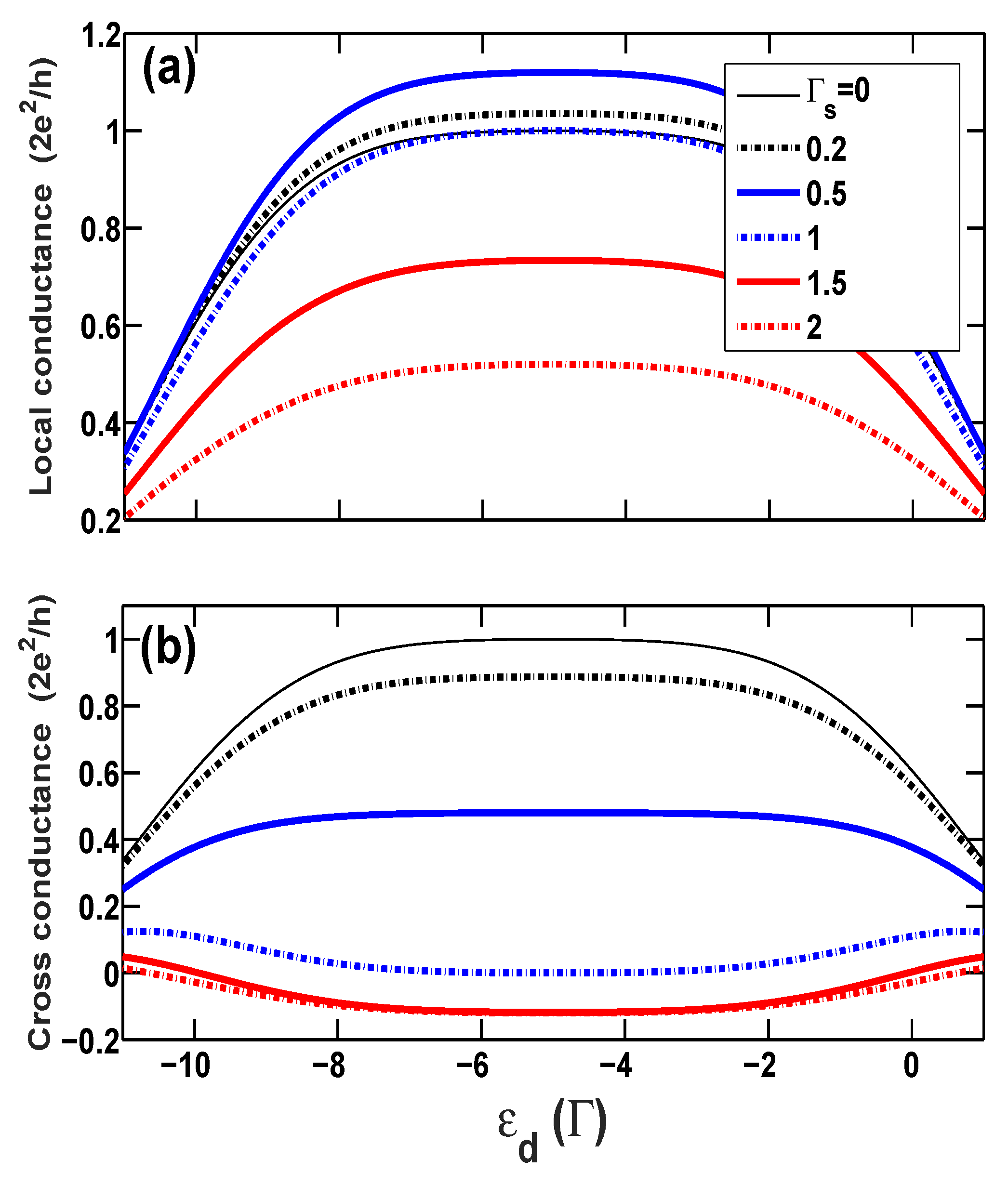
Firstly, we show the calculated linear conductances in Figure 2, including the local conductance and the nonlocal cross conductance as functions of the bare energy level of the QD at different superconducting coupling strengths, , , , , , and , in the case of no spin-polarization . Without the superconducting coupling , and the linear conductance reaches the unitary limit, (), as expected in the Kondo regime. With increasing the coupling , the local conductance raises at the beginning, as seen in Figure 2a, since the AR channel starts to emerge and contribute to the electronic tunneling. A slightly bigger value of conductance, , than the unitary limit of conductance of single-particle tunneling is reached at the coupling in the Kondo regime. On the other hand, it is known that the resonant AR leads to the unitary limit of conductance, , of the Cooper pair tunneling in the two-terminal hybrid system, e.g., a normal metal-QD-superconductor system [24]. We can therefore deduce that such a larger value of the conductance is a signature indicating that the tunneling event in the present hybrid system is a mixture of the single-particle and Cooper pair tunnelings. Increasing the coupling further will, however, cause a decrease in the local conductance . The suppression of can be interpreted as follows: An electron coming from the left lead has much higher probability to form the Cooper pair breaking into the superconducting electrode due to the considerable strength of the coupling , and as a result, the ET process is rapidly suppressed. Different from the local conductance, the nonlocal conductance decreases from the beginning and even becomes negative if the proximity-coupling is sufficiently strong. The negative cross conductance means that when the left lead is applied with a voltage which is bigger than the right lead, electrons will, instead of entering into the right lead from the QD, tunnel into the QD out of the right lead. Moreover, we find that when the QD leaves the Kondo regime, the cross conductance becomes positive again.
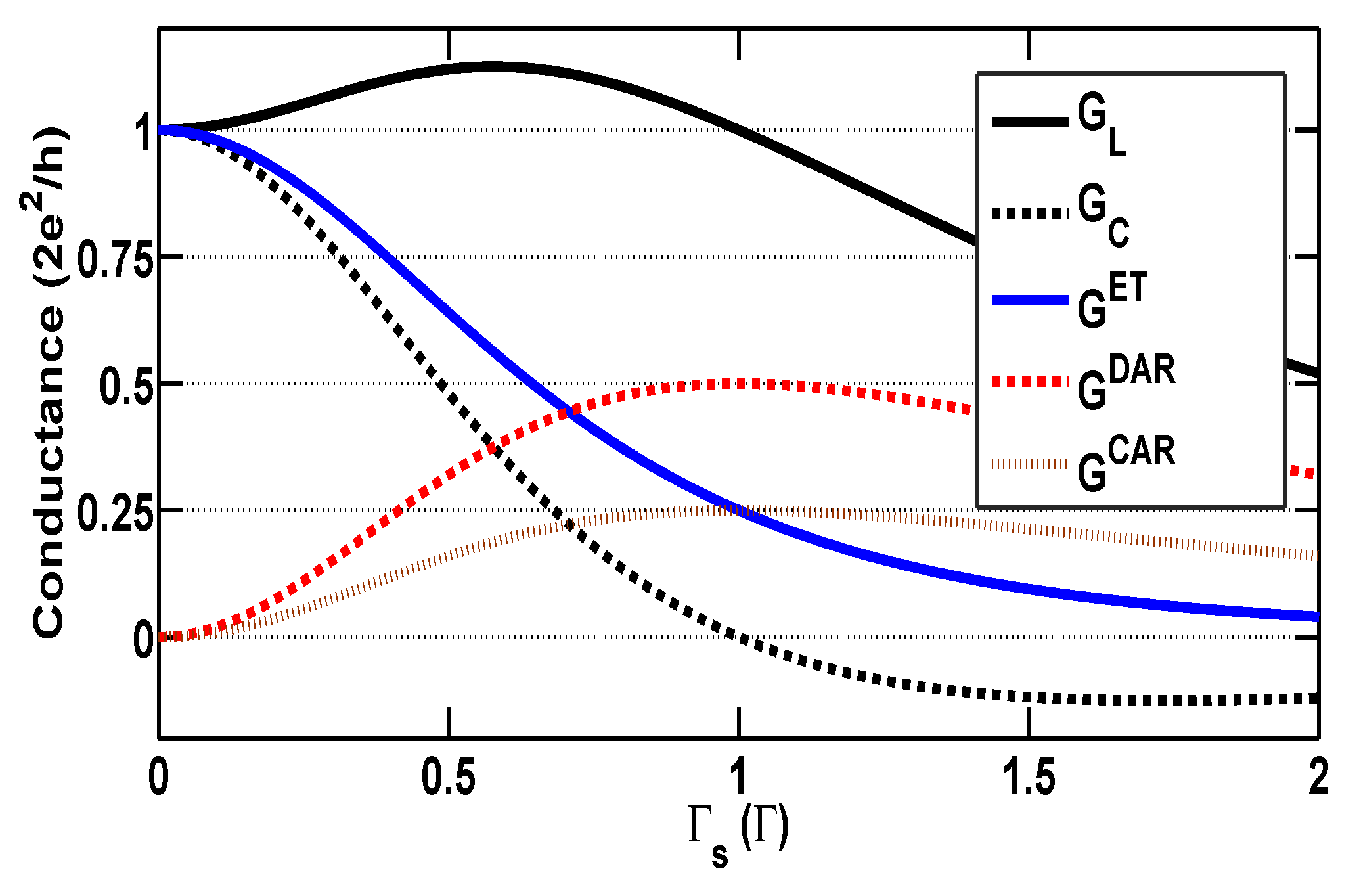
Such effects of are clearly manifested in Figure 3, in which the local and nonlocal conductances, and their three respective parts, , , and , are illustrated as functions of the coupling for the specific system which has bare dot level, . It is observed that a maximum value of the local conductance, , is arrived at, . After this point of , the AR process becomes the predominate tunneling mechanism over the ET process. When the proximity-coupling is equal to the tunnel-coupling, i.e., , a new resonance is reached, originating from interplay between the Kondo effect and AR. Consequently, and , and the local conductance arrive at the unitary value, once more. At the same time, the nonlocal conductance completely vanishes, , which indicates no current response in the right lead to the bias voltage applied to the left lead.
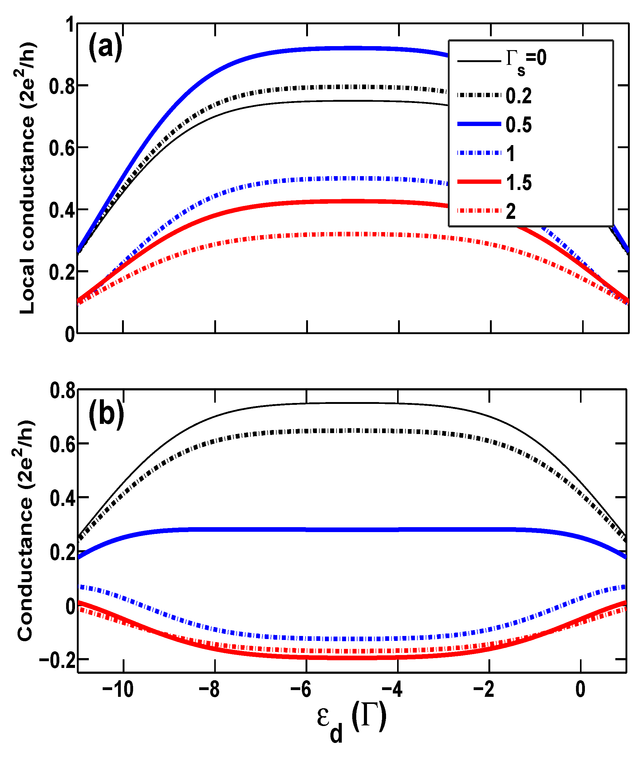
Secondly, in Figure 4, we investigate the cross conductance as a function of the bare energy level of the QD at different proximity couplings in the AP configuration with a large spin polarization . In the AP configuration, similar with the case of zero spin polarization , electrons with up-spin and down-spin are equally available in the whole system, favoring the formation of the Kondo-correlated state within a wide dot level range centered at . Meanwhile, since there is no splitting of the renormalized dot levels, , for different spins, the usual tunneling and charging peaks, around and , respectively, are relatively narrow. The local conductance vs. curves show a similar behavior as the case of zero spin polarization even in the presence of superconducting coupling . Furthermore, since no spin-flip scattering exists in the tunneling processes, in the AP configuration, the majority-spin (e.g., up-spin) states in the left lead increase but the available up-spin (minority-spin) states in the right lead decrease with increasing spin polarization strength, and as a consequence, the transfer of the majority-spin (up-spin) electrons through the QD is suppressed, such that the local conductance goes down and eventually vanishes at as expected. On the contrary, the available down-spin states in the right lead increase in the AP configuration, which just facilitates the occurrence of the CAR process [30]. Therefore, one can observe that becomes negative in almost the whole region of dot levels, from the mixed-valence regime to the empty orbital regime, even when , and nearly arrives at a considerably bigger negative value, , at the Kondo regime at . It is interesting to consider the extreme case of . As mentioned above, in the AP configuration electrons with up-spin and down-spin are identical to each other, preferring the formation of the Kondo-correlated state for all values of p. However, since the up-spin states are almost unavailable in the right lead in the case of large polarization, the ET process for the left lead to the right lead is completely damaged (implying an exactly vanishing conductance in the usual QD system), but the CAR process survives here as a unique tunneling mechanism, exclusively making a contribution to electronic tunneling. It is anticipated that in this case, and (this is the unitary limit of conductance of the single channel).
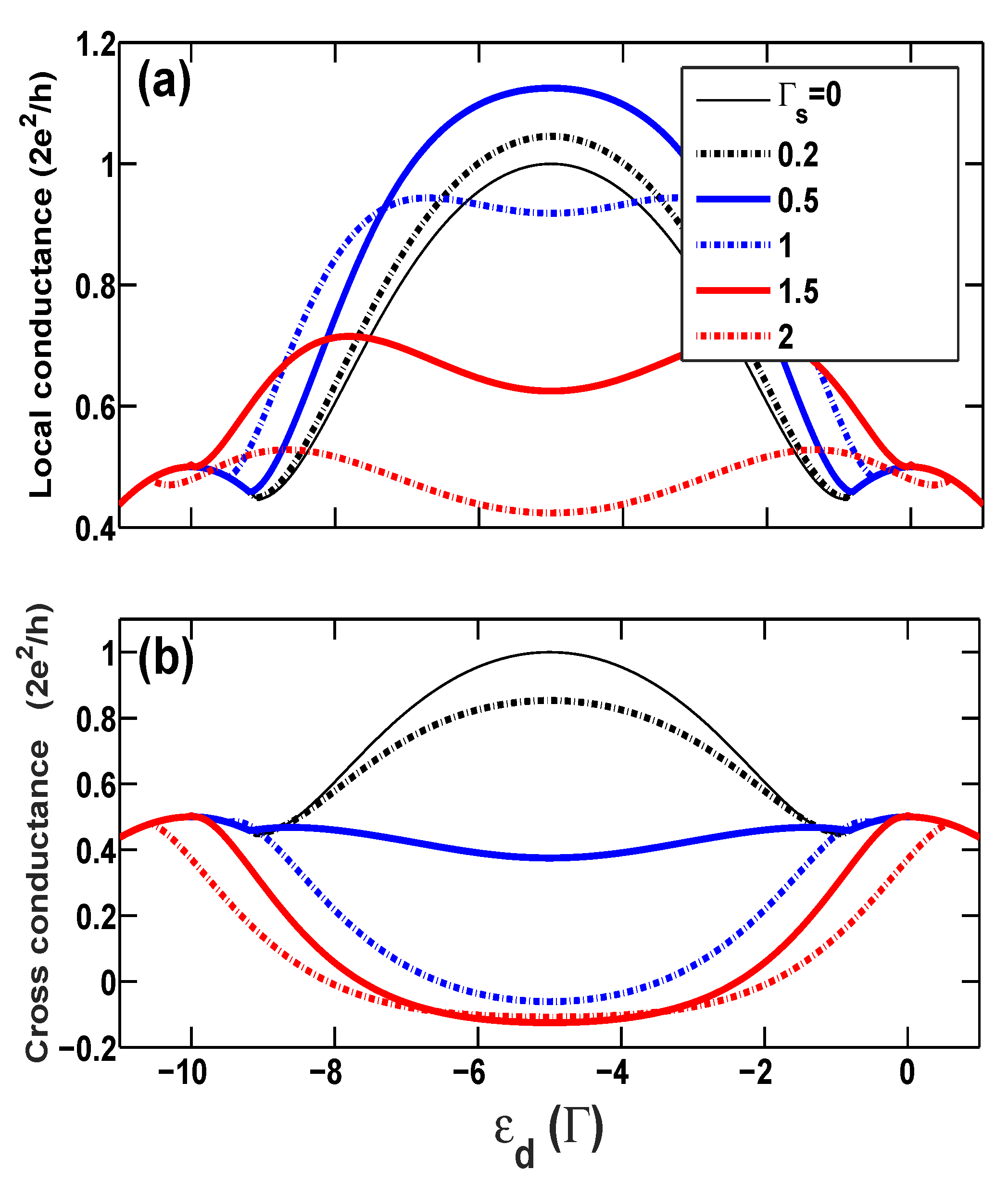
The situation is quite different in the case of the P configuration, as demonstrated in Figure 5, in which the two conductances are plotted as functions of bare dot level with spin polarization . In the P configuration, finite spin polarization splits the dot level for up- and down-spins and thus broadens the usual resonance peaks around and [32,33,34,35,36]. On one hand, since minority-spin electrons are still available in the two electrodes to build the Kondo screening correlation to a certain degree, the central Kondo peak can still be reached at the unitary limit at the large polarization in the case of . On the other hand, the number of minority-spin electrons is too small to construct the Kondo-correlated state at , and thus Kondo-induced conductance enhancement disappears rapidly when the QD moves away from the particle-hole symmetric point . These two factors cause the appearance of kinks or splitting peaks in both conductance vs. curves. Besides, it can be observed from Figure 5a that the central Kondo peak in the local conductance is progressively splitting with increasing proximity coupling in this P configuration. Furthermore, a decrease in minority-spin states in both leads in the P configuration hinders the emergence of AR processes, which leads to weakly negative cross conductance in the Kondo regime, e.g., , and even causes CAR to totally vanish, thus at the two usual resonance peaks, as shown in Figure 5b. This states that strong ferromagnetism destroys proximitized superconductivity in this three-terminal hybrid nanosystem.
3.2. Nonlinear Local and Cross Conductances
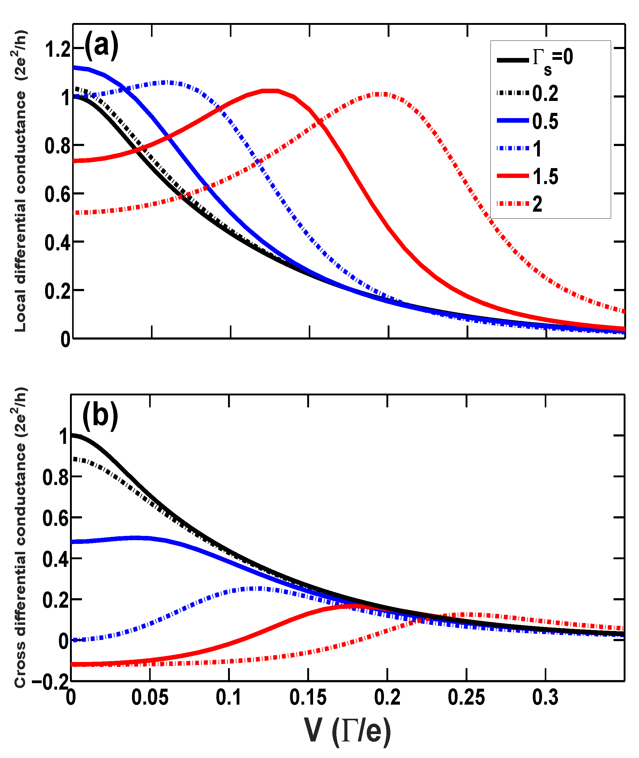
Now, we turn to the investigation of nonlinear tunneling, since the nonlinear differential conductance is believed to be a very useful tool in experiments aimed at detecting the formation of the Kondo-correlated state due to its proportionality to the transmission spectrum, supposing that the total transmission is unchanged subject to the external bias voltage. In the present three-terminal hybrid device, one can define the local and cross differential conductances, and , if the bias voltage V is applied to the left lead and while the superconducting and the right leads are kept grounded. From the Equations (26)–(29), we can obtain that the two diffenertial conductances are both proportional to the normal transmission spectrum and the AR spectrum at at zero temperature, and (a and b are constants).
Figure 6 shows the local and cross differential conductances as functions of bias voltage at various proximity couplings for the system with a single dot level () at the Kondo regime. These curves for weak proximity coupling present a single zero-bias anomaly, which is the signature of the Kondo effect. Nevertheless, there appears non-zero-bias peak with increasing proximity coupling . It is announced that the Kondo correlation enhances not only the normal ET, but also the AR; nonetheless. the increasing superconducting proximity coupling induces splitting of the Kondo peaks in the normal transmission spectrum as well as the AR spectrum. This peak splitting is the reason that the three parts of the linear conductance are all suppressed when , as shown in Figure 3. Finally, one can observe that the negative cross differential conductance becomes positive in the case of large bias voltage. External bias voltage plays a role in dissipation so as to destroy not only the Kondo correlation but the negative nonlocal current response as well.
4. Conclusions
We have theoretically investigated the subgap transport properties of a hybrid nanosystem consisting of an interacting QD connected to one superconducting lead and two ferromagnetic leads. On the basis of the finite-U slave boson mean field approach and the NGF method, we find markedly rich transport features ascribed to the competition among the Kondo correlation, superconducting proximity effect, and spin polarization of electrodes. In the case of weak superconducting proximity coupling, the Kondo-correlated state can still be built, leading to a single zero-bias peak in the voltage-dependent differential conductance. However, the peak height drops down gradually with increasing , and when , a non-zero peak appears. Such strong proximity coupling induces linear cross conductance which is negative in the Kondo region. Spin polarization can further enhance the opposite current response in the right lead (more negative cross conductance) in the AP configuration, because such a configuration is advantageous to the emergence of CAR. In contrast, in the P configuration, the rising spin polarization p blocks the CAR process and also splits the Kondo peak, such that the linear local conductance exhibits four peaks when , and the linear cross conductance reduces to the normal positive conductance more rapidly.
Author Contributions
Conceptualization, B.D.; Data curation, C.L.; Funding acquisition, B.D.; Investigation, C.L. and B.D.; Supervision, B.D. and X.-L.L.; Writing—review & editing, B.D.
Funding
National Natural Science Foundation of China: 11674223.
Acknowledgments
This work was supported by Projects of the National Science Foundation of China under Grant No. 11674223.
Conflicts of Interest
The authors declare no conflict of interest.
Appendix A
In this appendix, we briefly show how to obtain the effective Hamiltonian Equation (7). Within the formulation of the finite-U slave boson approach, the original QD electron operators are replaced by the new varibales as follows: , , and . The additional degrees of freedom simplify the Coulomb interaction as , but introduce vectors not describing physically real states. Then, two constraint conditions have to be imposed to eliminate the unphysical part of the enlarged Hilbert space
Therefore, the subspace of the enlarged Hilbert space defined by Equation (A1) is equivalent to the original Hilbert space. Applying Dirac’s formulation of constrained dynamics, one should then introduce two q-number Lagrange multipliers and , corresponding to the two constraints in Equation (A1), to the Heisenberg equation of motion with respect to the effective Hamiltonian
and consequently any dynamical observable satisfies the standard equation of motion as a state equation
The next key point of the SBMF approach is to replace all the slave-boson operators and the Lagrange multipliers by their average values according to nonequilibrium steady states (NESS), which can be still expressed in this paper by e, , d, , and . As a result, we can indeed obtain the mean-field expression of the effective Hamiltonian Equation (7) (please note that we still use the notation instead of in the effective Hamiltonian in the main text for the sake of convenience).
Appendix B
It is easily noticed that there are seven averages in total to be determined within the SBMF approach, and the constraints provide three conditions: Equations (13) and (14). Hence, four more conditions are necessary. Originally, Kotliar and Ruckenstein [46] derived them by the saddle-point approximation for the equilibrium free energy, but this approach cannot be applied in this paper, since we are dealing with the NESS. Instead, herein, we can derive those conditions from the equations of motion of the four slave boson fields according to Equation (A3). For instance, the empty boson field e obeys the equation of motion:
By replacing the slave-boson operators and Lagrange multipliers to their mean values and evaluating NESS averages of the fermionic operators, one obtains, in the condition of steady state,
Here the commutators of the boson fields are evaluated as and , according to the Dirac’s quantum algebraic scheme.
Now, we turn to discuss the averages of fermionic operators which are evaluated at a NESS with respect to the fermionic part of the effective Hamiltonian Equation (7). Since we discuss quantum transport through a nanodevice in this paper, a NESS can be defined as being when all electrodes are at equilibrium with their own temperatures and chemical potentials , and thus the statistical operator can be introduced as
In the above, is the normalization constant, and are the Hamiltonian and the total number of particles in the lead , respectively. According to the nonequilibrium statistical theory, the average of an observable with respect to such a NESS can then be evaluated as . Thereby, we can evaluate the averages of fermionic operators with the help of the NGF technique, for example, the operators of occupation number on the dot, and (Equations (15) and (16)), and the order parameter R in Equation (17). Moreover, we can define
and
Here, the hybrid NGFs, are the matrix elements of the hybrid contour-order GF matrix () with the Nambu representation in the lead . Applying the Langreth theorem, we obtain
where is the decoupled NGF of the lead defined as and
Subsequently, we have
with
Noticing the retarded and advanced self energies in the wide band limit,
and Equations (21)–(24), we can further obtain an explicit expression of Equation (A11) and insert this expression into Equations (A7) and (A8) to yield Equations (18) and (19). Finally, we obtain the self-consistent equation Equation (9).
References
- Buitelaar, M.R.; Nussbaumer, T.; Schönenberger, C. Quantum Dot in the Kondo Regime Coupled to Superconductors. Phys. Rev. Lett. 2002, 89, 256801. [Google Scholar] [CrossRef] [PubMed] [Green Version]
- Russo, S.; Kroug, M.; Klapwijk, T.M.; Morpurgo, A.F. Experimental Observation of Bias-Dependent Nonlocal Andreev Reflection. Phys. Rev. Lett. 2005, 95, 027002. [Google Scholar] [CrossRef] [PubMed]
- Cadden-Zimansky, P.; Chandrasekhar, V. Nonlocal Correlations in Normal-Metal Superconducting Systems. Phys. Rev. Lett. 2006, 97, 237003. [Google Scholar] [CrossRef] [PubMed] [Green Version]
- Jarillo-Herrero, P.; Van Dam, J.A.; Kouwenhoven, L.P. Quantum supercurrent transistors in carbon nanotubes. Nature 2006, 439, 953. [Google Scholar] [CrossRef] [PubMed]
- Van Dam, J.A.; Nazarov, Y.V.; Bakkers, E.P.; De Franceschi, S.; Kouwenhoven, L.P. Supercurrent reversal in quantum dots. Nature 2006, 442, 667. [Google Scholar] [CrossRef] [PubMed]
- Sand-Jespersen, T.; Paaske, J.; Andersen, B.M.; Grove-Rasmussen, K.; Jørgensen, H.I.; Aagesen, M.; Sørensen, C.B.; Lindelof, P.E.; Flensberg, K.; Nygård, J. Kondo-Enhanced Andreev Tunneling in InAs Nanowire Quantum Dots. Phys. Rev. Lett. 2007, 99, 126603. [Google Scholar] [CrossRef] [Green Version]
- Hofstetter, L.; Csonka, S.; Nygård, J.; Schönenberger, C. Cooper pair splitter realized in a two-quantum-dot Y-junction. Nature 2009, 461, 960. [Google Scholar] [CrossRef]
- Grove-Rasmussen, K.; Jørgensen, H.I.; Andersen, B.M.; Paaske, J.; Jespersen, T.S.; Nygård, J.; Flensberg, K.; Lindelof, P.E. Superconductivity-enhanced bias spectroscopy in carbon nanotube quantum dots. Phys. Rev. B 2009, 79, 134518. [Google Scholar] [CrossRef] [Green Version]
- Franceschi, S.D.; Kouwenhoven, L.; Schönenberger, C.; Wernsdorfer, W. Hybrid superconductor-quantum dot devices. Nat. Nanotechnol. 2010, 5, 703. [Google Scholar] [CrossRef]
- Franke, K.J.; Schulze, G.; Pascual, J.I. Competition of Superconducting Phenomena and Kondo Screening at the Nanoscale. Science 2011, 332, 940–944. Available online: https://science.sciencemag.org/content/332/6032/940.full.pdf (accessed on 11 October 2019). [CrossRef]
- Dirks, T.; Hughes, T.L.; Lal, S.; Uchoa, B.; Chen, Y.F.; Chialvo, C.; Goldbart, P.M.; Mason, N. Transport through Andreev bound states in a graphene quantum dot. Nat. Phys. 2011, 7, 386. [Google Scholar] [CrossRef]
- Schindele, J.; Baumgartner, A.; Schönenberger, C. Near-Unity Cooper Pair Splitting Efficiency. Phys. Rev. Lett. 2012, 109, 157002. [Google Scholar] [CrossRef] [PubMed]
- Braunecker, B.; Burset, P.; Levy Yeyati, A. Entanglement Detection from Conductance Measurements in Carbon Nanotube Cooper Pair Splitters. Phys. Rev. Lett. 2013, 111, 136806. [Google Scholar] [CrossRef] [PubMed]
- Lee, E.J.H.; Jiang, X.; Houzet, M.; Aguado, R.; Lieber, C.M.; Franceschi, S.D. Spin-resolved Andreev levels and parity crossings in hybrid superconductor Csemiconductor nanostructures. Nat. Nanotechnol. 2014, 9, 79. [Google Scholar] [CrossRef]
- Deacon, R.S.; Oiwa, A.; Sailer, J.; Baba, S.; Kanai, Y.; Shibata, K.; Hirakawa, K.; Tarucha, S. Cooper pair splitting in parallel quantum dot Josephson junctions. Nat. Commun. 2015, 6, 7446. [Google Scholar] [CrossRef]
- Ruby, M.; Pientka, F.; Peng, Y.; von Oppen, F.; Heinrich, B.W.; Franke, K.J. Tunneling Processes into Localized Subgap States in Superconductors. Phys. Rev. Lett. 2015, 115, 087001. [Google Scholar] [CrossRef]
- Fülöp, G.; Domínguez, F.; d’Hollosy, S.; Baumgartner, A.; Makk, P.; Madsen, M.H.; Guzenko, V.A.; Nygård, J.; Schönenberger, C.; Levy Yeyati, A.; et al. Magnetic Field Tuning and Quantum Interference in a Cooper Pair Splitter. Phys. Rev. Lett. 2015, 115, 227003. [Google Scholar] [CrossRef]
- Albrecht, S.M.; Higginbotham, A.P.; Madsen, M.; Kuemmeth, F.; Jespersen, T.S.; Nygård, J.; Krogstrup, P.; Marcus, C.M. Exponential protection of zero modes in Majorana islands. Nature 2016, 531, 206. [Google Scholar] [CrossRef]
- Ruby, M.; Peng, Y.; von Oppen, F.; Heinrich, B.W.; Franke, K.J. Orbital Picture of Yu-Shiba-Rusinov Multiplets. Phys. Rev. Lett. 2016, 117, 186801. [Google Scholar] [CrossRef]
- Lutchyn, R.M.; Sau, J.D.; Das Sarma, S. Majorana Fermions and a Topological Phase Transition in Semiconductor-Superconductor Heterostructures. Phys. Rev. Lett. 2010, 105, 077001. [Google Scholar] [CrossRef] [Green Version]
- Cuevas, J.C.; Levy Yeyati, A.; Martín-Rodero, A. Kondo effect in normal-superconductor quantum dots. Phys. Rev. B 2001, 63, 094515. [Google Scholar] [CrossRef] [Green Version]
- Eldridge, J.; Pala, M.G.; Governale, M.; König, J. Superconducting proximity effect in interacting double-dot systems. Phys. Rev. B 2010, 82, 184507. [Google Scholar] [CrossRef]
- Golubev, D.S.; Zaikin, A.D. Shot noise and Coulomb effects on nonlocal electron transport in normal-metal/superconductor/normal-metal heterostructures. Phys. Rev. B 2010, 82, 134508. [Google Scholar] [CrossRef]
- Martín-Rodero, A.; Yeyati, A.L. Josephson and Andreev transport through quantum dots. Adv. Phys. 2011, 60, 899–958. [Google Scholar] [CrossRef] [Green Version]
- Yamada, Y.; Tanaka, Y.; Kawakami, N. Interplay of Kondo and superconducting correlations in the nonequilibrium Andreev transport through a quantum dot. Phys. Rev. B 2011, 84, 075484. [Google Scholar] [CrossRef]
- Moghaddam, A.G.; Governale, M.; König, J. Driven superconducting proximity effect in interacting quantum dots. Phys. Rev. B 2012, 85, 094518. [Google Scholar] [CrossRef]
- Koga, A. Quantum Monte Carlo study of nonequilibrium transport through a quantum dot coupled to normal and superconducting leads. Phys. Rev. B 2013, 87, 115409. [Google Scholar] [CrossRef]
- Kiršanskas, G.; Goldstein, M.; Flensberg, K.; Glazman, L.I.; Paaske, J. Yu-Shiba-Rusinov states in phase-biased superconductor–quantum dot–superconductor junctions. Phys. Rev. B 2015, 92, 235422. [Google Scholar] [CrossRef]
- Žitko, R. Spectral properties of Shiba subgap states at finite temperatures. Phys. Rev. B 2016, 93, 195125. [Google Scholar] [CrossRef] [Green Version]
- Beckmann, D.; Weber, H.B.; Löhneysen, H.V. Evidence for Crossed Andreev Reflection in Superconductor-Ferromagnet Hybrid Structures. Phys. Rev. Lett. 2004, 93, 197003. [Google Scholar] [CrossRef] [Green Version]
- Hofstetter, L.; Geresdi, A.; Aagesen, M.; Nygård, J.; Schönenberger, C.; Csonka, S. Ferromagnetic Proximity Effect in a Ferromagnet–Quantum-Dot–Superconductor Device. Phys. Rev. Lett. 2010, 104, 246804. [Google Scholar] [CrossRef] [PubMed]
- Martinek, J.; Utsumi, Y.; Imamura, H.; Barnaś, J.; Maekawa, S.; König, J.; Schön, G. Kondo Effect in Quantum Dots Coupled to Ferromagnetic Leads. Phys. Rev. Lett. 2003, 91, 127203. [Google Scholar] [CrossRef] [PubMed] [Green Version]
- Pasupathy, A.N.; Bialczak, R.C.; Martinek, J.; Grose, J.E.; Donev, L.A.K.; McEuen, P.L.; Ralph, D.C. The Kondo Effect in the Presence of Ferromagnetism. Science 2004, 306, 86–89. [Google Scholar] [CrossRef] [PubMed] [Green Version]
- Hauptmann, J.R.; Paaske, J.; Lindelof, P.E. Electric-field-controlled spin reversal in a quantum dot with ferromagnetic contacts. Nat. Phys. 2008, 4, 373. [Google Scholar] [CrossRef]
- Gaass, M.; Hüttel, A.K.; Kang, K.; Weymann, I.; von Delft, J.; Strunk, C. Universality of the Kondo Effect in Quantum Dots with Ferromagnetic Leads. Phys. Rev. Lett. 2011, 107, 176808. [Google Scholar] [CrossRef] [Green Version]
- Dong, B.; Cui, H.L.; Liu, S.Y.; Lei, X.L. Kondo-type transport through an interacting quantum dot coupled to ferromagnetic leads. J. Phys.-Condes. Matter 2003, 15, 8435–8444. [Google Scholar] [CrossRef]
- Choi, M.S.; Sánchez, D.; López, R. Kondo Effect in a Quantum Dot Coupled to Ferromagnetic Leads: A Numerical Renormalization Group Analysis. Phys. Rev. Lett. 2004, 92, 056601. [Google Scholar] [CrossRef] [Green Version]
- Sánchez, D.; López, R.; Samuelsson, P.; Büttiker, M. Andreev drag effect in ferromagnetic-normal-superconducting systems. Phys. Rev. B 2003, 68, 214501. [Google Scholar] [CrossRef] [Green Version]
- Weymann, I.; Wójcik, K.P. Andreev transport in a correlated ferromagnet-quantum-dot-superconductor device. Phys. Rev. B 2015, 92, 245307. [Google Scholar] [CrossRef]
- Futterer, D.; Governale, M.; Pala, M.G.; König, J. Nonlocal Andreev transport through an interacting quantum dot. Phys. Rev. B 2009, 79, 054505. [Google Scholar] [CrossRef] [Green Version]
- Futterer, D.; Governale, M.; König, J. Generation of pure spin currents by superconducting proximity effect in quantum dots. EPL (Europhys. Lett.) 2010, 91, 47004. [Google Scholar] [CrossRef]
- Sothmann, B.; Futterer, D.; Governale, M.; König, J. Probing the exchange field of a quantum-dot spin valve by a superconducting lead. Phys. Rev. B 2010, 82, 094514. [Google Scholar] [CrossRef]
- Weymann, I.; Trocha, P. Superconducting proximity effect and zero-bias anomaly in transport through quantum dots weakly attached to ferromagnetic leads. Phys. Rev. B 2014, 89, 115305. [Google Scholar] [CrossRef]
- Michałek, G.; Bułka, B.R.; Domański, T.; Wysokiński, K.I. Interplay between direct and crossed Andreev reflections in hybrid nanostructures. Phys. Rev. B 2013, 88, 155425. [Google Scholar] [CrossRef]
- Michałek, G.; Domański, T.; Bułka, B.R.; Wysokiński, K.I. Novel non-local effects in three-terminal hybrid devices with quantum dot. Sci. Rep. 2015, 5, 14572. [Google Scholar] [CrossRef] [Green Version]
- Kotliar, G.; Ruckenstein, A.E. New Functional Integral Approach to Strongly Correlated Fermi Systems: The Gutzwiller Approximation as a Saddle Point. Phys. Rev. Lett. 1986, 57, 1362–1365. [Google Scholar] [CrossRef]
- Schönhammer, K. Variational results as saddle-point approximations: The Anderson impurity model. Phys. Rev. B 1990, 42, 2591–2593. [Google Scholar] [CrossRef]
- Aguado, R.; Langreth, D.C. Out-of-Equilibrium Kondo Effect in Double Quantum Dots. Phys. Rev. Lett. 2000, 85, 1946–1949. [Google Scholar] [CrossRef] [Green Version]
- Dong, B.; Lei, X.L. Kondo effect and antiferromagnetic correlation in transport through tunneling-coupled double quantum dots. Phys. Rev. B 2002, 65, 241304. [Google Scholar] [CrossRef] [Green Version]
- Dong, B.; Lei, X.L. Kondo-type transport through a quantum dot under magnetic fields. Phys. Rev. B 2001, 63, 235306. [Google Scholar] [CrossRef]
- Dong, B.; Lei, X.L. Kondo-type transport through a quantum dot: a new finite-Uslave-boson mean-field approach. J. Phys.-Condes. Matter 2001, 13, 9245–9258. [Google Scholar] [CrossRef]
- Ma, J.; Dong, B.; Lei, X.L. Spin-Polarized Transport Through a Quantum Dot Coupled to Ferromagnetic Leads: Kondo Correlation Effect. Commun. Theor. Phys. 2005, 43, 341–348. [Google Scholar] [CrossRef] [Green Version]
- Bergeret, F.S.; Yeyati, A.L.; Martín-Rodero, A. Interplay between Josephson effect and magnetic interactions in double quantum dots. Phys. Rev. B 2006, 74, 132505. [Google Scholar] [CrossRef] [Green Version]
Figure 1.
(Color online) Schematic diagram of a quantum dot connected to one superconducting lead and two ferromagnetic leads.
Figure 1.
(Color online) Schematic diagram of a quantum dot connected to one superconducting lead and two ferromagnetic leads.

Figure 2.
(Color online) (a) The local conductance and (b) the cross conductance vs. the bare dot level at zero temperature for different proximity-coupling strengths in the case of normal leads, i.e., .
Figure 2.
(Color online) (a) The local conductance and (b) the cross conductance vs. the bare dot level at zero temperature for different proximity-coupling strengths in the case of normal leads, i.e., .

Figure 3.
(Color online) The zero temperature local conductance (black-solid line) and the cross conductance (black-dotted line) vs. the proximity coupling for the system with a bare dot level at the particle-hole symmetric point, in the case of normal leads (). The three parts of the conductance are also plotted for illustration purposes.

Figure 4.
(Colour online) (a) The local conductance and (b) the cross conductance versus the bare dot level for different proximity-coupling strengths in the AP configuration with .
Figure 4.
(Colour online) (a) The local conductance and (b) the cross conductance versus the bare dot level for different proximity-coupling strengths in the AP configuration with .

Figure 5.
(Color online) (a) The local conductance and (b) the cross conductance vs. the bare dot level with at zero temperature for different proximity-coupling strengths in the P configuration with .
Figure 5.
(Color online) (a) The local conductance and (b) the cross conductance vs. the bare dot level with at zero temperature for different proximity-coupling strengths in the P configuration with .

Figure 6.
(Color online) The zero-temperature local (a) and cross (b) differential conductances vs. bias voltage V for various couplings for the system with bare dot level and in the case of normal leads ().
Figure 6.
(Color online) The zero-temperature local (a) and cross (b) differential conductances vs. bias voltage V for various couplings for the system with bare dot level and in the case of normal leads ().

© 2019 by the authors. Licensee MDPI, Basel, Switzerland. This article is an open access article distributed under the terms and conditions of the Creative Commons Attribution (CC BY) license (http://creativecommons.org/licenses/by/4.0/).
Share and Cite
MDPI and ACS Style
Lee, C.; Dong, B.; Lei, X.-L. Enhanced Negative Nonlocal Conductance in an Interacting Quantum Dot Connected to Two Ferromagnetic Leads and One Superconducting Lead. Entropy 2019, 21, 1003. https://doi.org/10.3390/e21101003
AMA Style
Lee C, Dong B, Lei X-L. Enhanced Negative Nonlocal Conductance in an Interacting Quantum Dot Connected to Two Ferromagnetic Leads and One Superconducting Lead. Entropy. 2019; 21(10):1003. https://doi.org/10.3390/e21101003
Chicago/Turabian StyleLee, Cong, Bing Dong, and Xiao-Lin Lei. 2019. "Enhanced Negative Nonlocal Conductance in an Interacting Quantum Dot Connected to Two Ferromagnetic Leads and One Superconducting Lead" Entropy 21, no. 10: 1003. https://doi.org/10.3390/e21101003
Note that from the first issue of 2016, this journal uses article numbers instead of page numbers. See further details here.