Entropy of the Multi-Channel EEG Recordings Identifies the Distributed Signatures of Negative, Neutral and Positive Affect in Whole-Brain Variability


Abstract
:1. Introduction
2. Results
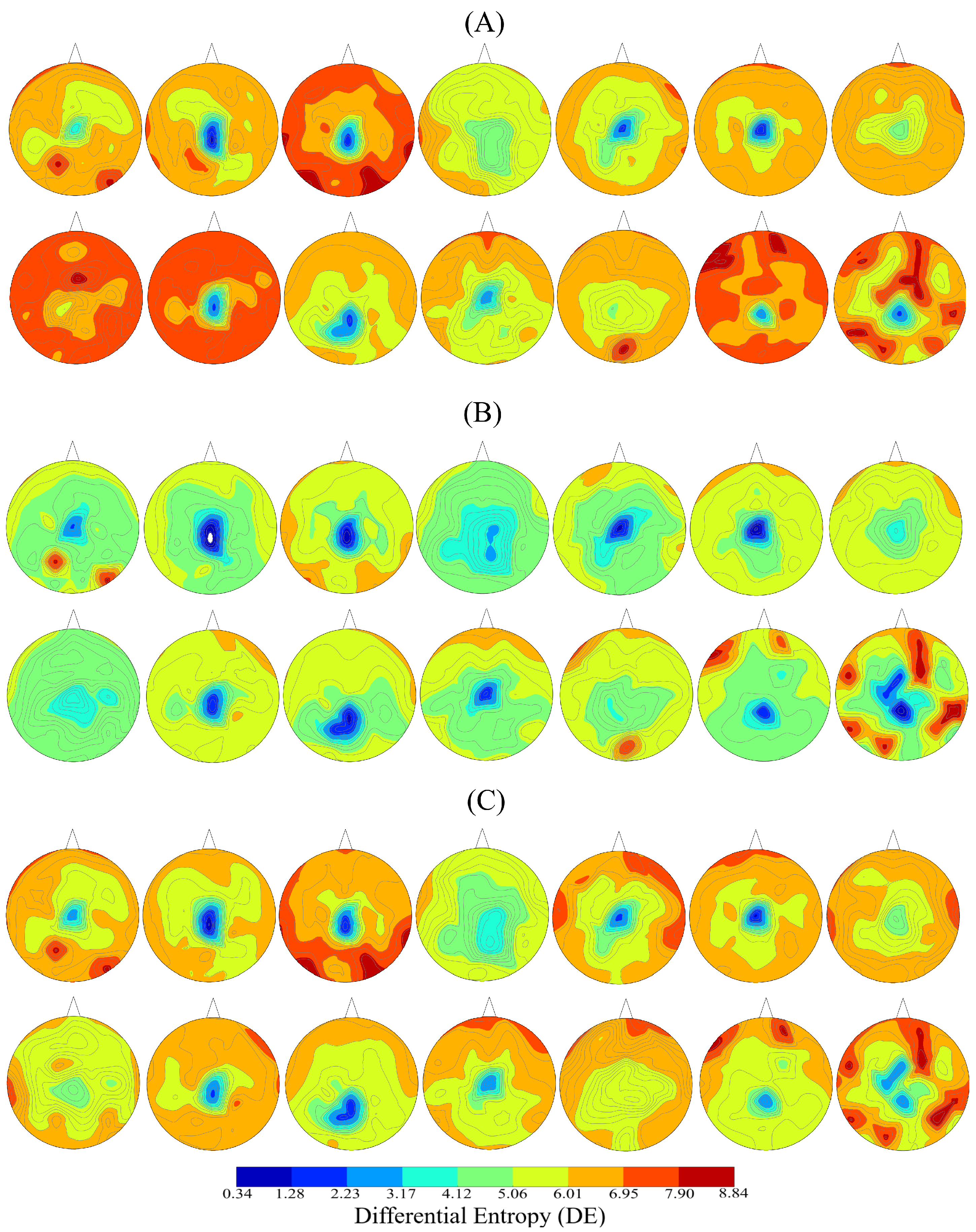
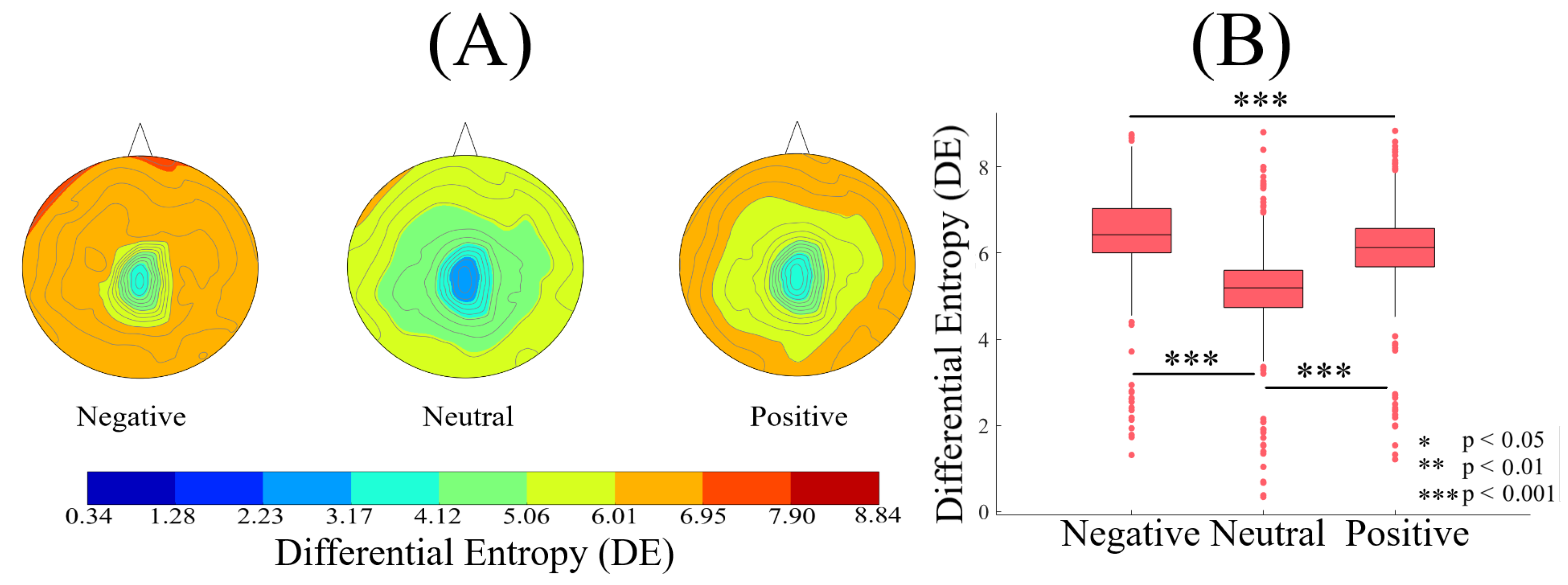
2.1. DE
2.2. The Linear Model
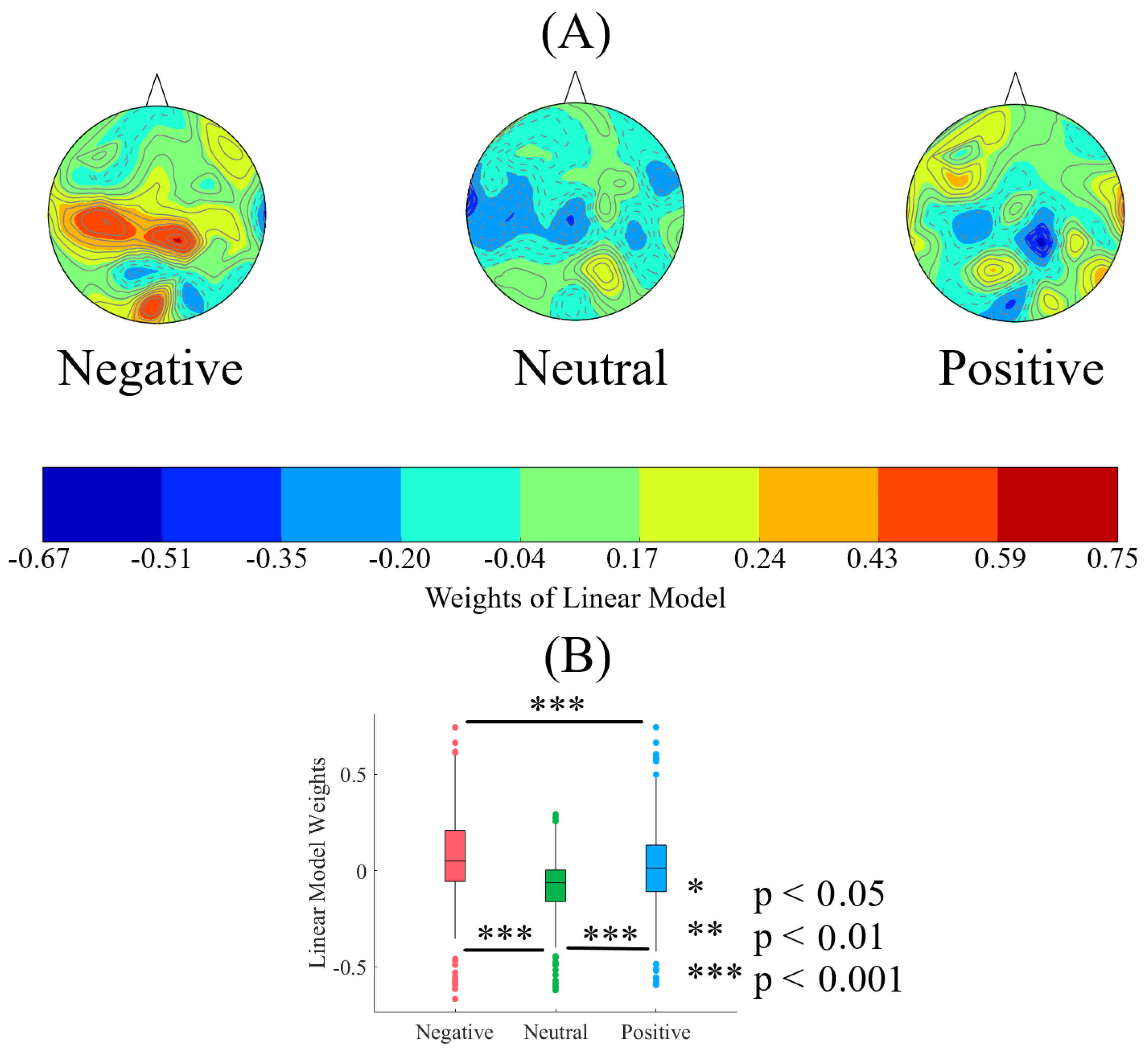
2.2.1. Weights
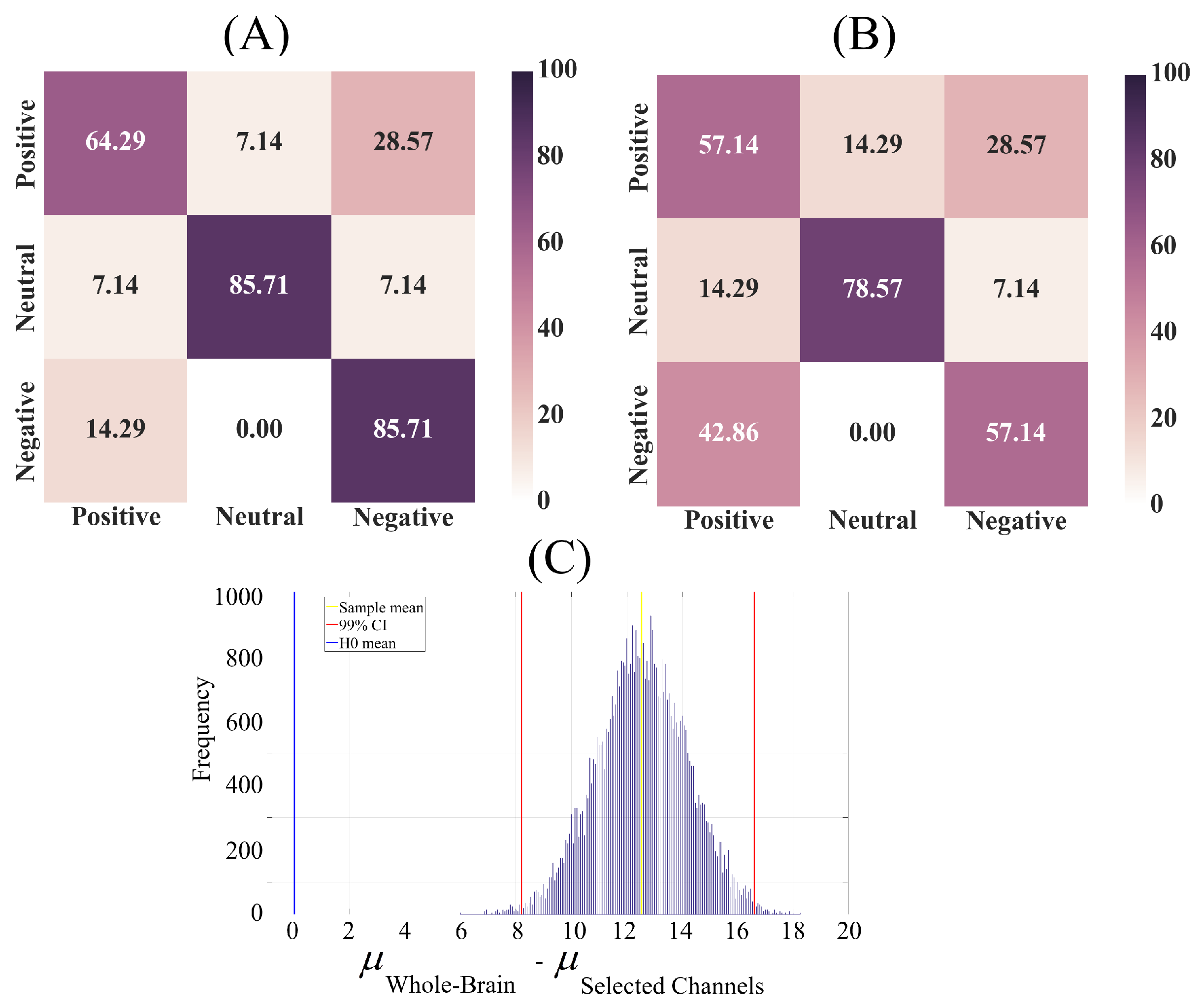
2.2.2. Affect Prediction
3. Materials and Methods
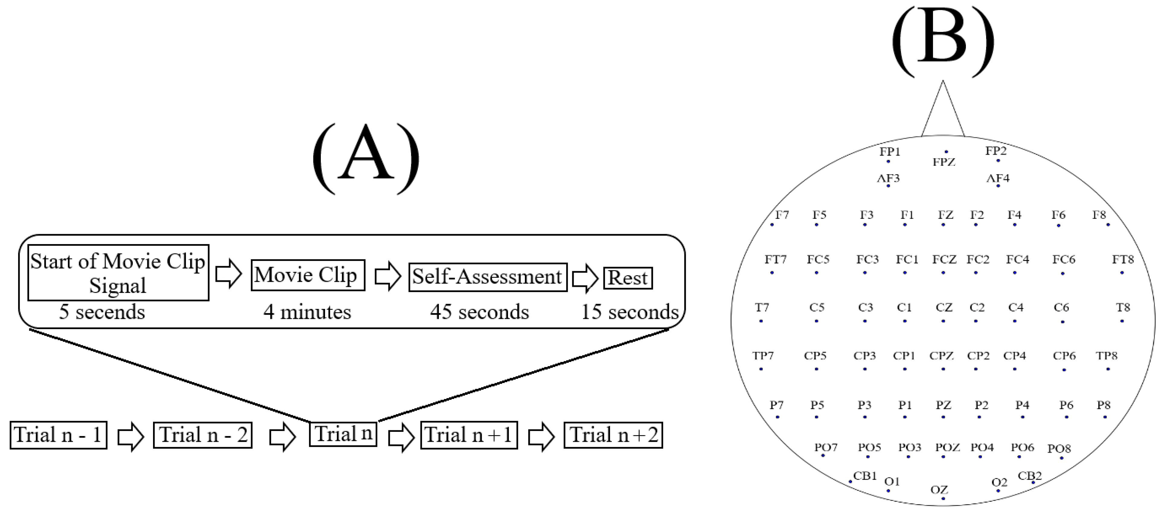
3.1. The Dataset
3.2. Data Selection and Validation
3.3. DE Computations
3.4. Statistical Analysis
3.4.1. DE Analyses
3.4.2. Linear Model Training
- Use of DEs associated with all EEG channels, thereby considering the whole-brain variability. This resulted in the linear model’s input feature vectors that were of length sixty-two, per participant, per affect.
- Feature vectors whose DE entires were associated with the subset of EEG channels that yielded the same pattern of significant difference as in the case of whole-brain comparison (i.e., the second step in DE analyses, Appendix A).
4. Discussion
5. Limitations and Future Direction
Author Contributions
Funding
Conflicts of Interest
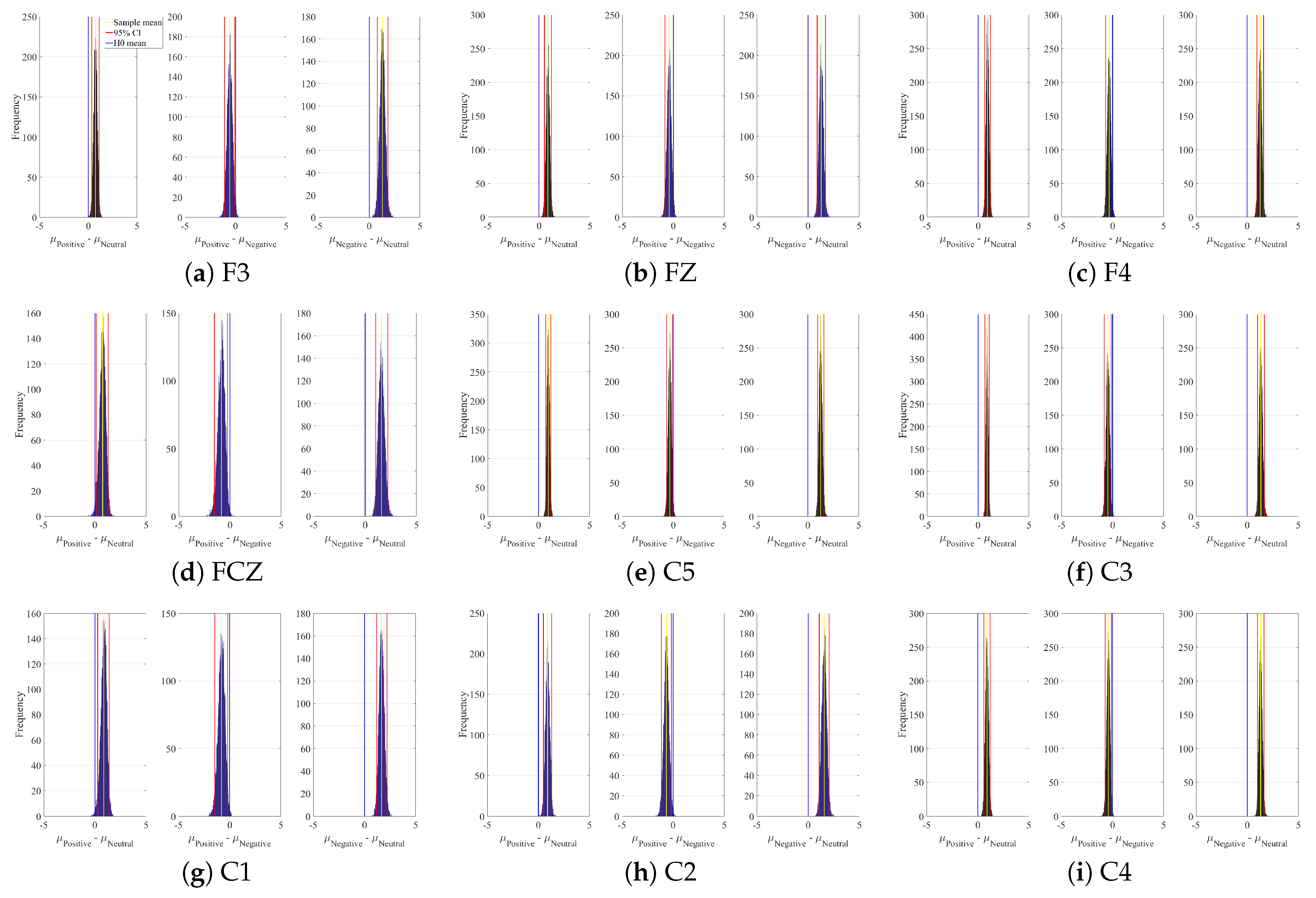
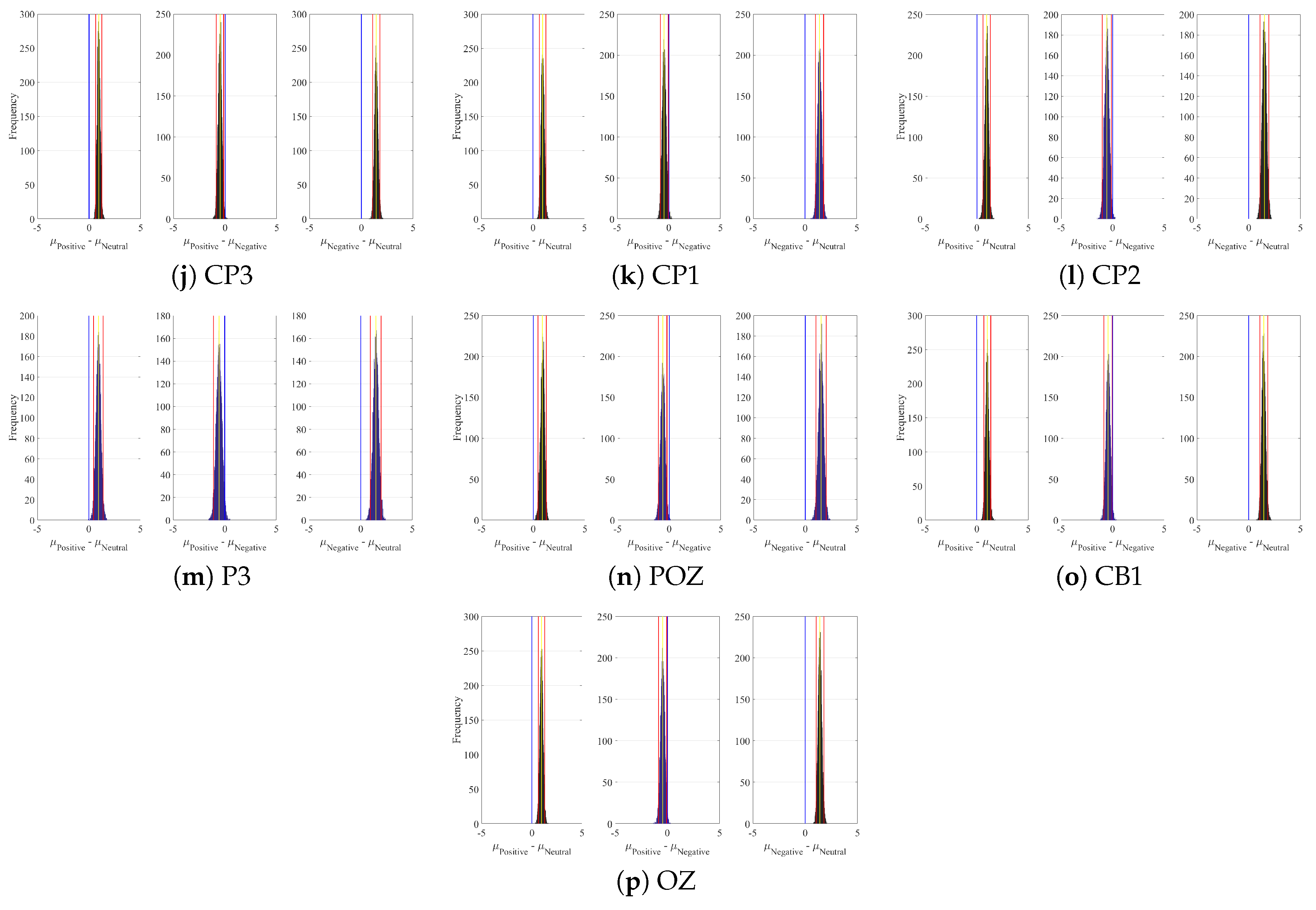
Appendix A. Channels with Significant DE Differences


| Channel | Conditions | M | SD | 95.0% CI |
|---|---|---|---|---|
| Positive versus Neutral | 0.74 | 0.19 | [0.36 1.10] | |
| F3 | Positive versus Negative | 0.26 | [ ] | |
| Negative versus Neutral | 1.32 | 0.26 | [0.80 1.84] | |
| Positive versus Neutral | 0.88 | 0.18 | [0.53 1.22] | |
| FZ | Positive versus Negative | 0.21 | [ ] | |
| Negative versus Neutral | 1.29 | 0.20 | [0.90 1.69] | |
| Positive versus Neutral | 0.92 | 0.14 | [0.64 1.20] | |
| F4 | Positive versus Negative | 0.17 | [ ] | |
| Negative versus Neutral | 1.26 | 0.17 | [0.94 1.60] | |
| Positive versus Neutral | 0.75 | 0.29 | [0.14 1.29] | |
| FCZ | Positive versus Negative | 0.33 | [] | |
| Negative versus Neutral | 1.59 | 0.29 | [1.03 2.18] | |
| Positive versus Neutral | 0.75 | 0.94 | [0.69 1.19] | |
| C5 | Positive versus Negative | 0.16 | [] | |
| Negative versus Neutral | 1.27 | 0.16 | [0.97 1.58] | |
| Positive versus Neutral | 0.89 | 0.11 | [0.68 1.10] | |
| C3 | Positive versus Negative | 0.17 | [] | |
| Negative versus Neutral | 1.35 | 0.17 | [1.02 1.68] | |
| Positive versus Neutral | 0.87 | 0.28 | [0.29 1.38] | |
| C1 | Positive versus Negative | 1 | 0.31 | [] |
| Negative versus Neutral | 1.67 | 0.26 | [1.18 2.19] | |
| Positive versus Neutral | 0.89 | 0.20 | [0.48 1.28] | |
| C2 | Positive versus Negative | 0.25 | [] | |
| Negative versus Neutral | 1.56 | 0.25 | [1.07 2.03] | |
| Positive versus Neutral | 0.91 | 0.15 | [0.60 1.20] | |
| C4 | Positive versus Negative | 0.16 | [] | |
| Negative versus Neutral | 1.30 | 0.16 | [0.99 1.62] | |
| Positive versus Neutral | 0.94 | 0.15 | [0.66 1.24] | |
| CP3 | Positive versus Negative | 0.18 | [] | |
| Negative versus Neutral | 1.44 | 0.17 | [1.11 1.78] | |
| Positive versus Neutral | 0.95 | 0.16 | [0.63 1.27] | |
| CP1 | Positive versus Negative | 0.19 | [] | |
| Negative versus Neutral | 1.41 | 0.20 | [1.00 1.79] | |
| Positive versus Neutral | 0.95 | 0.18 | [0.58 1.29] | |
| CP2 | Positive versus Negative | 0.23 | [] | |
| Negative versus Neutral | 1.51 | 0.21 | [1.09 1.93] | |
| Positive versus Neutral | 0.92 | 0.24 | [0.44 1.40] | |
| P3 | Positive versus Negative | 0.28 | [] | |
| Negative versus Neutral | 1.46 | 0.26 | [0.95 1.99] | |
| Positive versus Neutral | 0.88 | 0.20 | [0.45 1.25] | |
| POZ | Positive versus Negative | 0.22 | [] | |
| Negative versus Neutral | 1.52 | 0.25 | [1.01 2.01] | |
| Positive versus Neutral | 1.01 | 0.17 | [0.69 1.37] | |
| CB1 | Positive versus Negative | 0.21 | [] | |
| Negative versus Neutral | 1.45 | 0.19 | [1.09 1.84] | |
| Positive versus Neutral | 0.96 | 0.16 | [0.64 1.28] | |
| OZ | Positive versus Negative | 0.20 | [] | |
| Negative versus Neutral | 1.41 | 0.19 | [1.06 1.78] |
| M | SD | CI | M | SD | CI | M | SD | CI | |
|---|---|---|---|---|---|---|---|---|---|
| F3 | 6.69 | 0.87 | [6.27 7.10] | 5.37 | 0.54 | [5.11 5.63] | 6.11 | 0.50 | [5.87 6.35] |
| FZ | 6.37 | 0.64 | [6.07 6.68] | 5.08 | 0.48 | [4.86 5.31] | 5.96 | 0.49 | [5.73 6.19] |
| F4 | 6.41 | 0.53 | [6.16 6.66] | 5.14 | 0.39 | [4.96 5.32] | 6.07 | 0.40 | [5.87 6.26] |
| FCZ | 6.14 | 0.92 | [5.70 6.58] | 4.55 | 0.69 | [4.23 4.88] | 5.31 | 0.90 | [4.88 5.74] |
| C5 | 6.61 | 0.50 | [6.37 6.85] | 5.34 | 0.34 | [5.18 5.51] | 6.28 | 0.35 | [6.12 6.45] |
| C3 | 6.18 | 0.59 | [5.90 6.46] | 4.83 | 0.28 | [4.70 4.96] | 5.72 | 0.31 | [5.57 5.87] |
| C1 | 6.11 | 0.81 | [5.73 6.50] | 4.44 | 0.58 | [4.17 4.72] | 5.31 | 0.92 | [4.88 5.75] |
| C2 | 5.94 | 0.78 | [5.57 6.31] | 4.38 | 0.55 | [4.12 4.64] | 5.27 | 0.57 | [5.00 5.54] |
| C4 | 6.13 | 0.45 | [5.92 6.34] | 4.82 | 0.43 | [4.62 5.02] | 5.72 | 0.44 | [5.52 5.93] |
| CP3 | 6.10 | 0.56 | [5.84 6.37] | 4.66 | 0.37 | [4.49 4.84] | 5.61 | 0.45 | [5.34 5.82] |
| CP1 | 5.70 | 0.63 | [5.41 6.00] | 4.30 | 0.46 | [4.08 4.52] | 5.25 | 0.43 | [5.04 5.45] |
| CP2 | 5.95 | 0.70 | [5.62 6.28] | 4.43 | 0.47 | [4.21 4.66] | 5.38 | 0.54 | [5.13 5.64] |
| P3 | 6.45 | 0.82 | [6.06 6.84] | 4.99 | 0.64 | [4.68 5.29] | 5.91 | 0.69 | [5.58 6.24] |
| POZ | 6.56 | 0.72 | [6.22 6.90] | 5.05 | 0.66 | [4.73 5.36] | 5.93 | 0.43 | [5.72 6.13] |
| CB1 | 6.70 | 0.62 | [6.41 7.00] | 5.25 | 0.42 | [5.05 5.45] | 6.27 | 0.53 | [6.02 6.52] |
| OZ | 6.57 | 0.59 | [6.29 6.85] | 5.16 | 0.40 | [4.97 5.35] | 6.12 | 0.50 | [5.88 6.36] |
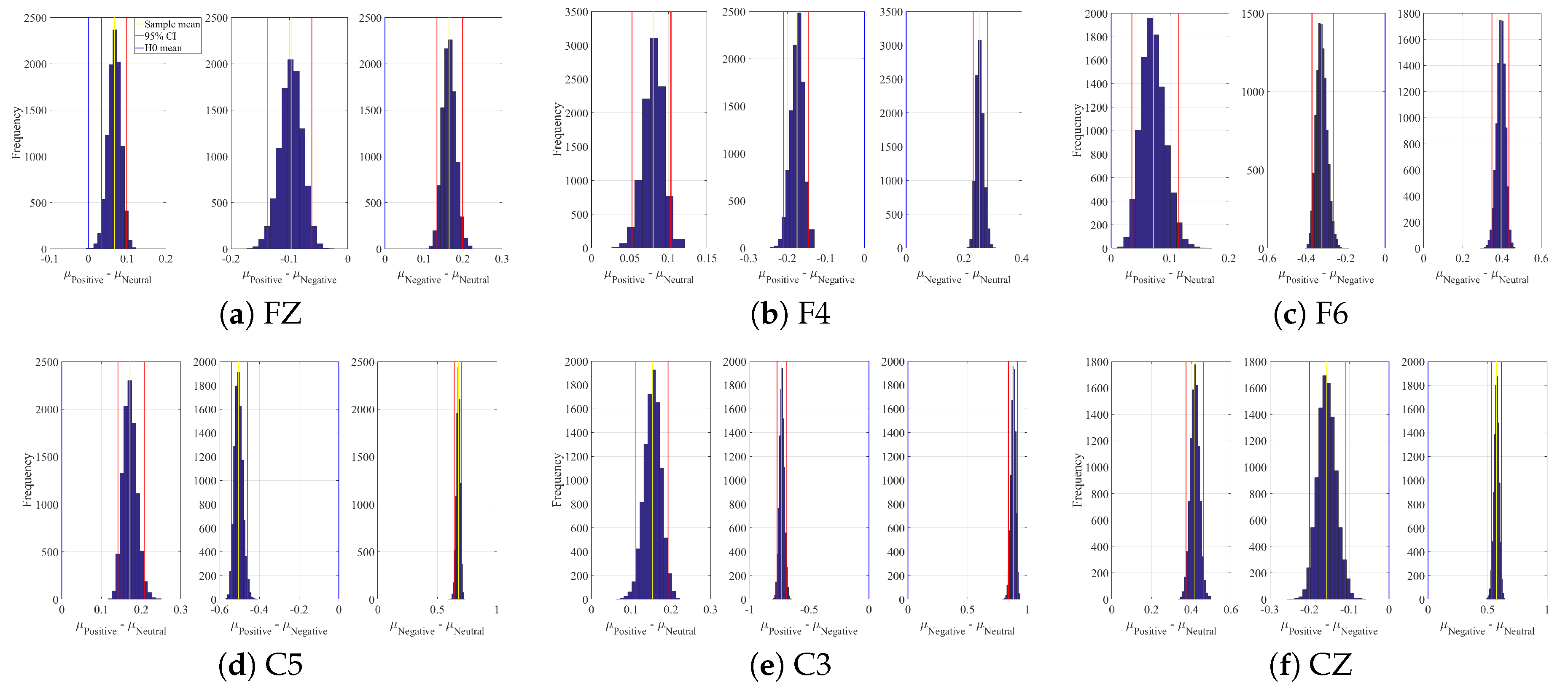
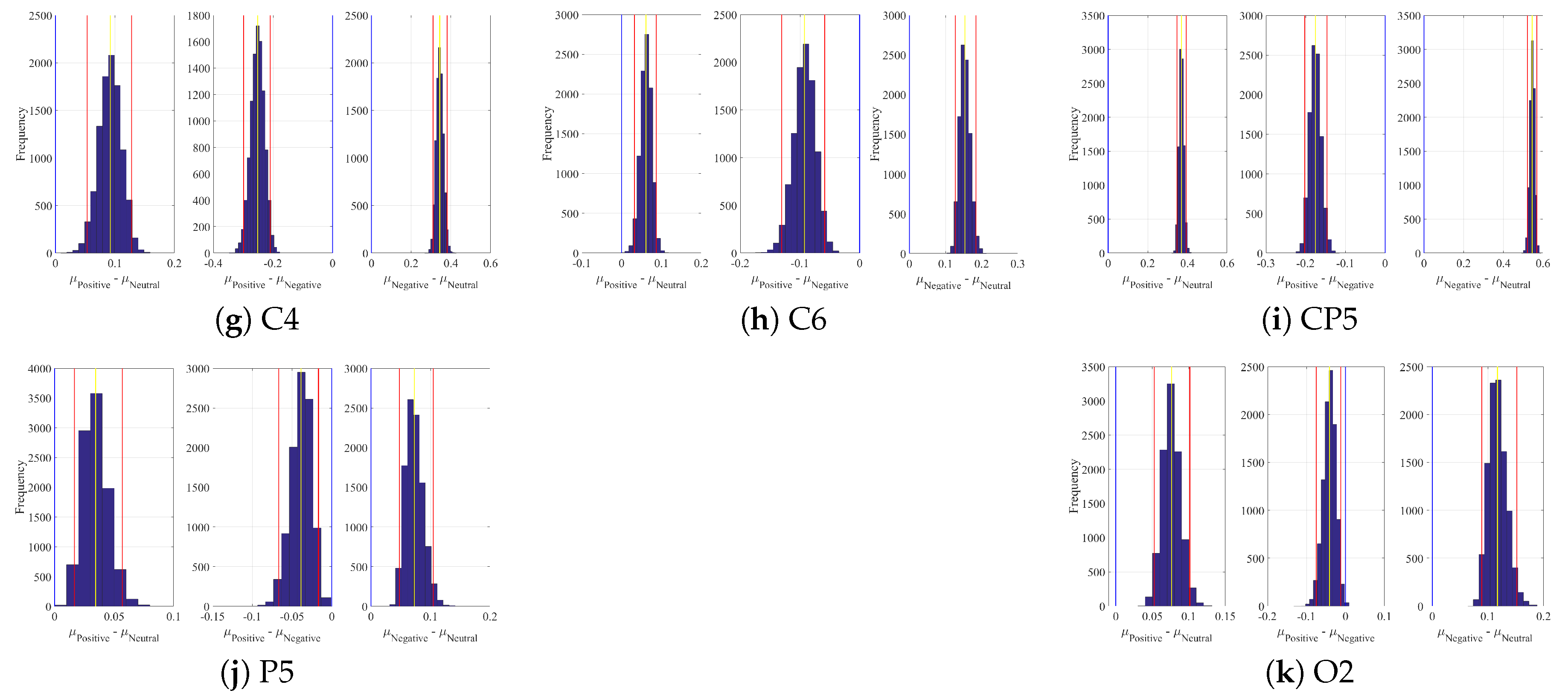
Appendix B. Linear Model’s Weights


| Channel | Conditions | M | SD | 95.0% CI |
|---|---|---|---|---|
| Negative versus Positive | 0.10 | 0.02 | [0.06 0.14] | |
| FZ | Positive versus Neutral | 0.07 | 0.02 | [0.03 0.10] |
| Negative versus Neutral | 0.16 | 0.02 | [0.13 0.20] | |
| Negative versus Positive | 0.18 | 0.02 | [0.15 0.21] | |
| F4 | Positive versus Neutral | 0.08 | 0.01 | [0.05 0.10] |
| Negative versus Neutral | 0.25 | 0.01 | [0.23 0.28] | |
| Negative versus Positive | 0.32 | 0.03 | [0.26 0.37] | |
| F6 | Positive versus Neutral | 0.07 | 0.02 | [0.03 0.11] |
| Negative versus Neutral | 0.39 | 0.02 | [0.35 0.43] | |
| Negative versus Positive | 0.50 | 0.02 | [0.46 0.54] | |
| C5 | Positive versus Neutral | 0.17 | 0.02 | [0.14 0.21] |
| Negative versus Neutral | 0.68 | 0.02 | [0.64 0.71] | |
| Negative versus Positive | 0.73 | 0.02 | [0.69 0.77] | |
| C3 | Positive versus Neutral | 0.15 | 0.02 | [0.11 0.19] |
| Negative versus Neutral | 0.88 | 0.02 | [0.84 0.92] | |
| Negative versus Positive | 0.16 | 0.02 | [0.11 0.20] | |
| CZ | Positive versus Neutral | 0.42 | 0.02 | [0.38 0.46] |
| Negative versus Neutral | 0.58 | 0.02 | [0.53 0.62] | |
| Negative versus Positive | 0.25 | 0.02 | [0.21 0.30] | |
| C4 | Positive versus Neutral | 0.09 | 0.02 | [0.05 0.13] |
| Negative versus Neutral | 0.34 | 0.02 | [0.31 0.38] | |
| Negative versus Positive | 0.09 | 0.02 | [0.06 0.13] | |
| C6 | Positive versus Neutral | 0.06 | 0.01 | [0.03 0.09] |
| Negative versus Neutral | 0.15 | 0.01 | [0.13 0.18] | |
| Negative versus Positive | 0.18 | 0.01 | [0.15 0.20] | |
| CP5 | Positive versus Neutral | 0.37 | 0.01 | [0.35 0.39] |
| Negative versus Neutral | 0.55 | 0.01 | [0.52 0.57] | |
| Negative versus Positive | 0.4 | 0.01 | [0.02 0.07] | |
| P5 | Positive versus Neutral | 0.03 | 0.01 | [0.02 0.06] |
| Negative versus Neutral | 0.07 | 0.01 | [0.05 0.11] | |
| Negative versus Positive | 0.04 | 0.02 | [0.01 0.07] | |
| O2 | Positive versus Neutral | 0.08 | 0.01 | [0.05 0.10] |
| Negative versus Neutral | 0.12 | 0.02 | [0.09 0.15] |
Appendix C. Linear Model’s Prediction—Randomized Case

| Setting | Precision | Recall | F1-Score |
|---|---|---|---|
| Whole-Brain | 0.86 | 0.71 | 0.77 |
| Selected Channels | 0.60 | 0.59 | 0.60 |
References
- Haxby, J.V.; Gobbini, M.I.; Furey, M.L.; Ishai, A.; Schouten, I.L.; Pietrini, P. Distributed and overlapping representations of faces and objects in ventral temporal cortex. Science 2001, 293, 2425–2430. [Google Scholar] [CrossRef] [PubMed] [Green Version]
- Cox, D.D.; Savoy, R. fMRI Brain Reading: Detecting and classifying distributed patterns of fMRI activity in human visual cortex. NeuroImage 2003, 19, 261–270. [Google Scholar] [CrossRef]
- Mitchell, T.M.; Hutchinson, R.; Niculescu, R.S.; Pereira, F.; Wang, X.; Just, M.; Newman, S. Learning to decode cognitive states from brain images. Mach. Learn. 2004, 57, 145–175. [Google Scholar] [CrossRef] [Green Version]
- Horikawa, T.; Tamaki, M.; Miyawaki, Y.; Kamitani, Y. Neural decoding of visual imagery during sleep. Science 2013, 340, 639–642. [Google Scholar] [CrossRef] [Green Version]
- Watson, D.; Tellegen, A. Toward a consensual structure of mood. Psychol. Bullet. 1985, 98, 219–235. [Google Scholar] [CrossRef]
- Barrett, F.L.; Russell, J.A. Independence and bipolarity in the structure of current affect. J. Personal. Soc. Psychol. 1998, 74, 967–984. [Google Scholar] [CrossRef]
- Bradley, M.M.; Codispoti, M.; Cuthbert, B.N.; Lang, P.J. Emotion and motivation I: Defensive and appetitive reactions in picture processing. Emotion 2001, 1, 276–298. [Google Scholar] [CrossRef]
- Barrett, L.F.; Bliss-Moreau, E. Affect as a psychological primitive. Adv. Exp. Soc. Psychol. 2009, 41, 167–218. [Google Scholar]
- Lewis, M. The emergence of human emotions. In Handbook of Emotions, 2nd ed.; Lewis, M., Haviland-Jones, J.M., Eds.; Guilford: New York, NY, USA, 1993; pp. 253–322. [Google Scholar]
- Farroni, T.; Menon, E.; Rigato, S.; Johnson, M.H. The perception of facial expressions in newborns. Eur. J. Dev. Psychol. 2007, 4, 2–13. [Google Scholar] [CrossRef] [Green Version]
- Osgood, C.E. The nature and measurement of meaning. Psychol. Bullet. 1952, 49, 197–237. [Google Scholar] [CrossRef] [Green Version]
- Wierzbicka, A. Semantics, Culture, and Cognition: Universal Human Concepts in Culture-Specific Configurations; Oxford University Press: Oxford, UK, 1992. [Google Scholar]
- Wundt, W. Outlines of Psychology; Thoemmes Press: Bristol, UK, 1897. [Google Scholar]
- Cacioppo, J.T.; Gardner, W.L.; Berntson, G.G. The affect system has parallel and integrative processing components: Form follows function. J. Personal. Social Psychol. 1999, 76, 839–855. [Google Scholar] [CrossRef]
- Norris, C.J.; Gollan, J.; Berntson, G.G.; Cacioppo, J.T. The current status of research on the structure of evaluative space. Biolog. Psychol. 2010, 84, 422–436. [Google Scholar] [CrossRef] [PubMed] [Green Version]
- Larsen, J.T.; McGraw, A.P.; Cacioppo, J.T. Can people feel happy and sad at the same time? J. Personal. Soc. Psychol. 2001, 81, 684–696. [Google Scholar] [CrossRef]
- Larsen, R.J.; Diener, E. Promises and Problems with the Circumplex Model of Emotion; Sage: Newbury Park, CA, USA, 1992; pp. 25–59. [Google Scholar]
- Carroll, J.M.; Yik, M.S.; Russell, J.A.; Barrett, L.F. On the psychometric principles of affect. Rev. General Psychol. 1999, 3, 14–22. [Google Scholar] [CrossRef]
- Salzman, C.D.; Fusi, S. Emotion, cognition, and mental state representation in amygdala and prefrontal cortex. Ann. Rev. Neurosci. 2010, 33, 173–202. [Google Scholar] [CrossRef] [Green Version]
- Vytal, K.; Hamann, S. Neuroimaging support for discrete neural correlates of basic emotions: A voxel-based meta-analysis. J. Cognit. Neurosci. 2010, 22, 2864–2885. [Google Scholar] [CrossRef] [Green Version]
- Kober, H.; Barrett, L.F.; Joseph, J.; Bliss-Moreau, E.; Lindquist, K.; Wager, T.D. Functional grouping and cortical/subcortical interactions in emotion: A meta-analysis of neuroimaging studies. Neuroimage 2008, 42, 998–1031. [Google Scholar] [CrossRef] [Green Version]
- Murphy, F.C.; Nimmo-Smith, I.A.N.; Lawrence, A.D. Functional neuroanatomy of emotions: A meta-analysis. Cognit. Affect. Behav. Neurosci. 2003, 3, 207–233. [Google Scholar] [CrossRef]
- Wager, T.D.; Phan, K.L.; Liberzon, I.; Taylor, S.F. Valence, gender, and lateralization of functional brain anatomy in emotion: A meta-analysis of findings from neuroimaging. Neuroimage 2003, 19, 513–531. [Google Scholar] [CrossRef]
- Kringelbach, M.L.; Rolls, E.T. The functional neuroanatomy of the human orbitofrontal cortex: Evidence from neuroimaging and neuropsychology. Progress Neurobiol. 2004, 72, 341–372. [Google Scholar] [CrossRef]
- Lindquist, K.A.; Satpute, A.B.; Wager, T.D.; Weber, J.; Barrett, L.F. The brain basis of positive and negative affect: Evidence from a meta-analysis of the human neuroimaging literature. Cereb. Cortex 2015, 26, 1910–1922. [Google Scholar] [CrossRef] [PubMed] [Green Version]
- Grimm, S.; Schmidt, C.F.; Bermpohl, F.; Heinzel, A.; Dahlem, Y.; Wyss, M.; Hell, D.; Boesiger, P.; Boeker, H.; Northoff, G. Segregated neural representation of distinct emotion dimensions in the prefrontal cortex - an fMRI study. Neuroimage 2006, 30, 325–340. [Google Scholar] [CrossRef] [PubMed]
- Kensinger, E.A.; Corkin, S. Two routes to emotional memory: Distinct neural processes for valence and arousal. Proc. Natl. Acad. Sci. USA 2004, 101, 3310–3315. [Google Scholar] [CrossRef] [PubMed] [Green Version]
- Lewis, P.A.; Gritchley, H.D.; Rotshtein, P.; Dolan, R.J. Neural correlates of processing valence and arousal in affective words. Cereb. Cortex 2007, 17, 742–748. [Google Scholar] [CrossRef] [Green Version]
- Posner, J.; Russell, J.; Gerber, A.; Gorman, D.; Colibazzi, T.; Yu, S.; Wang, Z.; Kangarlu, A.; Zhu, H.; Peterson, B.S. The neurophysiological bases of emotion: An fMRI study of the affective circumplex using emotion-denoting words. Hum. Brain Map. 2009, 30, 883–895. [Google Scholar] [CrossRef] [Green Version]
- Wutz, A.; Loonis, R.; Roy, J.E.; Donoghue, J.A.; Miller, E.K. Different levels of category abstraction by different dynamics in different prefrontal areas. Neuron 2018, 97, 1–11. [Google Scholar] [CrossRef]
- Jamieson, G.A.; Burgess, A.P. Hypnotic induction is followed by state-like changes in the organization of EEG functional connectivity in the theta and beta frequency bands in high-hypnotically susceptible individuals. Front. Hum. Neurosci. 2014, 8. [Google Scholar] [CrossRef] [Green Version]
- Garrett, D.D.; Kovacevic, N.; McIntosh, A.R.; Grady, C.L. The importance of being variable. J. Neurosci. 2011, 31, 4496–4503. [Google Scholar] [CrossRef] [Green Version]
- Heisz, J.J.; Shedden, J.M.; McIntosh, A.R. Relating brain signal variability to knowledge representation. Neuroimage 2012, 63, 1384–1392. [Google Scholar] [CrossRef]
- Garrett, D.D.; Samanez-Larkin, G.R.; MacDonald, S.W.; Lindenberger, U.; McIntosh, A.R.; Grady, C.L. Moment-to-moment brain signal variability: A next frontier in human brain mapping? Neurosci. Biobehav. Rev. 2013, 37, 610–624. [Google Scholar] [CrossRef] [Green Version]
- Pouget, A.; Drugowitsch, J.; Kepecs, A. Confidence and certainty: Distinct probabilistic quantities for different goals. Nat. Neurosci. 2016, 19, 366–374. [Google Scholar] [CrossRef] [PubMed] [Green Version]
- Friston, K. The free-energy principle: A unified brain theory? Nat. Rev. Neurosci. 2010, 11, 127–138. [Google Scholar] [CrossRef] [PubMed]
- Stein, R.B.; Gossen, E.R.; Jones, K.E. Neuronal variability: Noise or part of the signal? Nat. Rev. Neurosci. 2005, 6, 389–397. [Google Scholar] [CrossRef] [PubMed]
- Faisal, A.A.; Selen, L.P.; Wolpert, D.M. Noise in the nervous system. Nat. Rev. Neurosci. 2008, 9, 292–303. [Google Scholar] [CrossRef] [PubMed]
- Avena-Koenigsberger, A.; Misic, B.; Sporns, O. Communication dynamics in complex brain networks. Nat. Rev. Neurosci. 2018, 19, 17–33. [Google Scholar] [CrossRef] [PubMed]
- Muller, L.; Chavane, F.; Reynolds, J.; Sejnowski, T.J. Cortical travelling waves: Mechanisms and computational principles. Nat. Rev. Neurosci. 2018, 19, 255–268. [Google Scholar] [CrossRef]
- Bak, P.; Tang, C.; Wiesenfeld, K. Self-organized criticality: An explanation of the noise. Phys. Rev. Lett. 1987, 59, 381–384. [Google Scholar] [CrossRef]
- Shew, W.L.; Plenz, D. The functional benefits of criticality in the cortex. Neuroscientist 2013, 19, 88–100. [Google Scholar] [CrossRef]
- Fagerholm, E.D.; Lorenz, R.; Scott, G.; Dinov, M.; Hellyer, P.J.; Mirzaei, N.; Leeson, C.; Carmichael, D.W.; Sharp, D.J.; Shew, W.L.; et al. Cascades and cognitive state: Focused attention incurs subcritical dynamics. J. Neurosci. 2015, 35, 4626–4634. [Google Scholar] [CrossRef] [Green Version]
- Palva, S.; Palva, J.M. Roles of brain criticality and multiscale oscillations in temporal predictions for sensorimotor processing. Trends Neurosci. 2018, 41, 729–743. [Google Scholar] [CrossRef] [Green Version]
- Laughlin, S. A simple coding procedure enhances a neuron’s information capacity. Zeitschrift für Naturforschung 1981, 36, 910–912. [Google Scholar] [CrossRef] [PubMed]
- Shew, W.L.; Yang, H.; Yu, S.; Roy, R.; Plenz, D. Information capacity and transmission are maximized in balanced cortical networks with neuronal avalanches. J. Neurosci. 2011, 31, 55–63. [Google Scholar] [CrossRef] [PubMed] [Green Version]
- Ma, Z.; Turrigiano, G.G.; Wessel, R.; Hengen, K.B. Cortical Circuit Dynamics Are Homeostatically Tuned to Criticality In Vivo. Neuron 2019, 104, 655–664. [Google Scholar] [CrossRef] [PubMed]
- Carhart-Harris, R.L. The entropic brain-revisited. Neuropharmacology 2018, 142, 167–178. [Google Scholar] [CrossRef]
- Quiroga, R.Q.; Panzeri, S. Extracting information from neuronal populations: Information theory and decoding approaches. Nat. Rev. Neurosci. 2009, 10, 173–185. [Google Scholar] [CrossRef]
- Tononi, G.; Boly, M.; Massimini, M.; Koch, C. Integrated information theory: From consciousness to its physical substrate. Nat. Rev. Neurosci. 2016, 17, 450–461. [Google Scholar] [CrossRef]
- Miller, G.A. The magical number seven, plus or minus two: Some limits on our capacity for processing information. Psychol. Rev. 1956, 63, 81–97. [Google Scholar] [CrossRef] [Green Version]
- Strong, S.P.; Koberle, R.; de Ruyter van Steveninck, R.R.; Bialek, W. Entropy and information in neural spike trains. Phys. Rev. Lett. 1998, 80, 197. [Google Scholar] [CrossRef]
- Borst, A.; Theunissen, F.E. Information theory and neural coding. Nat. Neurosci. 1999, 2, 947–957. [Google Scholar] [CrossRef]
- Sharpee, T.O.; Calhoun, A.J.; Chalasani, S.H. Information theory of adaptation in neurons, behavior, and mood. Curr. Opin. Neurobiol. 2014, 25, 47–53. [Google Scholar] [CrossRef] [Green Version]
- Tononi, G.; McIntosh, A.R.; Russell, D.P.; Edelman, G.M. Functional clustering: Identifying strongly interactive brain regions in neuroimaging data. Neuroimage 1998, 7, 133–149. [Google Scholar] [CrossRef] [PubMed] [Green Version]
- Demertzi, A.; Tagliazucchi, E.; Dehaene, S.; Deco, G.; Barttfeld, P.; Raimondo, F.; Martial, C.; Fernandez-Espejo, D.; Rohaut, B.; Voss, H.U.; et al. Human consciousness is supported by dynamic complex patterns of brain signal coordination. Sci. Adv. 2019, 5, eaat7603. [Google Scholar] [CrossRef] [PubMed] [Green Version]
- Cover, T.M.; Thomas, J.A. Elements of Information Theory, 2nd ed.; John Wiley & Sons: New York, NY, USA, 2006. [Google Scholar]
- Zheng, W.L.; Lu, B.L. Investigating critical frequency bands and channels for EEG-based emotion recognition with deep neural networks. IEEE Trans. Auto Mental Dev. 2015, 7, 162–175. [Google Scholar] [CrossRef]
- Eysenck, S.B.; Eysenck, H.J.; Barrett, P. A revised version of the psychoticism scale. Personal. Individ. Differ. 1985, 6, 1170–1176. [Google Scholar] [CrossRef] [Green Version]
- Lu, Y.; Zheng, W.L.; Li, B.; Lu, B.L. Combining eye movements and EEG to enhance emotion recognition. In Twenty-Fourth International Joint Conference on Artificial Intelligence; AAAI Press: Buenos Aires, Argentina, 2015; pp. 1170–1176. [Google Scholar]
- Philippot, P. Inducing and assessing differentiated emotion-feeling states in the laboratory. Cogn. Emot. 1993, 7, 171–193. [Google Scholar] [CrossRef]
- Hamilton, J.D. Time Series Analysis; Princeton University Press: Princeton, NJ, USA, 1994. [Google Scholar]
- Kwiatkowski, D.; Phillips, P.C.; Schmidt, P.; Shin, Y. Testing the null hypothesis of stationarity against the alternative of a unit root. J. Econom. 1992, 54, 159–178. [Google Scholar] [CrossRef]
- Barnett, L.; Seth, A.K. The MVGC multivariate Granger causality toolbox: A new approach to Granger-causal inference. J. Neurosci. Methods 2014, 223, 50–68. [Google Scholar] [CrossRef] [Green Version]
- Spüler, M. Questioning the evidence for BCI-based communication in the complete locked-in state. PLoS Biol. 2019, 17, e2004750. [Google Scholar] [CrossRef]
- Kozachenko, L.F.; Leonenko, N.N. Sample estimate of entropy of a random vector. Probl. Inf. Trans. 1987, 23, 95–101. [Google Scholar]
- Beirlant, J.; Dudewicz, E.J.; Györfi, L.; Van der Meulen, E.C. Nonparametric entropy estimation: An overview. Int. J. Math. Stat. Sci. 1997, 6, 17–39. [Google Scholar]
- Duan, R.N.; Zhu, J.Y.; Lu, B.L. Differential entropy feature for EEG-based emotion classification. In Proceedings of the 6th IEEE International IEEE/EMBS Conference on Neural Engineering, San Diego, CA, USA, 6–8 November 2013. [Google Scholar]
- Keshmiri, S.; Sumioka, H.; Nakanishi, J.; Ishiguro, H. Emotional State Estimation Using a Modified Gradient-Based Neural Architecture with Weighted Estimates. In Proceedings of the International Joint Conference on Neural Networks, Anchorage, AK, USA, 14–19 May 2017. [Google Scholar]
- Rosenthal, R.; DiMatteo, M.R. Meta-analysis: Recent developments n quantitative methods for literature reviews. Ann. Rev. Psychol. 2001, 52, 59–82. [Google Scholar] [CrossRef] [PubMed] [Green Version]
- Tomczak, M.; Tomczak, E. The need to report effect size estimates revisited. an overview of some recommended measures of effect size. Trends Sport Sci. 2014, 1, 19–25. [Google Scholar]
- Beggs, J.M. The criticality hypothesis: How local cortical networks might optimize information processing. Philos. Trans. R. Soc. A 2007, 366, 329–343. [Google Scholar] [CrossRef] [PubMed]
- Smith, A.P.R.; Henson, R.N.A.; Dolan, R.J.; Rugg, M.D. fMRI correlates of the episodic retrieval of emotional contexts. Neuroimage 2004, 22, 868–878. [Google Scholar] [CrossRef] [Green Version]
- Haynes, J.D.; Sakai, K.; Rees, G.; Gilbert, S.; Frith, C.; Passingham, R.E. Reading hidden intentions in the human brain. Curr. Biol. 2007, 17, 323–328. [Google Scholar] [CrossRef] [Green Version]
- Paus, T.; Zatorre, R.J.; Hofle, N.; Caramanos, Z.; Gotman, J.; Petrides, M.; Evans, A.C. Time-related changes in neural systems underlying attention and arousal during the performance of an auditory vigilance task. J. Cognit. Neurosci. 1997, 9, 392–408. [Google Scholar] [CrossRef]
- Verner, M.; Herrmann, M.J.; Troche, S.J.; Roebers, C.M.; Rammsayer, T.H. Cortical oxygen consumption in mental arithmetic as a function of task difficulty: A near-infrared spectroscopy approach. Front. Hum. Neurosci. 2013, 7, 217. [Google Scholar] [CrossRef] [Green Version]
- Owen, A.M.; McMillan, K.M.; Laird, A.R.; Bullmore, E. N-back working memory paradigm: A meta-analysis of normative functional neuroimaging studies. Hum. Brain Map. 2005, 25, 46–59. [Google Scholar] [CrossRef] [Green Version]
- Ozawa, S.; Matsuda, G.; Hiraki, K. Negative emotion modulates prefrontal cortex activity during a working memory task: A NIRS study. Front. Hum. Neurosci. 2014, 8, 46. [Google Scholar] [CrossRef]
- Sato, H.; Dresler, T.; Haeussinger, F.B.; Fallgatter, A.J.; Ehlis, A.C. Replication of the correlation between natural mood states and working memory-related prefrontal activity measured by near-infrared spectroscopy in a German sample. Front. Hum. Neurosci. 2014, 8, 3. [Google Scholar] [CrossRef] [Green Version]
- Damasio, A.; Carvalho, G.B. The nature of feelings: Evolutionary and neurobiological origins. Nat. Rev. Neurosci. 2013, 340, 143–152. [Google Scholar] [CrossRef] [PubMed]
- Saarimäki, H.; Gotsopoulos, A.; Jääskeläinen, I.P.; Lampinen, J.; Vuilleumier, P.; Hari, R.; Sams, M.; Nummenmaa, L. Discrete neural signatures of basic emotions. Cereb. Cortex 2015, 26, 2563–2573. [Google Scholar] [CrossRef] [PubMed] [Green Version]
- Miller, E.K.; Nieder, A.; Freedman, D.J.; Wallis, J.D. Neural correlates of categories and concepts. Curr. Opin. Neurobiol. 2003, 13, 198–203. [Google Scholar] [CrossRef]
- Adolphs, R.; Russell, J.A.; Tranel, D. A role for the human amygdala in recognizing emotional arousal from unpleasant stimuli. Psychol. Sci. 1999, 10, 167–171. [Google Scholar] [CrossRef]
- Borod, J.C. Asymmetries of emotional perception and expression in normal adults. In Handbook of Neuropsychology, 2nd ed.; Elsevier: Amsterdam, The Netherlands, 2001; pp. 181–205. [Google Scholar]
- Mar, R.A. The neuropsychology of narrative: Story comprehension, story production and their interrelation. Neuropsychologia 2004, 42, 1414–1434. [Google Scholar] [CrossRef]
- Lerner, Y.; Honey, C.J.; Silbert, L.J.; Hasson, U. Topographic mapping of a hierarchy of temporal receptive windows using a narrated story. J. Neurosci. 2011, 31, 2906–2915. [Google Scholar] [CrossRef]
- Hasson, U.; Yang, E.; Vallines, I.; Heeger, D.J.; Rubin, N. A hierarchy of temporal receptive windows in human cortex. J. Neurosci. 2008, 28, 2539–2550. [Google Scholar] [CrossRef]
- Jääskeläinen, I.P.; Koskentalo, K.; Balk, M.H.; Autti, T.; Kauramäki, J.; Pomren, C.; Sams, M. Inter-subject synchronization of prefrontal cortex hemodynamic activity during natural viewing. Open Neuroimaging J. 2008, 2, 14–19. [Google Scholar] [CrossRef] [Green Version]
- Han, Y.; Kebschull, J.M.; Campbell, R.A.A.; Cowan, D.; Imhof, F.; Zador, A.M.; Mrsic-Flogel, T.D. The logic of single-cell projections from visual cortex. Nature 2018, 556, 51–56. [Google Scholar] [CrossRef] [Green Version]
- Seth, A.K.; Barrett, A.B.; Barnett, L. Granger causality analysis in neuroscience and neuroimaging. J. Neurosci. 2015, 35, 3293–3297. [Google Scholar] [CrossRef]
- Schreiber, T. Measuring information transfer. Phys. Rev. Lett. 2000, 85, 461. [Google Scholar] [CrossRef] [PubMed] [Green Version]
- Yang, G.Z.; Bellingham, J.; Dupont, P.E.; Fischer, P.; Floridi, L.; Full, R.; Jacobstein, N.; Kumar, V.; McNutt, M.; Merrifield, R.; et al. The grand challenges of Science Robotics. Sci. Robot. 2018, 3, eaar7650. [Google Scholar] [CrossRef]
- Kragel, P.A.; Reddan, M.C.; LaBar, K.S.; Wager, T.D. Emotion schemas are embedded in the human visual system. Sci. Adv. 2019, 5, eaaw435. [Google Scholar] [CrossRef] [PubMed] [Green Version]
- Zadbood, A.; Chen, J.; Leong, Y.C.; Norman, K.A.; Hasson, U. How we transmit memories to other brains: Constructing shared neural representations via communication. Cereb. Cortex 2017, 27, 4988–5000. [Google Scholar] [CrossRef] [Green Version]
- Baucom, L.B.; Wedell, D.H.; Wang, J.; Blitzer, D.N.; Shinkareva, S.V. Decoding the neural representation of affective states. Neuroimage 2012, 59, 718–727. [Google Scholar] [CrossRef]
- Mitchell, T.M.; Shinkareva, S.V.; Carlson, A.; Chang, K.M.; Malave, V.L.; Mason, R.A.; Just, M.A. Predicting human brain activity associated with the meanings of nouns. Science 2008, 320, 1191–1195. [Google Scholar] [CrossRef] [Green Version]


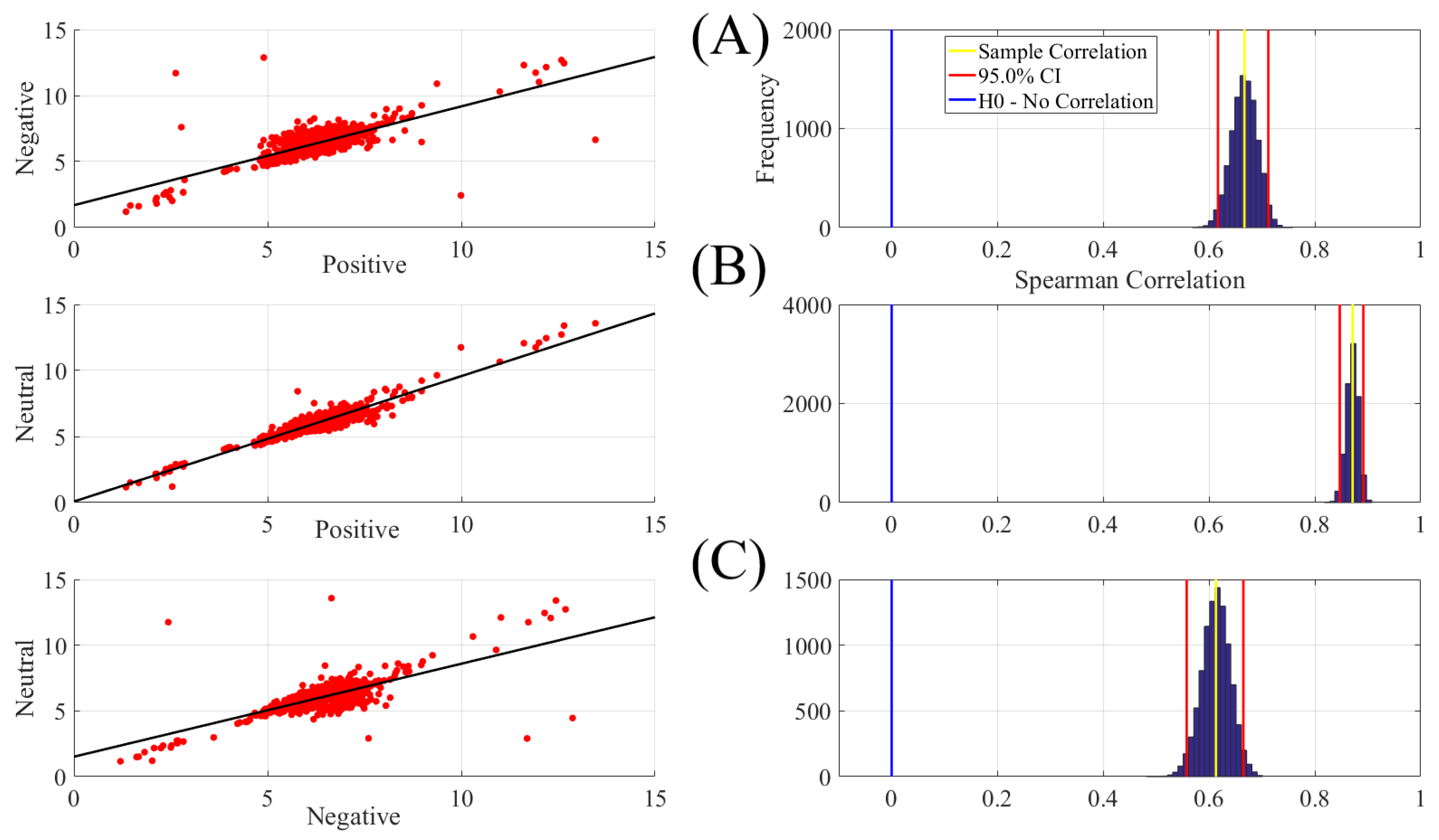
| Conditions | r | p (two-tailed) | CI |
|---|---|---|---|
| Positive vs. Negative | 0.67 | 0.00001 | [0.62 0.71] |
| Positive vs. Neutral | 0.87 | 0.00001 | [0.85 0.89] |
| Negative vs. Neutral | 0.61 | 0.00001 | [0.56 0.66] |
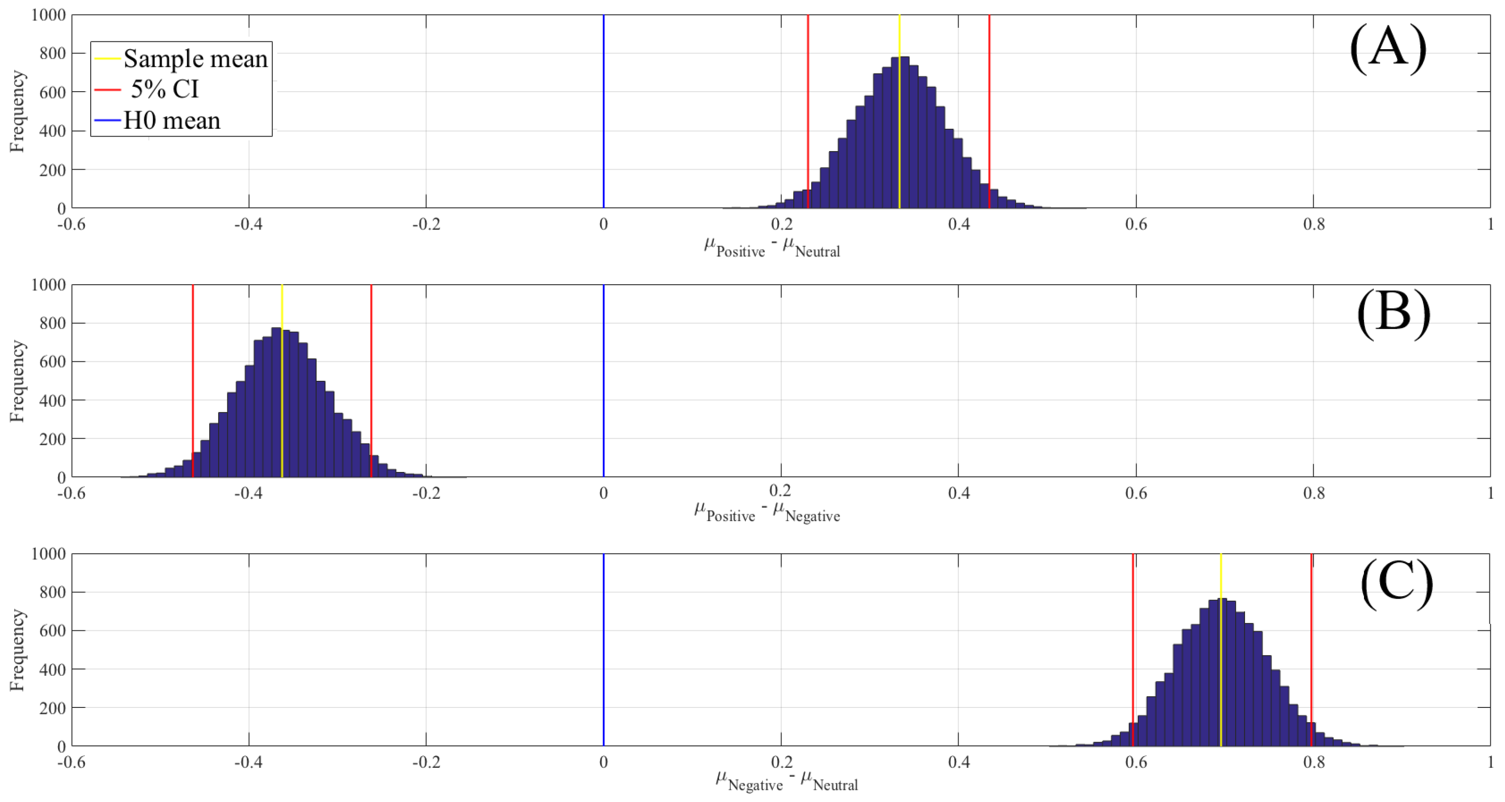
| Conditions | M | SD | 95.0% CI |
|---|---|---|---|
| Positive versus Neutral | 0.33 | 0.05 | [0.23 0.43] |
| Positive versus Negative | 0.05 | [ ] | |
| Negative versus Neutral | 0.70 | 0.05 | [0.60 0.80] |
| Setting | Precision | Recall | F1-Score |
|---|---|---|---|
| Whole-Brain | 0.86 | 0.71 | 0.77 |
| Selected Channels | 0.57 | 0.62 | 0.59 |
© 2019 by the authors. Licensee MDPI, Basel, Switzerland. This article is an open access article distributed under the terms and conditions of the Creative Commons Attribution (CC BY) license (http://creativecommons.org/licenses/by/4.0/).
Share and Cite
Keshmiri, S.; Shiomi, M.; Ishiguro, H. Entropy of the Multi-Channel EEG Recordings Identifies the Distributed Signatures of Negative, Neutral and Positive Affect in Whole-Brain Variability. Entropy 2019, 21, 1228. https://doi.org/10.3390/e21121228
Keshmiri S, Shiomi M, Ishiguro H. Entropy of the Multi-Channel EEG Recordings Identifies the Distributed Signatures of Negative, Neutral and Positive Affect in Whole-Brain Variability. Entropy. 2019; 21(12):1228. https://doi.org/10.3390/e21121228
Chicago/Turabian StyleKeshmiri, Soheil, Masahiro Shiomi, and Hiroshi Ishiguro. 2019. "Entropy of the Multi-Channel EEG Recordings Identifies the Distributed Signatures of Negative, Neutral and Positive Affect in Whole-Brain Variability" Entropy 21, no. 12: 1228. https://doi.org/10.3390/e21121228