Entropy Generation Rate Minimization for Methanol Synthesis via a CO₂ Hydrogenation Reactor

Abstract

The methanol synthesis via CO₂ hydrogenation (MSCH) reaction is a useful CO₂ utilization strategy, and this synthesis path has also been widely applied commercially for many years. In this work the performance of a MSCH reactor with the minimum entropy generation rate (EGR) as the objective function is optimized by using finite time thermodynamic and optimal control theory. The exterior wall temperature (EWR) is taken as the control variable, and the fixed methanol yield and conservation equations are taken as the constraints in the optimization problem. Compared with the reference reactor with a constant EWR, the total EGR of the optimal reactor decreases by 20.5%, and the EGR caused by the heat transfer decreases by 68.8%. In the optimal reactor, the total EGRs mainly distribute in the first 30% reactor length, and the EGRs caused by the chemical reaction accounts for more than 84% of the total EGRs. The selectivity of CH₃OH can be enhanced by increasing the inlet molar flow rate of CO, and the CO₂ conversion rate can be enhanced by removing H₂O from the reaction system. The results obtained herein are in favor of optimal designs of practical tubular MSCH reactors.

1. Introduction

Over the past century, a huge amount of CO₂ produced through burning fossil fuels has been released into the atmosphere, which has led to global warming. Nowadays, much effort is being put into carbon emission reduction. There are mainly three ways to reduce carbon emissions: (1) Utilizing clean energy sources, such as the solar, wind, nuclear, and tidal energy; (2) utilizing carbon sequestration and storage technology; (3) collecting and recycling CO₂ through chemical reactions. The methanol synthesis via CO₂ hydrogenation (MSCH) reaction is in fact an effective scheme for alleviating the greenhouse effect. What is more, methanol is a primary liquid petrochemical, and is widely used in the chemical and energy fields in applications such as hydrogen storage, dimethyl ether and hydrocarbon production, etc. [1,2,3,4].

However, the methanol synthesis via CO₂ hydrogenation reaction still has some problems to be solved, e.g., high energy-consumption, low conversion rate and poor selectivity [5]. So far the studies for MSCH mainly include: (1) developing new catalysts and establishing the corresponding kinetic models [6,7,8]; (2) improving the MSCH reaction process by modeling and simulation [9,10,11,12]; (3) studying the thermodynamic performance of the MSCH reaction based on classical thermodynamic theory [5,13,14].

Thermodynamic equilibrium and reversibility are the main assumptions in classical thermodynamic analysis. The plug flow reactor studied herein involves three irreversible phenomena: the chemical reaction, viscosity flow, and heat transfer, which result in entropy generation [15]. Therefore, the MSCH reactor should been analyzed and optimized based on finite time thermodynamic (FTT) theory [16,17,18,19,20,21,22,23,24,25,26,27,28,29], which has been utilized to optimize irreversible processes and cycles considering the effect of the finite time or size. In the engineering field it is also known as entropy generation minimization [30,31,32,33,34].

Many scholars have generally preferred to make the yield of the target production as the optimization objective function in their performance studies on industrial reactors. In 1986, Månsson and Andresen [35] firstly utilized FTT theory to study the performance of a catalyzed ammonia synthesis reactor and obtained the optimal temperature profile of reaction mixtures corresponding to the objective function of the maximum ammonia yield. Jahanmiri and Eslamloueyan [36] studied the performance of a methanol synthesis reactor and obtained the optimal temperature profile of the reaction mixture corresponding to the objective function of the maximum methanol yield. Farsi and Jahanmiri [37,38,39,40] completed a series of works on the performance of the methanol synthesis membrane reactor for the sake of improving the methanol yield. Wang et al. [41] studied the performance of a sulphuric acid decomposition reactor with the maximum SO₂ yield as the objective function and obtained the optimal exterior wall temperature (EWT) and pressure of reaction mixture (PRM) profiles.

According to Gouy-Stodola theory, the amount of lost work is defined as the product of ambient temperature and the entropy generation of process, so the irreversibility of the process will be reduced by minimizing the entropy generation of the irreversible process [31,32,33,42]. Kjelstrup et al. [43] utilized the MSCH kinetic model established by Bussche and Froment [44] to study the MSCH reactor and obtained the optimal temperature profile of reaction mixture corresponding to the objective function of minimum total entropy generation rate (EGR) caused by the MSCH reaction. Johannessen and Kjelstrup [45] studied the performance of SO₂ oxidation reactor with the EGR minimization as the optimization objective and obtained the optimal EWT profile and reactor length. Nummedal et al. [46] studied the SMR reactor with the EGR minimization as the optimization objective and obtained the optimal EWT profile. Ao et al. [47] and Chen [48] et al. also studied the performances of SMR reactors with the heat transfer laws of linear phenomenological [47] and Dulong-Petit [48], respectively, and obtained the optimal EWT profiles. van der Ham et al. [42] optimized the performance of a sulfuric acid decomposition reactor and obtained two pathways to reduce the EGR in the reactor. Kingston and Razzitte [49,50] studied the EGR of two ideal reactors, the dimethyl ether synthesis reactor with the EGR minimization as the optimization objective and obtained the optimal inlet composition of the reactor. On the basis of these achievements, they also investigated the thermally coupled reactor. Chen et al. [51] established a tubular flow reactor model for the process of CO₂ hydrogenation to light olefins and obtained the optimal design parameters with the minimum specific EGR as the objective function. Chen et al. [52] established a hollow fiber membrane contactor model for extracting CO₂ from seawater and obtained the analytical formulae of the CO₂ extraction rate and the EGR of the process. Zhang et al. [53] established a reverse water-gas shift reaction (RWGS) reactor model based on the experimental data and obtained the optimal configuration for the minimum total EGR of the reactor.

The previous works on the minimum EGR of the industrial reactors indicate that the total EGR of reactor can be reduced by adjusting the reactor length, improving the transport properties, and changing the operation condition. Changing the operation condition is considered as the only approach to reduce the total EGR in this paper, since the EGR caused by the viscous flow is insignificant, and the transport properties depend on the material and catalyst et al. [15]. Kjelstrup et al. [43] optimized the temperature profile corresponding to the minimum total EGR caused by the MSCH reaction. This paper will use FTT theory to optimize the performance of MSCH reactor with the total EGR minimization as the optimization objective and seek the optimal EWT profile and the optimal boundary conditions.

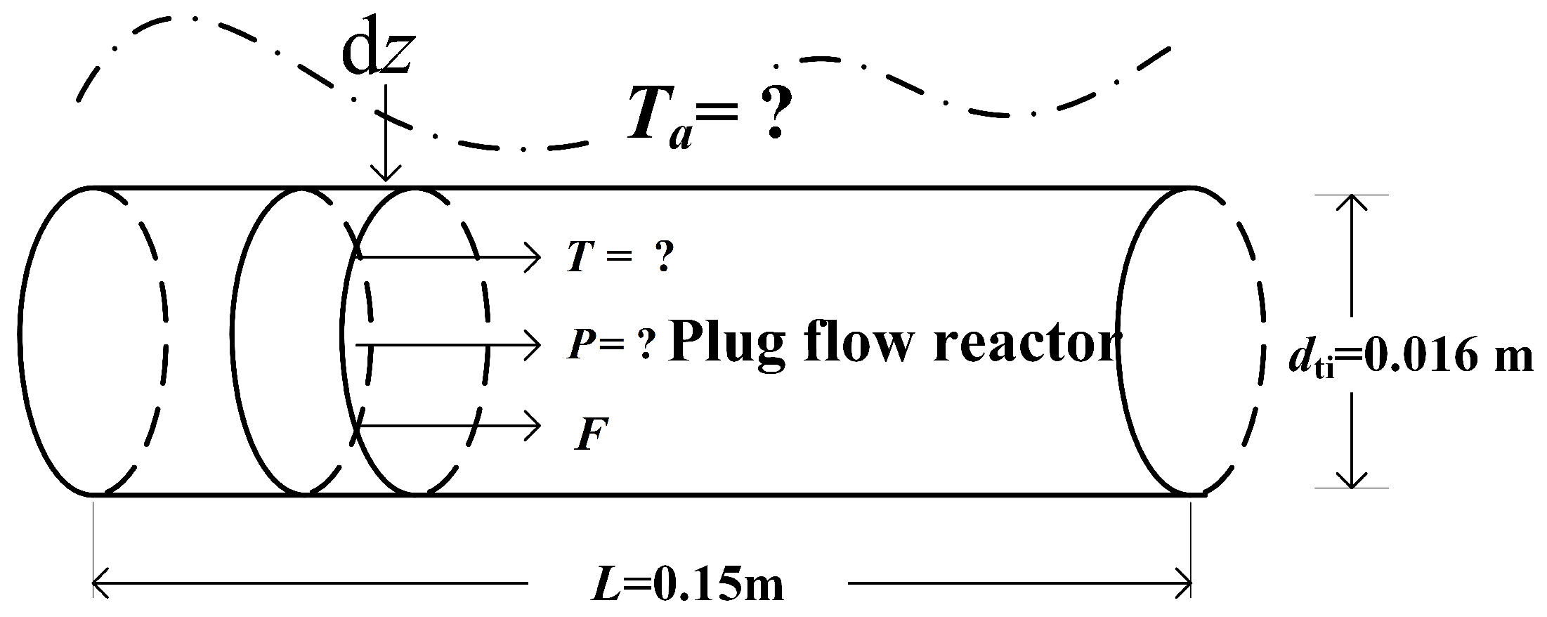
2. Reactor Model and System Description

2.1. Reactor Model

Two routes of methanol synthesis can be found in public literature, i.e., (1) CO₂ shifts to CO through RWGS, and then CO convert into CH₃OH; (2) CO₂ convert into CH₃OH through an intermediate HCOO [3]. Undergo the experimental research of many years, Skrzypel et al. [54] and Vanden Bussche and Froment [55] confirmed that CO₂ is the main source of methanol synthesis, and CO and CO₂ can mutual converts through the RWGS reaction [2,9]. Two reactions occurring in the reactor are as follows [9,36,44]:

$${\mathrm{CO}}_2{+3\mathrm{H}}_2\stackrel{}{\rightleftharpoons }{\mathrm{CH}}_3{\mathrm{OH}+\mathrm{H}}_2\mathrm{O}\hspace{1em}\hspace{1em}\hspace{1em}\hspace{1em}{\mathsf{\Delta }}_r{H}_1<0$$

(1)

$${\mathrm{CO}}_2{+\mathrm{H}}_2\stackrel{}{\rightleftharpoons }\mathrm{CO}+{\mathrm{H}}_2\mathrm{O}\hspace{1em}\hspace{1em}\hspace{1em}\hspace{1em}\hspace{1em}\hspace{1em}{\mathsf{\Delta }}_r{H}_2>0$$

(2)

where ${\mathsf{\Delta }}_r{H}_i$ is the enthalpy of reaction $i$.

In the chemical industrial production, two reactions generally reacts in a suit of catalyst-filled tubes, which are placed inside a tubular heat exchanger. In order to simplify the model, this paper will study one such tube, and establish a one-dimensional pseudo-homogeneous plug flow reactor model as shown in Figure 1 [15,35,41,42,43,44,45,46,47,48,49,50,51,52,53].

According to the judgmental criterion of the assumption on the plug flow, one reactor can be taken as a plug flow reactor, in the case of $L/d_{\mathrm{ti}}$ (L and d_ti are, respectively, the reactor length and diameter) exceeds 150 [56]. Herein, $L/d_{\mathrm{ti}}$ is equal to 300, therefore, the MSCH reactor can be taken as a plug flow reactor. The mathematical model of diffusion listed in Appendix A, Appendix B, and Appendix C are consistent with recent treatments of reaction-diffusion descriptions by Niven [57] and England [58] and a recent temperature-dependent description by Ritchie [59]. The effect of the diffusion within the catalyst pellet on the chemical reaction rate can be ignored, when the effectiveness factor of chemical reaction is close to 1. In this paper, the diffusion within the catalyst pellet can be ignored, and the MSCH reactor can be taken as a pseudo-homogeneous reactor through the verification. The detailed discussion is shown in Appendix A and Appendix B. The MSCH reactor herein can be studied with one-dimensional model, since the size of MSCH reactor is not large, and radial gradient of temperature and mass can be ignored. In summary, the MSCH reactor model herein includes following assumptions: (1) the reaction mixture is not back-mixed in the axial, and mixes uniformly in the radial; (2) the radial temperature and concentration gradients are neglected.

In the MSCH reactor, both the reactants and products are taken as the ideal gas. The reactor geometry parameters, the ICI 51-2 Cu/ZnO/Al₂O₃ catalyst geometry parameters, the physical parameters of mixture gas and the inlet conditions derived from the reference reactor in References [44,45] are listed in

Table 1. Design parameters of the reference reactor [43].

Parameter	Sign	Value
Inlet temperature of reaction mixture	$T_{\mathrm{in}}$	493.2 K
Overall heat transfer coefficient	$U$	$60 \mathrm{W}/(\mathrm{K}·{\mathrm{m}}^2)$
Inlet total pressure	$P_{\mathrm{in}}$	$8.5\times {10}^6 \mathrm{Pa}$
Catalyst density	${\rho }_{\mathrm{c}}$	$1775\hspace{0.17em}{\mathrm{kg}/\mathrm{m}}^3$
Catalyst void fraction	${\epsilon }_{\mathrm{p}}$	0.5
Catalyst pellet diameter	$d_{\mathrm{p}}$	$5\times {10}^{-4}\hspace{0.17em}\mathrm{m}$
Total catalyst weight	$W_{\mathrm{c},\mathrm{Tot}}$	0.0267 kg
Reactor length	$L$	0.15 m
Reactor diameter	$d_{\mathrm{ti}}$	0.016 m
Inlet total mole flow rate	$F_{\mathrm{T},\mathrm{in}}$	0.0033 mol/s
Inlet mole fraction of CO2	$x_{{\mathrm{CO}}_2,\hspace{0.17em}\mathrm{in}}$	0.03
Inlet mole fraction of H2	$x_{{\mathrm{H}}_2,\mathrm{in}}$	0.82
Inlet mole fraction of CO	$x_{\mathrm{CO},\mathrm{in}}$	0.04
Inlet mole fraction of H2O	$x_{{\mathrm{H}}_2\mathrm{O},\mathrm{in}}$	0.005
Inlet mole fraction of CH3OH	$x_{{\mathrm{CH}}_3\mathrm{OH},\hspace{0.17em}\mathrm{in}}$	0.005
Inlet mole fraction of N2	$x_{{\mathrm{N}}_2,\hspace{0.17em}\mathrm{in}}$	0.10

. The overall heat transfer profile of the reference reactor along the dimensionless axial can be obtained based on the empirical formula proposed by Dixonge [60,61], and the calculation results indicate that the overall heat transfer coefficient is approximately equal to 60 $\mathrm{W}/\left(\mathrm{K}·{\mathrm{m}}^2\right)$.

2.2. Reaction Kinetic Model

The MSCH reaction processes can be classified as the high-pressure process, 25–30 MPa, the medium-pressure process, 10–25 MPa, and the low-pressure process, 5–10 MPa [36]. Among them, there are more researches on low-pressure process, since the low-pressure of methanol synthesis process is applied widely in chemical industries [1,3,62].

In this paper, the kinetic model established by Vanden Bussche and Froment [44] is selected and utilized, since this kinetic model is based on the ICI 51-2 Cu/ZnO/Al₂O₃ catalyst, which is applied widely in chemical industries, such as the LURGI type methanol synthesis reactor [9]. Another reason is that the kinetic model proposed by Reference [44] has been checked by experiments of lab-scale [44,55] and commercial-scale [9], what is more, the kinetic model has a wider application range. The temperature varies between 180 and 280 °C, the pressures varies between 15 and 51 bar in the experiment of Vanden Bussche and Froment [44]. The pressure from industrial data of LURGI type methanol synthesis reactor is 66.7 bar [9].

According to the kinetic model proposed by Reference [44], the reaction rates of the MSCH and RWGS reactions are:

$$r_1={\kappa }_1{P}_{{\mathrm{CO}}_2}{P}_{{\mathrm{H}}_2}[1-(1/K_1^{\ast })(P_{{\mathrm{H}}_2\mathrm{O}}{P}_{{\mathrm{CH}}_3\mathrm{OH}}/P_{{\mathrm{H}}_2}^3{P}_{{\mathrm{CO}}_2})]{\beta }^3$$

(3)

$$r_2={\kappa }_2{P}_{{\mathrm{CO}}_2}[1-K_2^{\ast }(P_{{\mathrm{H}}_2\mathrm{O}}{P}_{\mathrm{CO}}/P_{{\mathrm{CO}}_2}{P}_{{\mathrm{H}}_2})]\beta$$

(4)

$$\beta =1/[1+{\kappa }_3(P_{{\mathrm{H}}_2\mathrm{O}}/P_{{\mathrm{H}}_2})+{\kappa }_4\sqrt{P_{{\mathrm{H}}_2}}+{\kappa }_5{P}_{{\mathrm{H}}_2\mathrm{O}}]$$

(5)

$${\log }_{10}(K_1^{\ast })=\frac{3066}{T}-10.592$$

(6)

$${\log }_{10}(K_2^{\ast })=\frac{-2073}{T}+2.029$$

(7)

where $r_i$ is the reaction rate of reaction $i$, $P_{\mathrm{k}}=(P{F}_{\mathrm{k}})/F_{\mathrm{T}}$ is the partial pressure of component $\mathrm{k}$, $P$ and $T$ are the pressure and temperature of reaction mixture (TRM), respectively, $F_{\mathrm{k}}$ and $F_{\mathrm{T}}$ are the mole flow rate of component k and reaction mixture in the axial position $z$, respectively, $K_1^{\ast }$ and $K_2^{\ast }$ are thermodynamic equilibrium constants of Reactions (1) and (2) [63], respectively, and ${\kappa }_j$ is parameter group $j$ related to the adsorption, equilibrium, and rate constants of elementary reactions. These parameter groups can be calculated as follows [44]:

$${\kappa }_j=A(j)\exp [B(j)/R_{g}T]$$

(8)

where $R_{\mathrm{g}}=8.314 \mathrm{J}/\left(\mathrm{mole}·\mathrm{K}\right)$ is the universal gas constant, $A(i)$ is the frequency factor, $B(i)$ represents either $E$ or $-\mathsf{\Delta }H$, and these factors are listed in

Table 2. Kinetic model parameters [44] *.

${\mathit{\kappa }}_{\mathit{j}}$	$\mathit{A}(\mathit{j}),\mathit{B}(\mathit{j})$	Value	${\mathit{\kappa }}_{\mathit{j}}$	$\mathit{A}(\mathit{j}),\mathit{B}(\mathit{j})$	Value
$k_1=k_{5\mathrm{a}}^{\prime }{K}_2^{\prime }{K}_3{K}_4{K}_{{\mathrm{H}}_2}$	A	1.07	$k_2=k_1^{\prime }$	A	$1.22\times {10}^{10}$
	B	36,696		B	−94,765
$k_3=K_{{\mathrm{H}}_2\mathrm{O}}/K_8{K}_9{K}_{{\mathrm{H}}_2}$	A	3453.38	$k_4=\sqrt{K_{{\mathrm{H}}_2}}$	A	0.499
	B	-		B	17,197
$k_5=K_{{\mathrm{H}}_2\mathrm{O}}$	A	$6.62\times {10}^{-11}$	-	-	-
	B	124,119	-	-	-

* $k_{5\mathrm{a}}^{\prime }$ and $k_1^{\prime }$ are, respectively, the rate constants of the rate-determining steps for the MSCH and RWGS reactions, $K_{{\mathrm{H}}_2}$ and $K_{{\mathrm{H}}_2\mathrm{O}}$ are, respectively, the adsorption constants of H₂ and H₂O, $K_{\mathrm{m}}$s (m = 2, 3, 4, 8, 9) are the equilibrium constants of all elementary reactions except for some ignored.

[44].

2.3. Conservation Equation

The heat transfer between the reaction mixture and the exterior wall heat reservoir obeys the Newton heat transfer law, i.e., $q\propto \left(\mathsf{\Delta }T\right)$, and the heat flux passed through the tube wall is

$$J_q=U(T_{\mathrm{a}}-T)$$

(9)

where $U$ is the overall heat transfer coefficient, and $T_{\mathrm{a}}$ is the EWT.

The energy conservation equation is:

$$\frac{\mathrm{d}T}{\mathrm{d}z}=\frac{\pi d_{\mathrm{ti}}{J}_q-{\rho }_{\mathrm{c}}{A}_{\mathrm{c}}\left(1-{\epsilon }_{\mathrm{c}}\right){\displaystyle {\sum }_i{r}_i{\mathsf{\Delta }}_r{H}_{T,i}}}{{\displaystyle {\sum }_k{F}_k{C}_{p,k}}}$$

(10)

where ${\epsilon }_{\mathrm{c}}$ is the void fraction of the catalyst bed, ${\rho }_{\mathrm{c}}$ is the catalyst density, $C_{p,k}$ is the mole heat capacity at constant pressure of the component k, and ${\mathsf{\Delta }}_r{H}_{T,i}$ is the standard mole enthalpy of reaction $i$. These parameters can be obtained as follows [64]:

$$C_{p,k}=A_k+B_{k}T+C_k{T}^2+D_k{T}^3+E_k{T}^4$$

(11)

$${\mathsf{\Delta }}_r{H}_{T,i}={\displaystyle {\sum }_k\left({\upsilon }_{k,i}{\mathsf{\Delta }}_f{H}_{T, k}+I_i\right)}$$

(12)

$${\mathsf{\Delta }}_f{H}_{T, k}=A_{k}T+\left({\upsilon }_{k,i}{B}_k{T}^2\right)/2+\left({\upsilon }_{k,i}{C}_k{T}^3\right)/3+\left({\upsilon }_{k,i}{D}_k{T}^4\right)/4+\left({\upsilon }_{k,i}{E}_k{T}^5\right)/5$$

(13)

$$I_i={\displaystyle {\sum }_k{\upsilon }_{k,i}\left({\mathsf{\Delta }}_f{H}_{298.15\mathrm{K}, k}^0-{\mathsf{\Delta }}_f{H}_{298.15\mathrm{K}, k}\right)}$$

(14)

where ${\upsilon }_{k,i}$ is the stoichiometric number of component $k$ in reaction $i$, $I_i$ is the integration constant of reaction $i$ that can be obtained based on the standard mole enthalpy ${\mathsf{\Delta }}_f{H}_{298.15\mathrm{K}, k}^0$ and the coefficients $A$, $B$, $C$, $D$, $E$, ${\mathsf{\Delta }}_f{H}_{298.15\mathrm{K}}^0$ and $M_k$ are listed in

Table 3. Thermodynamic parameters [66].

	$\begin{array}{l}\mathbf{k}=1\\ ({\mathbf{CO}}_2)\end{array}$	$\begin{array}{l}\mathbf{k}=2\\ ({\mathbf{H}}_2)\end{array}$	$\begin{array}{l}\mathbf{k}=3\\ (\mathbf{CO})\end{array}$	$\begin{array}{l}\mathbf{k}=4\\ ({\mathbf{CH}}_3\mathbf{OH})\end{array}$	$\begin{array}{l}\mathbf{k}=5\\ {(\mathbf{H}}_2\mathbf{O})\end{array}$	$\begin{array}{l}\mathbf{k}=6\\ ({\mathbf{N}}_2)\end{array}$
$A_{\mathrm{k}}$	27.4370	25.3990	29.5560	40.0460	33.9330	29.3420
$B_{\mathrm{k}}(\times {10}^{-3})$	42.3150	20.1780	−6.5807	−3.8287	−8.4186	−3.5395
$C_{\mathrm{k}}(\times {10}^{-5})$	−1.9555	−3.8549	2.0130	24.5290	2.9906	1.0076
$D_{\mathrm{k}}(\times {10}^{-8})$	3.9968	31.8800	−12.2270	−216.7900	−17.8250	−4.3116
$E_{\mathrm{k}}(\times {10}^{-11})$	−2.9872	−87.5850	22.6170	599.0900	36.9340	2.5935
${\mathsf{\Delta }}_f{H}_{298.15\mathrm{K}}$$(\mathrm{kJ}/\mathrm{mol})$	−393.50	0	−110.50	−201.17	−241.80	191.6
$M_{\mathrm{k}} \left(\mathrm{g}/\mathrm{mol}\right)$	44.01	2.016	28.01	32.042	18.015	28.013

[65].

The momentum equation utilized to describe the pressure drop along the reactor axial is generally described by the Ergun equation, in the case of $R{e}_{\mathrm{p}}/(1-{\epsilon }_{\mathrm{c}})<500$ [66]. The Reynolds numbers $R{e}_{\mathrm{p}}$ is:

$$R{e}_{\mathrm{p}}=G{d}_{\mathrm{p}}/{\mu }_{\mathrm{mix}}$$

(15)

where $G$ is the superficial mass flow rate, $G={\displaystyle {\sum }_k\left(F_k{M}_k\right)}/A_{\mathrm{c}}$, $M_k$ is the mole mass of component $k$, ${\mu }_{\mathrm{mix}}$ is the viscosity of reaction mixture (see Appendix C), and $d_{\mathrm{p}}$ is the catalyst particle diameter.

$R{e}_{\mathrm{p}}/(1-{\epsilon }_{\mathrm{c}})$ is less than 0.005 in the case discussed in this paper, therefore, the momentum equation can be described by the Ergun equation as follows:

$$\frac{\mathrm{d}P}{\mathrm{dz}}=-\left[\frac{150{\mu }_{\mathrm{mix}}(1-{\epsilon }_{\mathrm{c}})}{d_{\mathrm{p}}^{}}+1.75G\right]\frac{c_{\mathrm{g}}}{d_{\mathrm{p}}}\frac{\left(1-{\epsilon }_{\mathrm{c}}\right)}{{\epsilon }^3}$$

(16)

where $c_{\mathrm{g}}=F_{\mathrm{T}}{R}_{\mathrm{g}}T/(P{A}_{\mathrm{c}})$ is the superficial velocity of mixture gas.

The mole balance equations are described by the yields of CH₃OH and CO (${\xi }_1$ and ${\xi }_2$), which are both defined with the inlet mole flow rate of CO₂ [15]:

$$\frac{\mathrm{d}{\xi }_1}{\mathrm{dz}}={\rho }_{\mathrm{c}}{A}_{\mathrm{c}}\left(1-{\epsilon }_{\mathrm{c}}\right)\frac{r_1}{F_{{\mathrm{CO}}_2,\mathrm{in}}}$$

(17)

$$\frac{\mathrm{d}{\xi }_2}{\mathrm{dz}}={\rho }_{\mathrm{c}}{A}_{\mathrm{c}}\left(1-{\epsilon }_{\mathrm{c}}\right)\frac{r_2}{F_{{\mathrm{CO}}_2,\mathrm{in}}}$$

(18)

where subscript ‘in’ denotes the inlet state of variables, and the mole flow rate of component $k$ and the total mole flow rate are defined as follows:

$$F_k=F_{k,\mathrm{in}}+F_{{\mathrm{CO}}_2,\mathrm{in}}{\displaystyle {\sum }_i{\upsilon }_{i,k}{\xi }_i}$$

(19)

$$F_T=F_{T,\mathrm{in}}-2F_{{\mathrm{CO}}_2,\mathrm{in}}{\xi }_1$$

(20)

2.4. Entropy Generation Rate of the MSCH Reactor

Non-equilibrium thermodynamics indicates that the irreversible process always generates EGR, which is described as the product sum of the conjugate fluxes and forces [67,68,69]. In a plug flow reactor, the EGR is mainly produced by the chemical reactions, heat transfer and viscous flow [15,67,68,69].

In term of the EGR due to chemical reactions, the driving forces are:

$$-\frac{{\mathsf{\Delta }}_r{G}_1}{T}=-R_{\mathrm{g}}\ln \frac{P_{{\mathrm{CH}}_3\mathrm{OH}}{P}_{{\mathrm{H}}_2\mathrm{O}}^{}}{P_{{\mathrm{CO}}_2}{P}_{{\mathrm{H}}_2}^3{K}_1^{\ast }}$$

(21)

$$-\frac{{\mathsf{\Delta }}_r{G}_2}{T}=-R_{\mathrm{g}}\ln \frac{P_{\mathrm{CO}}{P}_{{\mathrm{H}}_2\mathrm{O}}}{P_{{\mathrm{CO}}_2}{P}_{{\mathrm{H}}_2}{K}_2^{\ast }}$$

(22)

where ${\mathsf{\Delta }}_r{G}_i$ is the Gibbs free energy of reaction $i$.

In term of the EGR due to heat transfer, the driving force is:

$$\mathsf{\Delta }(1/T)=\frac{1}{T}-\frac{1}{T_{\mathrm{a}}}$$

(23)

In term of the EGR due to viscous flow, the driving force is:

$$-\frac{\mathrm{d}P}{T\mathrm{dz}}$$

(24)

The local EGR is:

$${\sigma }_{\mathrm{TOT}}=\pi {\mathrm{d}}_{ti}{J}_q\left(\frac{1}{T}-\frac{1}{T_a}\right)+{\rho }_{\mathrm{c}}{A}_{\mathrm{c}}\left(1-\epsilon \right){\displaystyle {\sum }_i{r}_i}\left(\frac{-{\mathsf{\Delta }}_r{G}_i}{T}\right)-A_{\mathrm{c}}{c}_{\mathrm{g}}\frac{1}{T}\frac{\mathrm{d}P}{\mathrm{dz}}$$

(25)

where the three terms on right side are the local EGR due to heat transfer, ${\sigma }_{\mathrm{H}}$, MSCH reaction, ${\sigma }_{\mathrm{MS}}$, RWGS reaction, ${\sigma }_{\mathrm{RW}}$, and viscous flow, ${\sigma }_{\mathrm{F}}$, respectively, and the total EGR, ${\left(\mathrm{d}S/\mathrm{d}t\right)}_{\mathrm{TOT}}$ obtained by the integral of the local EGR along the reactor axial is as follows:

$${\left(\frac{\mathrm{d}S}{\mathrm{d}t}\right)}_{\mathrm{TOT}}={\displaystyle {\int }_0^L{\sigma }_{\mathrm{TOT}}\left(z\right)}\mathrm{dz}={\sum }_{\mathrm{H}}+{\sum }_{\mathrm{MS}}+{\sum }_{\mathrm{RW}}+{\sum }_{\mathrm{F}}$$

(26)

where ${\sum }_{\mathrm{H}}$, ${\sum }_{\mathrm{MS}}$, ${\sum }_{\mathrm{RW}}$ and ${\sum }_{\mathrm{F}}$ are, respectively, the total EGR due to heat transfer, MSCH reaction, RWGS reaction and viscous flow.

The optimization objective is:

$$\mathrm{Min} {\left(\frac{\mathrm{d}S}{\mathrm{d}t}\right)}_{\mathrm{TOT}}=\mathrm{Min}\left[{\displaystyle {\int }_0^{\mathrm{L}}{\sigma }_{\mathrm{TOT}}\left(z\right)\mathrm{d}}\mathrm{z}\right]$$

(27)

Equation (27) takes into account almost all phenomena generating EGR in the MSCH reactor, while Reference [43] only considered the EGR from the MSCH reaction. Therefore, the study for the optimal reactor herein is more comprehensive, and the optimal results can be favorable for the optimal design for the practical MSCH reactor.

3. Mathematical Description of the Optimization Problem

The optimization problem herein is to minimize the total EGR subjected to some constraints. The fixed methanol yield (${\xi }_1=1.3139$, $\mathsf{\Delta }{F}_{{\mathrm{CH}}_3\mathrm{OH}}=1.32\times {10}^{-4}$) and the conservation equations are taken as the constraints. The control variable, i.e., the EWT can be controlled completely. The inlet PRM and the inlet mole flow rate of components in the optimal reactor are same with those in the reference reactor [43]. At the outlet, all variables except for the methanol yield are allowed to change freely. The geometry sizes and the catalyst properties are same with those of the reference reactor in Reference [43]. Optimal control theory is utilized to solve this optimization problem and to find the optimal EWT profile.

3.1. Application of Optimal Control Theory

In the early 1950s, optimal control theory had been applied in the study of the minimum time control problem. However, the original optimal control theory cannot solve an optimization problem that the admissible control belongs to a closed set. In order to solve this problem, Pontryagin created the minimum principle on 1958 [70].

The purpose of this paper is to minimize the total EGR of the MSCH reactor and find the optimal EWT profile by using optimal control theory. Therefore, the EWT is taken as the control variable, the total EGR is taken as the performance objective, and the TRM ($T$), PRM ($P$), methanol yield (${\xi }_1$), and carbon monoxide yield (${\xi }_2$) are taken as the state variables controlled by the conservation equations. The inlet and outlet values of state variables and the multiplier functions corresponding to the state variables are taken as the boundary condition [15].

The Hamiltonian can be established as follow [15,42,70]:

$$H={\sigma }_{\mathrm{TOT}}+{\lambda }_T\frac{dT}{dz}+{\lambda }_P\frac{dP}{dz}+{\lambda }_{{\xi }_1}\frac{d{\xi }_1}{dz}+{\lambda }_{{\xi }_2}\frac{d{\xi }_2}{dz}$$

(28)

where ${\lambda }_T$, ${\lambda }_P$, ${\lambda }_{{\xi }_1}$, and ${\lambda }_{{\xi }_2}$ are the multiplier functions of state variables.

According to the minimum principle of Pontryagin [70], the necessary conditions for the EGR minimization, i.e., canonical Equations, are as follows:

$$\partial T/\partial z=\partial H/\partial {\lambda }_T$$

(29)

$$\partial P/\partial z=\partial H/\partial {\lambda }_P$$

(30)

$$\partial {\xi }_1/\partial z=\partial H/\partial {\xi }_1$$

(31)

$$\partial {\xi }_2/\partial z=\partial H/\partial {\xi }_2$$

(32)

$$\partial {\lambda }_T/\partial z=-\partial H/\partial T$$

(33)

$$\partial {\lambda }_P/\partial z=-\partial H/\partial P$$

(34)

$$\partial {\lambda }_{{\xi }_1}/\partial z=-\partial H/\partial {\xi }_1$$

(35)

$$\partial {\lambda }_{{\xi }_2}/\partial z=-\partial H/\partial {\xi }_2$$

(36)

where Equations (29)–(32) are state equations, and Equations (33)–(36) are adjoint Equations.

Hamiltonian also needs to satisfy the extremum condition, i.e., $\partial H/\partial T_{\mathrm{a}}=0$. The relation between the EWT and the TRM can be derived via this extremum condition [15]:

$$T_{\mathrm{a}}=T{(1+\frac{{\lambda }_{T}T}{{\displaystyle {\sum }_k{F}_k{C}_{p,k}}})}^{-1/2}$$

(37)

The boundary conditions of optimal control theory are obtained based on the transversal condition, i.e., $x_{\mathrm{n}}=x_{\mathrm{n},\mathrm{specification}} \mathrm{or} {\lambda }_{\mathrm{n}}=0$. The boundary conditions are listed in

Table 4. Boundary conditions of optimal control problems *.

	$\mathit{T}$	$\mathit{P}$	${\mathit{\xi }}_1$	${\mathit{\xi }}_2$
$x(0)$	-	85 bar	0	0
$\lambda (0)$	0	-	-	-
$x(z)$	-	-	1.323	-
$\lambda (z)$	0	0	-	0

* $x(0)$ and $x(z)$ are, respectively, the inlet and outlet values of state variables, $\lambda (0)$ and $\lambda (z)$ are, respectively, the multiplier functions of the corresponding state variables at the inlet and outlet.

. The property of Hamilton [70] is often used to check the veracity of the optimal results. Hamiltonian herein keeps on a constant along the optimal trajectory, since it does not depend on explicitly the axial reactor length, i.e., Hamiltonian is autonomous.

3.2. Numerical Calculations of Optimization Problem

Solving the optimization problem must has a reasonable initial value. The calculation results of the reference reactor with constant heat reservoir $T_{\mathrm{a}}=523 \mathrm{K}$ [43] solved by the numerical discretization are taken as the initial values of the optimal reactor. Optimization problem herein involves eight differential equations, i.e., (Equations (29)–(36)), 1 algebraic equation, i.e., Equation (37), and eight boundary conditions listed in Table 4. Therefore, the optimal control comes down to solve a two-point boundary value problem involving the differential equation. Optimal solution can be obtained by the ‘bvp4c’ solver in Matlab. The solution accuracy is mainly influenced by the initial multiplier functions, i.e., ${\lambda }_{{\xi }_1}$, ${\lambda }_{{\xi }_2}$, and the number of grid points. In order to improve the solution accuracy, this paper utilizes 5000 grid points. The calculation results show that the solution error does not exceed $6.0\times {10}^{-8}$.

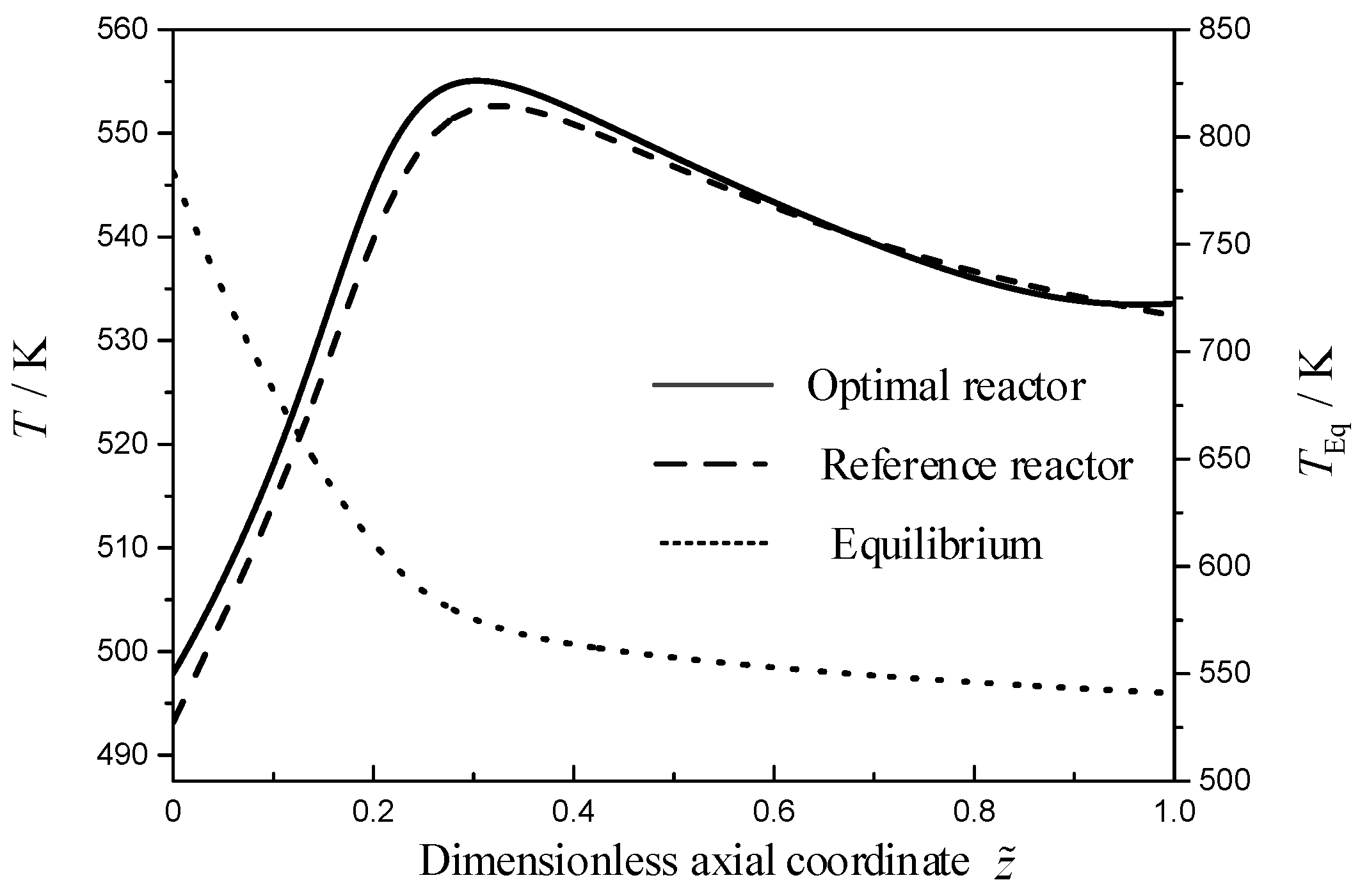
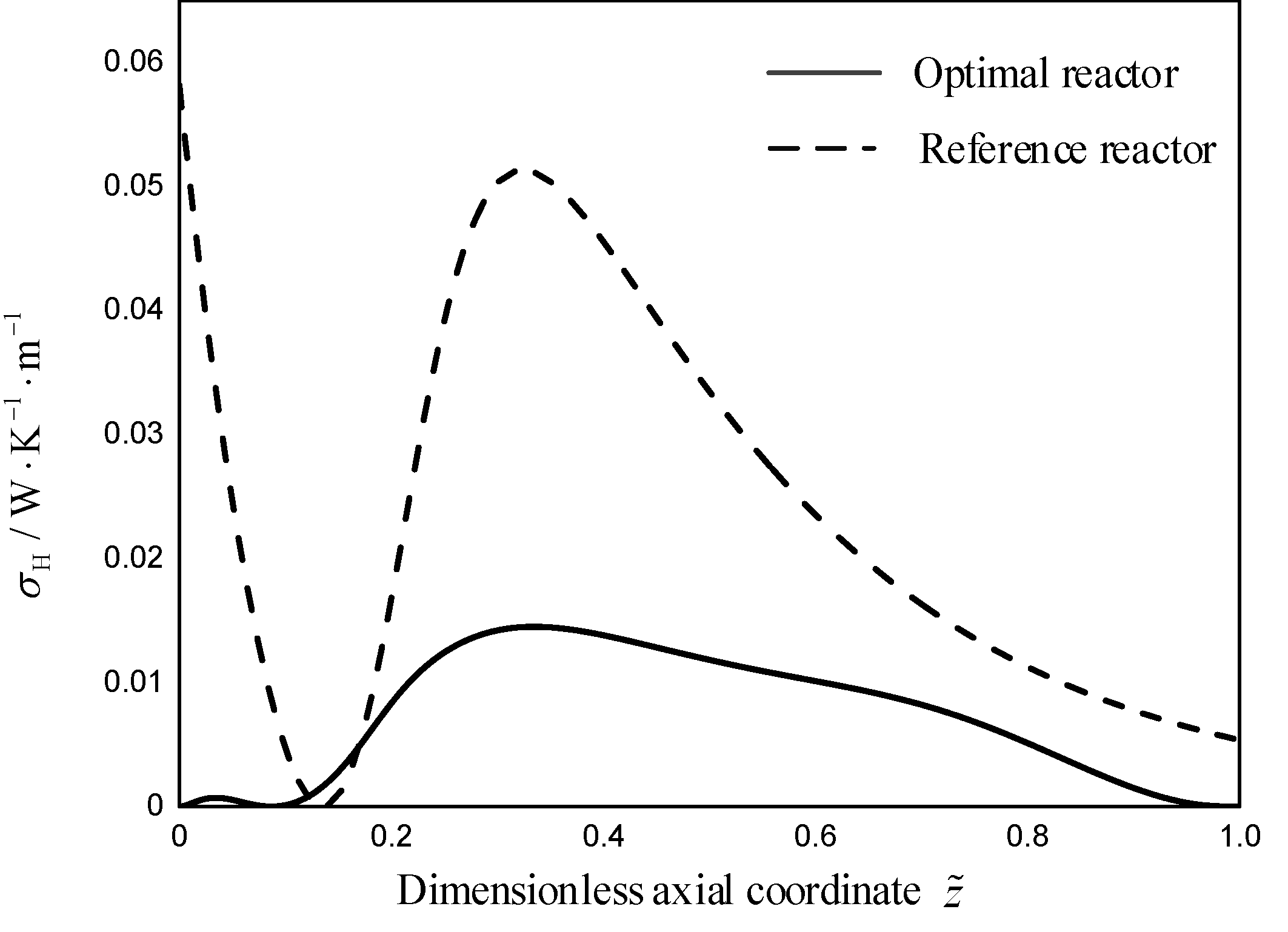
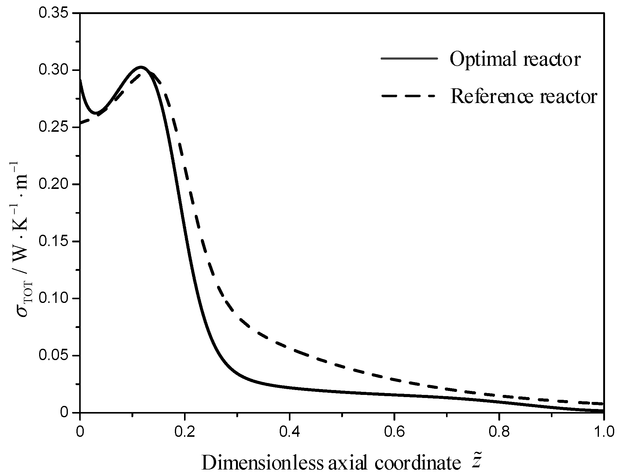
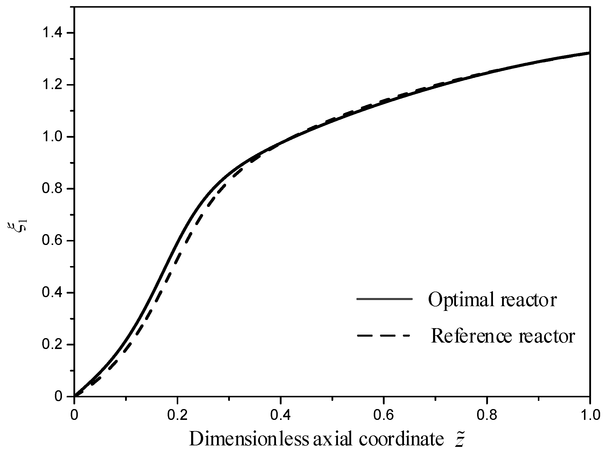
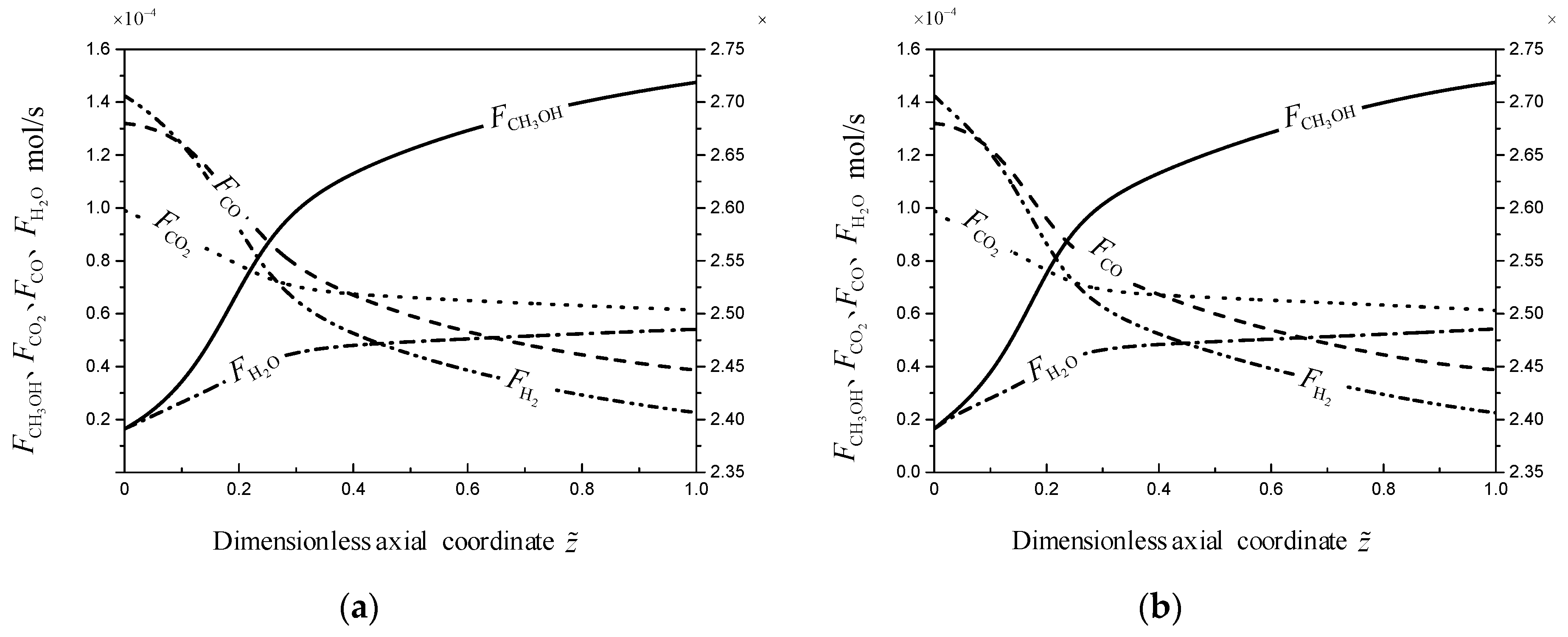
4. Numerical Results and Discussions

The reference reactor with the constant heat reservoir $T_{\mathrm{a}} = 523 \mathrm{K}$ and the optimal reactor with minimum EGR due to the MSCH reaction [43], i.e., the optimal reactor in [43] are both utilized to compare with the optimal reactor herein, i.e., the optimal reactor. In the three reactors, the geometry sizes of reactor, the catalyst properties, and the inlet components are the same with those of the reference reactor in Reference [43].

Table 5. EGR of the three reactors *.

$\mathbf{d}\mathit{S}/\mathbf{d}\mathit{t} \left(\mathbf{W}/\mathbf{K}\right)$	${\mathit{T}}_{\mathbf{a}}=\mathbf{const}$	$\mathbf{d}{\mathit{S}}_{\mathbf{chem}}^1/\mathbf{d}\mathit{t}=\mathbf{min}$ [45]	$\mathbf{d}{\mathit{S}}_{\mathbf{T}}/\mathbf{d}\mathit{t}=\mathbf{min}$
Reaction 1	$1.66\times {10}^{-3}$	$3.80\times {10}^{-4}$	$1.60\times {10}^{-3}$
Reaction 2	$1.05\times {10}^{-4}$	$3.71\times {10}^{-5}$	$9.94\times {10}^{-5}$
Heat transfer	$6.28\times {10}^{-4}$	$4.94\times {10}^{-3}$	$1.96\times {10}^{-4}$
Viscous flow	$1.89\times {10}^{-7}$	-	$1.90\times {10}^{-7}$
Total EGR	$2.39\times {10}^{-3}$	$5.35\times {10}^{-3}$	$1.90\times {10}^{-3}$

* The symbols $T_{\mathrm{a}}=\mathrm{const}$, $\mathrm{d}{S}_{\mathrm{chem}}^1/\mathrm{d}t=\min$, and $\mathrm{d}{S}_{\mathrm{T}}/\mathrm{d}t=\min$ represent the reference reactor and optimal reactor in Reference [45], and the optimal reactor herein, respectively.

lists the total EGRs of the three reactors. Compared with the results of the reference reactor in [43], the total EGR of the optimal reactor decreases by 20.5%, the total EGR due to the heat transfer decreases by 68.8%, the total EGR due to two chemical reactions decreases by 3.3%, and the total EGR due to the viscous flow is almost unchanged. In the reference and optimal reactors, the total EGRs due to the MSCH reaction account for 69% and 84% of the total EGR, respectively. In the optimal reactor of [43], the total EGR due to the MSCH reaction only accounts for 7.1% of the total EGR, however, the total EGR increases by 123.9% compared with that of the reference reactor.

Figure 2 describes the TRM profiles of the reference and optimal reactors, and the equilibrium temperature profile of the MSCH reaction in reference reactor. As shown in Figure 2, the TRM in the reference reactor (dashed line) increases from 493.2 K at the reactor inlet up to a hot spot of 552.6 K, and then it decreases toward a value of 532.4 K. The TRM in the optimal reactor (solid line) increases from 497.9 K at the reactor inlet up to a hot spot of 555.1 K, next it decreases toward a value of 533.4 K, and then it increases toward a value of 533.5 K at the reactor outlet. Except for the range near the reactor outlet, the TRM profiles in the two reactors are almost the same. The above results can be explained according to the theory of the chemical reaction equilibrium, i.e., Le Chatelier’s principle. As shown in Figure 2, the equilibrium temperature of the MSCH reaction (the calculation results based on Equation (22)) decreases steeply from 783.6 K at the reactor inlet up to a turning point of 588 K at the dimensionless axial position $\tilde{z}=0.25$, and then levels off to a more flat decrease until a value of 540.9 K. Near to the inlet of the two reactors, the difference between the TRMs and equilibrium temperature is so large that the chemical driving force is large and the reaction rate is also large. Therefore, a large amount of heat is released by the MSCH reaction, which results into the steep increase of the TRM. With the decrease of the difference between the TRM and equilibrium temperature, the EWTs (as shown in Figure 3) become the dominating contribution to the TRMs. Therefore, the TRMs show a flat decrease under the cooling effect of the EWTs.

Figure 3 describes the EWT profiles of the reference and optimal reactors along the reactor axial. It is noteworthy that the optimal EWT profile (solid line) shown in Figure 3 is a significant result herein. In industrial, this ideal EWT profile can be reached approximately through assigning some heat exchanger providing different constant cooling temperature, e.g., two-stage cooling strategy (dash dot line) in this case can reduce the total EGR 10.78% with respect to the reference reactor. As shown in Figure 3, the EWT in reference reactor (dash line) shows a constant profile along the reactor axial. The EWT in the optimal reactor increases from 497.9 K up to a local maximum of 539.2 K at the dimensionless axial position $\tilde{z}=0.29$, next it decreases to a local minimum of 526.7 K at the dimensionless axial position $\tilde{z}=0.78$, and then it increases to a maximum of 533.6 K at the reactor outlet.

Figure 4 describes that the optimal EWT (solid line) and TRM (dashed line) profiles in the optimal (large frame) and reference reactors (small frame). As shown in large frame of Figure 4, the EWT is almost all less than the TRM. According to the Le Chatelier’s principle, decreasing the TRM is favor of increasing the carbon dioxide conversion and methanol production rates for the endothermic reaction. Therefore, the EWT should be lower than the TRM. It is noteworthy that the EWTs are equal to the TRMs at the inlet and outlet in the optimal reactor. The reason for this phenomenon is that the EWT is equal to the TRM, in the case of the TRM changes freely at the boundary according to optimal control theory.

As shown in Figure 4, the temperature difference in the optimal reactor between the TRM and EWT is almost all less than that in the reference reactor. Therefore, the local EGR due to the heat transfer in the optimal reactor is less than that in the reference reactor (as shown in Figure 5). As shown in Figure 5 and Figure 6, compared with the reference reactor, the local EGR and driving force due to the heat transfer in the optimal reactor distribute more smooth which is in accordance with the equipartition principle of entropy generation and driving force [15,71,72,73,74].

Figure 7 describes the local EGR profiles of the two reactors. As shown in Figure 7, more than 75% of the total EGR distributes in the first 30% length of the two reactors. The local EGR of the optimal reactor (solid line) decreases from 0.2911 $\mathrm{W}/(\mathrm{K}·\mathrm{m})$ up to a local minimum of 0.2623 $\mathrm{W}/(\mathrm{K}·\mathrm{m})$ at the dimensionless axial position $\tilde{z}=0.029$, next it increases toward a value of 0.3025 $\mathrm{W}/(\mathrm{K}·\mathrm{m})$ at the dimensionless axial position $\tilde{z}=0.115$, next it decreases steeply toward a value of 0.028 $\mathrm{W}/(\mathrm{K}·\mathrm{m})$ at the dimensionless axial position $\tilde{z}=0.33$, and then it levels off to a more flat decrease until a value of 0.002 $\mathrm{W}/(\mathrm{K}·\mathrm{m})$ at the reactor outlet. Compared with the local EGR of the reference reactor (dash line), the local EGR of the optimal reactor distribute more even, especially after $\tilde{z}=0.33$. At the first 30% length of the two reactors, the dominating contribution for the local EGR comes from the MSCH reaction, after 30% length, the dominating contribution for the local EGR comes from the heat transfer.

Figure 8 describes the contributions of the heat transfer (dotted line), viscous flow (shot dot line), MSCH reaction (solid line) and RWGS reaction (dashed line) on the local EGR in the two reactors. As shown in Figure 8, the contribution of the MSCH reaction on local EGRs are maximal in the two reactors. After the dimensionless axial position $\tilde{z}=0.35$, the dominating contribution for the local EGR comes from the heat transfer. The local EGR caused by the viscous flow is minimal, since the size of the lab-scale reactor herein is so small that the pressure drop is negligible. However, the local EGR due to viscous flow cannot be ignored in practical methanol synthesis reactor. It is noteworthy that compared with other profiles, the local EGR profiles due to the heat transfer change most dramatically. The reason of this phenomenon is that under the constraints of fixed methanol yield and fixed reactor, the EGR due to heat transfer can be minimized in a larger optimization potential.

Figure 9 describes the methanol yields of the two reactors. As shown in Figure 9, the profiles of the methanol yields of the two reactors are similar, since the outlet methanol yields of the two reactors are fixed. The inlet methanol yield is slightly larger than that of the reference reactor, since the initial MSCH reaction rate in the optimal reactor is slightly larger than that in the reference reactor.

Figure 10 describes mole flow rates of components in the two reactors. The mole flow rate of N₂ is not given, since N₂ doesn’t participate in the MSCH and RWGS reactions. As shown in Figure 10, the mole flow rate of CO decreases over the overall reactor, since the concentration of CO in reaction mixture exceeds the equilibrium concentration of CO under the TRM, which results in that the reaction direction of RWGS is changed. Undoubtedly, the reverse reaction of the RWGS reaction is beneficial for improving the reaction selectivity. The mole flow rate of H₂O increases over the overall reactor. During the reaction process, with the increase of H₂O, the MSCH reaction tends to reach the chemical equilibrium, which goes against the increase of methanol yield.

5. Conclusions

This paper studies the performance of MSCH reactor and obtains the optimal configuration of the EWT using FTT theory. The minimum EGR caused by heat transfer, viscous flow and chemical reaction is taken as the optimization objective, the fixed methanol yield, the fixed inlet pressure, and the fixed inlet components are taken as the constraints, and the completely controllable EWT is taken as the control variable. The mathematical model of the optimization problem is established using optimal control theory. The optimal results indicate that the total EGR decreases by 20.5% and the EGR due to heat transfer decreases by 68.8% compared with that of the reference reactor with a constant EWT profile. The local EGRs of the two reactors mainly distribute in the first 30% reactor length, and the EGRs due to the MSCH reaction account for more than 75%. The local EGR and driving force due to heat transfer in the optimal reactor distribute more evenly, which accords with the principle of equipartition of the entropy generation and driving force. With the increase of CO at reactor inlet, the CH₃OH selectivity will increase. The CO₂ conservation rate can be enhanced by removing H₂O produced in the reaction process. The results obtained herein are in favor of the optimal designs of practical tubular reactors. In order to increase the exergy efficiency of the methanol system, the minimum EGR of the overall system involving the chemical reactor, heat exchanger, compressor, et. al. will be taken as the optimization objective in the future work.

References

1. Lange, J. Methanol synthesis: A short review of technology improvements. Catal. Today 2001, 64, 3–8. [Google Scholar] [CrossRef]
2. Olah, G.A.; Prakash, G.K.; Goeppert, A. Anthropogenic chemical carbon cycle for a sustainable future. J. Am. Chem. Soc. 2011, 133, 12881–12898. [Google Scholar] [CrossRef] [PubMed]
3. Jadhav, S.G.; Vaidya, P.D.; Bhanage, B.M.; Joshi, J.B. Catalytic carbon dioxide hydrogenation to methanol: A review of recent studies. Chem. Eng. Res. Des. 2014, 92, 2557–2567. [Google Scholar] [CrossRef]
4. Morgan, E.R.; Acker, T.L. Practical experience with a mobile methanol synthesis device. J. Sol. Energy Eng. Trans. ASME 2015, 137, 064506. [Google Scholar] [CrossRef]
5. Zhu, H.; Wang, D.F.; Chen, Q.Q.; Shen, G.F.; Tang, Z.Y. Thermodynamic analysis of CO2 hydrogenation to methanol. Nat. Gas Tech. Econ. 2015, 40, 21–25. (In Chinese) [Google Scholar]
6. Huš, M.; Dasireddy, V.D.B.C.; Štefančič, N.S.; Likozar, B. Mechanism, kinetics and thermodynamics of carbon dioxide hydrogenation to methanol on Cu/ZnAl2O4 spinel-type heterogeneous catalysts. Appl. Catal. B Environ. 2017, 207, 267–278. [Google Scholar] [CrossRef]
7. Choi, E.; Song, K.; An, S.; Lee, K.Y.; Youn, M.; Park, K.; Jeong, S.; Kim, H.J. Cu/ZnO/AlOOH catalyst for methanol synthesis through CO2 hydrogenation. Korean J. Chem. Eng. 2018, 35, 73–81. [Google Scholar] [CrossRef]
8. Schneidewind, J.; Adam, R.; Baumann, W.; Jackstell, R.; Beller, M. Low-temperature hydrogenation of carbon dioxide to methanol with a homogeneous cobalt catalyst. Angew. Chem. Int. Edit. 2017, 129, 1916–1919. [Google Scholar] [CrossRef]
9. Chen, L.; Jiang, Q.Z.; Song, Z.Z.; Chen, L. Optimization of inlet temperature of methanol synthesis reactor of LURGI type. Adv. Mater. Res. 2012, 443–444, 671–677. [Google Scholar] [CrossRef]
10. Atsonios, K.; Panopoulos, K.D.; Kakaras, E. Thermocatalytic CO2 hydrogenation for methanol and ethanol production: Process improvements. Int. J. Hydrog. Energy 2016, 41, 792–806. [Google Scholar] [CrossRef]
11. Nimkar, S.C.; Mewada, R.K.; Rosen, M.A. Exergy and exergoeconomic analyses of thermally coupled reactors for methanol synthesis. Int. J. Hydrog. Energy 2017, 42, 28113–28127. [Google Scholar] [CrossRef]
12. Zachopoulos, A.; Heracleous, E. Overcoming the equilibrium barriers of CO2 hydrogenation to methanol via water sorption: A thermodynamic analysis. J. CO2 Util. 2017, 21, 360–367. [Google Scholar] [CrossRef]
13. Fornero, E.L.; Chiavassa, D.L.; Bonivardi, A.L.; Baltanás, M.A. CO2 Capture via catalytic hydrogenation to methanol: Thermodynamic limit vs. ‘kinetic limit’. Catal. Today 2011, 172, 158–165. [Google Scholar] [CrossRef]
14. Gaikwad, R.; Bansode, A.; Urakawa, A. High-pressure advantages in stoichiometric hydrogenation of carbon dioxide to methanol. J. Catal. 2016, 343, 127–132. [Google Scholar] [CrossRef] [Green Version]
15. Johannessen, E.; Kjelstrup, S. A highway in state space for reactors with minimum entropy production. Chem. Eng. Sci. 2005, 60, 3347–3361. [Google Scholar] [CrossRef]
16. Andresen, B.; Berry, R.S.; Ondrechen, M.J.; Salamon, P. Thermodynamics for processes in finite time. Acc. Chem. Res. 1984, 17, 266–271. [Google Scholar] [CrossRef]
17. Chen, L.G.; Wu, C.; Sun, F.R. Finite time thermodynamic optimization or entropy generation minimization of energy system. J. Non-Equilib. Thermodyn. 1999, 24, 327–359. [Google Scholar] [CrossRef]
18. Hoffman, K.H.; Burzler, J.M.; Fischer, A.; Schaller, M.; Schubert, S. Optimal process paths for endoreversible systems. J. Non Equilib. Thermodyn. 2003, 28, 233–268. [Google Scholar] [CrossRef]
19. Chen, L.G. Finite-Time Thermodynamic Analysis of Irreversible Processes and Cycles; Higher Education Press: Beijing, China, 2005. (In Chinese) [Google Scholar]
20. Andresen, B. Current trends in finite-time thermodynamics. Angew. Chem. Int. Edit. 2011, 50, 2690–2704. [Google Scholar] [CrossRef]
21. Kosloff, R. Quantum thermodynamics: A dynamical viewpoit. Entropy 2013, 15, 2100–2128. [Google Scholar] [CrossRef]
22. Ge, Y.L.; Chen, L.G.; Sun, F.R. Progress in finite time thermodynamic studies for internal combustion engine cycles. Entropy 2016, 18, 139. [Google Scholar] [CrossRef]
23. Bi, Y.H.; Chen, L.G. Finite Time Thermodynamic Optimization for Air Heat Pumps; Science Press: Beijing, China, 2017. (In Chinese) [Google Scholar]
24. Chen, L.G.; Xia, S.J. Generalized Thermodynamic Dynamic-Optimization for Irreversible Processes; Science Press: Beijing, China, 2017. (In Chinese) [Google Scholar]
25. Badescu, V. Optimal Control in Thermal Engineering; Springer: New York, NY, USA, 2017. [Google Scholar]
26. Feidt, M. The history and perspectives of efficiency at maximum power of the carnot engine. Entropy 2017, 19, 369. [Google Scholar] [CrossRef]
27. Chen, L.G.; Xia, S.J. Generalized Thermodynamic Dynamic-Optimization for Irreversible Cycles–Thermodynamic and Chemical Theoretical Cycles; Science Press: Beijing, China, 2018. (In Chinese) [Google Scholar]
28. Chen, L.G.; Xia, S.J. Generalized Thermodynamic Dynamic-Optimization for Irreversible Cycles–Engineering Thermodynamic Plants and Generalized Engine Cycles; Science Press: Beijing, China, 2018. (In Chinese) [Google Scholar]
29. Kaushik, S.C.; Tyagi, S.K.; Kumar, P. Finite Time Thermodynamics of Power and Refrigeration Cycles; Springer: New York, NY, USA, 2018. [Google Scholar]
30. Bejan, A. Entropy Generation through Heat and Fluid Flow; Wiley: New York, NY, USA, 1982. [Google Scholar]
31. Bejan, A. Entropy generation minimization: The new thermodynamics of finite-size devices and finite-time processes. J. Appl. Phys. 1996, 79, 1191–1218. [Google Scholar] [CrossRef]
32. Bejan, A. Notes on the history of the method of entropy generation minimization (finite time thermodynamics). J. Non Equilib. Thermodyn. 1996, 21, 239–242. [Google Scholar]
33. Bejan, A. Entropy Generation Minimization; CRC Press: Boca Raton, FL, USA, 1996. [Google Scholar]
34. Bejan, A. Entropy generation minimization, exergy analysis, and the constructal law. Arab. J. Sci. Eng. 2013, 38, 329–340. [Google Scholar] [CrossRef]
35. Månsson, B.; Andresen, B. Optimal temperature profile for an ammonia reactor. Ind. Eng. Chem. Proc. Des. Dev. 1986, 25, 59–65. [Google Scholar] [CrossRef]
36. Jahanmiri, A.; Eslamloueyan, R. Optimal temperature profile in methanol synthesis reactor. Chem. Eng. Commun. 2002, 189, 713–741. [Google Scholar] [CrossRef]
37. Farsi, M.; Jahanmiri, A. Methanol production in an optimized dual-membrane fixed-bed reactor. Chem. Eng. Process. 2011, 50, 1177–1185. [Google Scholar] [CrossRef]
38. Farsi, M.; Jahanmiri, A. Application of water vapor and hydrogen-permselective membranes in an industrial fixed-bed reactor for large scale methanol production. Chem. Eng. Res. Des. 2011, 89, 2728–2735. [Google Scholar] [CrossRef]
39. Farsi, M.; Jahanmiri, A. Dynamic modeling of a H2O-permselective membrane reactor to enhance methanol synthesis from syngas considering catalyst deactivation. J. Nat. Gas Chem. 2012, 21, 407–414. [Google Scholar] [CrossRef]
40. Farsi, M.; Jahanmiri, A. Dynamic modeling and operability analysis of a dual-membrane fixed bed reactor to produce methanol considering catalyst deactivation. J. Ind. Eng. Chem. 2014, 20, 2927–2933. [Google Scholar] [CrossRef]
41. Wang, C.; Chen, L.G.; Xia, S.J.; Sun, F.R. Maximum production rate optimization for sulphuric acid decomposition process in tubular plug-flow reactor. Energy 2016, 99, 152–158. [Google Scholar] [CrossRef]
42. Van der Ham, L.V.; Gross, J.; Verkooijen, A.; Kjelstrup, S. Efficient conversion of thermal energy into hydrogen: Comparing two methods to reduce exergy losses in a sulfuric acid decomposition reactor. Ind. Eng. Chem. Res. 2009, 48, 8500–8507. [Google Scholar] [CrossRef]
43. Kjelstrup, S.; Johannessen, E.; Røsjorde, A.; Nummedal, L.; Bedeaux, D. Minimizing the entropy production of the methanol producing reaction in a methanol reactor. Int. J. Appl. Thermodyn. 2000, 3, 147–153. [Google Scholar]
44. Bussche, K.M.V.; Froment, G.F. A steady-state kinetic model for methanol synthesis and the water gas shift reaction on a commercial Cu/ZnO/Al2O3 catalyst. J. Catal. 1996, 161, 1–10. [Google Scholar] [CrossRef]
45. Johannessen, E.; Kjelstrup, S. Minimum entropy production rate in plug flow reactors: An optimal control problem solved for SO2 oxidation. Energy 2004, 29, 2403–2423. [Google Scholar] [CrossRef]
46. Nummeda, L.; Rosjorde, A.; Johannessen, E.; Kjelstrup, S. Second law optimization of a tubular steam reformer. Chem. Eng. Proc. 2005, 44, 429–440. [Google Scholar] [CrossRef]
47. Ao, C.Y.; Xia, S.J.; Song, H.J.; Chen, L.G. Entropy generation minimization of steam methane reforming reactor with linear phenomenological heat transfer law. Sci. Sin. Tech. 2018, 48, 25–38. (In Chinese) [Google Scholar] [CrossRef]
48. Chen, Q.X.; Xia, S.J.; Wang, W.H.; Chen, L.G. Entropy generation rate minimization of steam methane reforming reactor with Dulong-Petit heat transfer law. Energy Conserv. 2018, 38, 31–40. (In Chinese) [Google Scholar]
49. Kingston, D.; Razzitte, A.C. Entropy production in chemical reactors. J. Non Equilib. Thermodyn. 2017, 42, 265–275. [Google Scholar] [CrossRef]
50. Kingston, D.; Razzitte, A.C. Entropy generation minimization in dimethyl ether synthesis: A case study. J. Non Equilib. Thermodyn. 2018, 43, 111–120. [Google Scholar] [CrossRef]
51. Chen, L.G.; Zhang, L.; Xia, S.J.; Sun, F.R. Entropy generation minimization for CO2 hydrogenation to light olefins. Energy 2018, 147, 187–196. [Google Scholar] [CrossRef]
52. Chen, L.G.; Wang, C.; Xia, S.J.; Sun, F.R. Thermodynamic analysis and optimization of extraction process of CO2 from acid seawater by using hollow fiber membrane contactor. Int. J. Heat Mass Transf. 2018, 124, 1310–1320. [Google Scholar] [CrossRef]
53. Zhang, L.; Chen, L.G.; Xia, S.J.; Sun, F.R. Entropy generation minimization for reverse water gas shift (RWGS) reactors. Entropy 2018, 20, 415. [Google Scholar] [CrossRef]
54. Skrzypek, J.; Lachowska, M.; Moroz, H. Kinetics of methanol synthesis over commercial copper/zinc oxide/alumina catalysts. Chem. Eng. Sci. 1991, 46, 2809–2813. [Google Scholar] [CrossRef]
55. Bussche, K.M.V.; Froment, G.F. Nature of formate in methanol synthesis on Cu/ZnO/A2O3. Appl. Catal. A Gen. 1994, 112, 37–55. [Google Scholar] [CrossRef]
56. Froment, G.F.; Bischoff, K.B.; De Wilde, J. Chemical Reactor Analysis and Design, 2nd ed.; Wiley: New York, NY, USA, 1990. [Google Scholar]
57. Niven, R.K. Steady state of a dissipative flow-controlled system and the maximum entropy production principle. Phys. Rev. E 2009, 80, 283–289. [Google Scholar] [CrossRef] [PubMed]
58. England, J.L. Statistical physics of self-replication. J. Chem. Phys. 2013, 139, 121923. [Google Scholar] [CrossRef] [PubMed] [Green Version]
59. Ritchie, M.E. Reaction and diffusion thermodynamics explain optimal temperatures of biochemical reactions. Sci. Rep. 2018, 8, 11105. [Google Scholar] [CrossRef] [PubMed]
60. Dixon, A.G. An improved equation for the overall heat transfer coefficient in packed beds. Chem. Eng. Process. 1996, 35, 323–331. [Google Scholar] [CrossRef]
61. De falco, M.; Dipaola, L.; Marrelli, L. Heat transfer and hydrogen permeability in modelling industrial membrane reactors for methane steam reforming. Int. J. Hydrog. Energy 2007, 32, 2902–2913. [Google Scholar] [CrossRef]
62. Waugh, K.C. Methanol synthesis. Catal. Today 1992, 15, 51–75. [Google Scholar] [CrossRef]
63. Graaf, G.H.; Sijtsema, P.; Stamhuis, E.J.; Joosten, G.E.H. Chemical equilibria in methanol synthesis. Chem. Eng. Sci. 1986, 41, 2883–2890. [Google Scholar] [CrossRef]
64. Chen, H.F.; Du, J.H. Advanced Engineering Thermodynamics; Tsinghua University Press: Beijing, China, 2003. [Google Scholar]
65. Yaws, C.L. Chemical Properties Handbook; McGraw-Hill: New York, NY, USA, 1999. [Google Scholar]
66. Hicks, R.E. Pressure drop in packed beds of spheres. Ind. Eng. Chem. Res. 1970, 9, 500–502. [Google Scholar] [CrossRef]
67. Kjelstrup, S.; Bedeaux, D.; Johannessen, E.; Gross, J. Non-Equilibrium Thermodynamics of Heterogeneous Systems; World Scientific: Singapore, 2008. [Google Scholar]
68. Kjelstrup, S.; Bedeaux, D.; Johannessen, E.; Gross, J. Non-Equilibrium Thermodynamics for Engineers; World Scientific: Singapore, 2010. [Google Scholar]
69. Sciacovelli, A.; Verda, V.; Sciubba, E. Entropy generation analysis as a design tool—A review. Renew. Sust. Energy Rev. 2015, 43, 1167–1181. [Google Scholar] [CrossRef]
70. Bryson, A.; Ho, Y. Applied Optimal Control: Optimization, Estimation and Control; Hemisphere Publishing Corporation: Washington, NY, USA, 1975. [Google Scholar]
71. Wilhelmsen, Ø.; Johannessen, E.; Kjelstrup, S. Energy efficient reactor design simplified by second law analysis. Int. J. Hydrog. Energy 2010, 35, 13219–13231. [Google Scholar] [CrossRef]
72. Tondeur, D.; Kvaalen, E. Equipartition of entropy production: An optimality criterion for transfer and separation processes. Ind. Eng. Chem. Res. 1987, 26, 50–56. [Google Scholar] [CrossRef]
73. Sauar, E.; Kjelstrup, S.; Lien, K. Equipartition of forces: A new principle for process design and optimization. Ind. Eng. Chem. Res. 1996, 35, 4147–4153. [Google Scholar] [CrossRef]
74. Kjelstrup, S.; Island, T.V. The driving force distribution for minimum lost work in a chemical reactor close to and far from equilibrium. 2. oxidation of SO2. Ind. Eng. Chem. Res. 1999, 38, 3051–3055. [Google Scholar] [CrossRef]
75. Pantoleontos, G.; Kikkinides, E.S.; Georgiadis, M.C. A heterogeneous dynamic model for the simulation and optimisation of the steam methane reforming reactor. Int. J. Hydrog. Energy 2012, 37, 16346–16358. [Google Scholar] [CrossRef]
76. Poling, B.E.; Prausnitz, J.M.; O’Connell, J.P. The Properties of Gases and Liquids, 5th ed.; McGraw Hill: New York, NY, USA, 2001. [Google Scholar]
77. Lindsay, A.L.; Bromley, L.A. Thermal conductivity of gas mixtures. Ind. Eng. Chem. 1950, 42, 1508–1511. [Google Scholar] [CrossRef]
78. Fuller, E.N.; Schettler, P.D.; Giddings, J.C. A new method for prediction of binary gas-phase diffusion coefficients. Ind. Eng. Chem. 1966, 58, 18–27. [Google Scholar] [CrossRef]
Figure 1. One-dimensional pseudo-homogeneous plug flow MSCH reactor model.
Entropy 21 00174 g001
Figure 2. The TRM profiles for the two reactors, T ( z ˜ ) , and the equilibrium temperature of the MSCH reaction, T eq ( z ˜ ) .
Entropy 21 00174 g002
Figure 3. The EWT profiles for the reference, optimal, and two-stage cooling reactor, T a ( z ˜ ) .
Entropy 21 00174 g003
Figure 4. The EWT and TRM profiles for the reference (small frame) and. optimal reactors (large frame).
Entropy 21 00174 g004
Figure 5. The local EGR due to heat transfer for the two reactors, σ H ( z ˜ ) .
Entropy 21 00174 g005
Figure 6. The thermodynamic driving force profiles, Δ ( 1 / T ) for the two reactors.
Entropy 21 00174 g006
Figure 7. The local EGR profiles for the two reactors, σ ( z ˜ ) .
Entropy 21 00174 g007
Figure 8. The local EGR due to the MSCH reaction, σ MS ( z ˜ ) , RWGS reaction, σ RW ( z ˜ ) , heat transfer, σ H ( z ˜ ) , and viscous flow, σ F ( z ˜ ) , for two reactors. (a) Reference reactor; (b) Optimal reactor.
Entropy 21 00174 g008
Figure 9. The methanol yield profiles, ξ 1 ( z ˜ ) for the two reactors.
Entropy 21 00174 g009
Figure 10. The mole flow rate profiles of component k For the two reactors, F k ( z ˜ ) . (a) Reference reactor; (b) Optimal reactor.
Entropy 21 00174 g010