1. Introduction
Fibromyalgia is medical condition characterized by widespread muscle pain and tenderness that is typically accompanied by a constellation of other symptoms, including fatigue and poor sleep [
1,
2,
3,
4,
5,
6,
7,
8,
9]. Poor sleep, which is a cardinal characteristic of fibromyalgia, is strongly related to greater pain and fatigue, and lower quality of life [
10,
11,
12,
13,
14,
15,
16]. As a result, any intervention that can improve sleep quality may enhance daytime functionality and reduce fatigue in people with fibromyalgia.
Studies of sleep in fibromyalgia often rely on self-reported measures of sleep or polysomnography. While easy to administer, self-reported measures of sleep demonstrate limited reliability and validity in terms of their correspondence with objective measures of sleep. In contrast, polysomnography is considered the gold standard of objective sleep measurement; however, it is expensive, difficult to administer, especially on a large scale, and may lack ecological validity. Autonomic nervous system (ANS) imbalance during sleep has been implicated as a mechanism underlying unrefreshed sleep in fibromyalgia. ANS activity can be assessed unobtrusively through ambulatory measures of heart rate variability (HRV) and electrodermal activity (EDA) [
17,
18]. Wearable devices such as the Empatica E4 are able to directly, continuously, and unobtrusively measure autonomic functioning such as EDA and HRV [
19,
20,
21,
22].
In the literature, there are few studies in which machine learning methods are used for classification or prediction of conditions related to fibromyalgia, none of which use physiological signals. A recent survey paper [
23] summarizes various types of machine learning methods that have been used in pain research, including fibromyalgia. Previously, using data from 26 individuals (14 individuals with fibromyalgia and 12 healthy controls), the relative performance of machine learning methods for classification of individuals with and without pain using neuroimaging and self-reported data have been compared [
24]. In another study using MRI images of 59 subjects, support vector machine (SVM) and decision tree models were used to first distinguish healthy control patients from those with fibromyalgia or chronic fatigue syndrome, and then differentiate fibromyalgia from chronic fatigue syndrome [
25]. In [
26], an SVM trained on fMRI images was used to distinguish fibromyalgia patients from healthy controls. The combination of fMRI with multivariate pattern analysis has also been investigated in classifying fibromyalgia patients, rheumatoid arthritis patients and healthy controls [
27]. Psychopathologic features within an ADABoost classifier have also been employed for classification of patients with fibromyalgia and arthritis [
28]. In another recent work [
29], secondary analysis of gene expression data from 28 patients with fibromyalgia and 19 healthy controls was used to distinguish between these two groups.
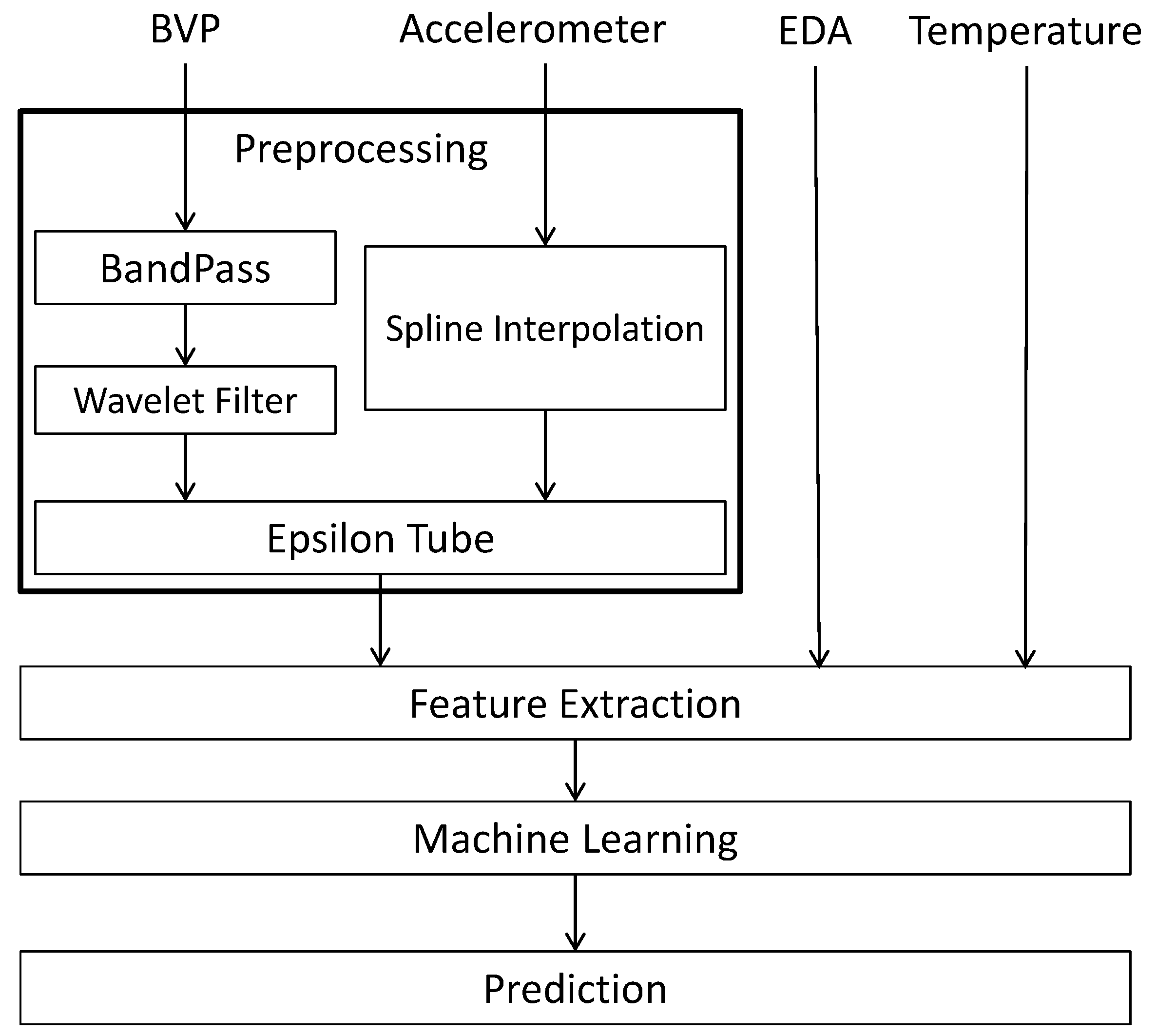
In this study our immediate interest is to predict extreme cases of fatigue and poor sleep in people with fibromyalgia. For such an analysis, we use self-reported quality of sleep and fatigue severity, continuously collected data from the Empatica E4, to measure autonomic nervous system activity during sleep (
Section 2). These signals are preprocessed to remove noise and other artifacts as described in
Section 3.1. After preprocessing, a number of mathematical features are extracted, including various statistics, signal characteristics, and HRV features (
Section 3.2).
Section 4 provides a detailed description of our novel Learning Using Concave and Convex Kernels (LUCCK) machine learning method. This model, along with other conventional machine learning methods, were trained on the extracted features and used to predict extreme cases of poor sleep and fatigue, with our method yielding the best results (
Section 5).
We believe this analytical framework can be readily extended to outpatient monitoring of daytime activity, with applications to assessing extreme levels of fatigue and pain, such as those experienced by patients undergoing chemotherapy.
2. Dataset
The data used for this study was collected from a group of 20 adults with fibromyalgia and consists primarily of a set of signals recorded by an Empatica E4 wristband over the course of seven days (removing 1 h/day for charging/download). Most (80%) participants were female with mean age = 38.79 (min-max = 18–70 years). Of a possible 140 nights of sleep data, the sample had data for 119 (85%) nights. In this dataset, 19.9% of heartbeats were missing due to noisy signals or failure of the Empatica E4 in detecting beats. Data were divided into 5-min windows for HRV analysis; windows with more than 15% missing peaks were eliminated. This led to the exclusion of 30.9% of the windows. The signals used in this analysis are each patient’s blood volume pulse (BVP), 3-axis accelerometer, temperature, and EDA. In addition to these recordings, each subject self-reported his or her wake and sleep times, as well as self-assessed his or her level of fatigue and quality of sleep every morning. These data are labeled by self-reported quality of sleep (1 to 10, 1 being the worst) and level of fatigue (from 1 to 10, 10 indicating the highest level of fatigue).
4. Machine Learning: Learning Using Concave and Convex Kernels
The final step in the analysis pipeline is the creation of a model that can be used to predict the extreme cases of quality of sleep or level of fatigue for people with fibromyalgia. As detailed in
Section 5, in addition to testing a number of conventional machine learning methods, we tested a novel supervised machine learning called Learning Using Concave and Convex Kernels (LUCCK). A key factor in the classification of complex data is the ability of the machine learning algorithm to use vital, feature-specific information to detect settled and complex patterns of changes in the data. The LUCCK method does this by employing similarity functions (defined below) to capture and quantify a model for each of the features separately. The similarity functions are parametrized so that the concavity or convexity of the function within the feature space can be modified as desired. Once the similarity functions and attendant parameters are chosen, the model uses this information to reweight the importance of each feature proportionally during classification.
4.1. Notation
In this section, is a real-valued vector of features such that , and is a real-valued (scalar) feature. Throughout this section, we consider d classes, n features and m (data) samples; also the indexes ; ; and are used for classes, features and samples respectively. Additionally, refers to samples in class .
4.2. Classification Using a Similarity Function
An instructive model for comparison to the Learning Using Concave and Convex Kernels method is the
k-nearest neighbors algorithm [
33,
34,
35] and weighted
k-nearest neighbors algorithm [
36]. In
k-nearest neighbors, a test sample
is classified by comparing it to the
k nearest training samples in each class. This can make the classification sensitive to a small subset of samples. Instead, LUCCK classifies test data by comparing it to
all training data, properly weighted according to their distance to
, which is determined by a similarity function. One major difference between LUCCK and weighted
k-nearest neighbors is that our approach is based on a similarity function that can be highly non-convex. A fat-tailed (relative to a Gaussian) distribution is more realistic for our data, given that there is a small but non-negligible chance that large errors may occur during measurement, resulting in a large deviation in the values of one or more of the features. The LUCCK method allows for large deviations in a few of the features with only a moderate penalty. Methods based on convex notions of similarity or distance (such as the Mahalanobis distance) are unable to deal adequately with such errors.
Suppose that the feature space is comprised of real-valued vectors . A similarity function is a function that measures the closeness of to the origin, and satisfies the following properties:
for all ;
for all ;
if is non-zero and .
The value measures the closeness between the vectors and . Using the similarity function , a classification algorithm can be created as follows:
The set of training data
C is a subset of
and is a disjoint union of
d classes:
. Let
be the cardinality of
C and define
for all
k so that
. To measure the proximity of a feature vector
to a set
Y of training samples, we simply add the contributions of each of the elements in
Y:
A vector
is classified in class
, where
k is chosen such that
is maximal. This classification approach can also be used as the maximum a posteriori estimation (details can be found in
Appendix A).
4.3. Choosing the Similarity Function
The function
has to be chosen carefully. Let
be defined as the product
where
and
only depends on the
i-th feature. The function
is again a similarity function satisfying the properties
for all
, and
whenever
. After normalization, the
can be considered as probability density functions. As such, the product formula can be interpreted as instance-wise independence for the comparison of training and test data. In the naive Bayes method, features are assumed to be independent globally [
37]. Summing over all instances in the training data allows for features to be independent in our model.
Next we need to choose the functions
. One could choose
, so that
is a Gaussian kernel function (up to a scalar). However, this does not work well in practice:
One or more of the features is prone to large errors —The value of is close to 0 even if and only differ significantly in a few of the features. This choice of is therefore very sensitive to small subsets of bad features.
The curse of dimensionality—For the training data to properly represent the probability distribution function underlying the data, the number of training vectors should be exponential in n, the number of features. In practice, it usually is much smaller. Thus, if is a test vector in class , there may not be a training vector in for which is not small.
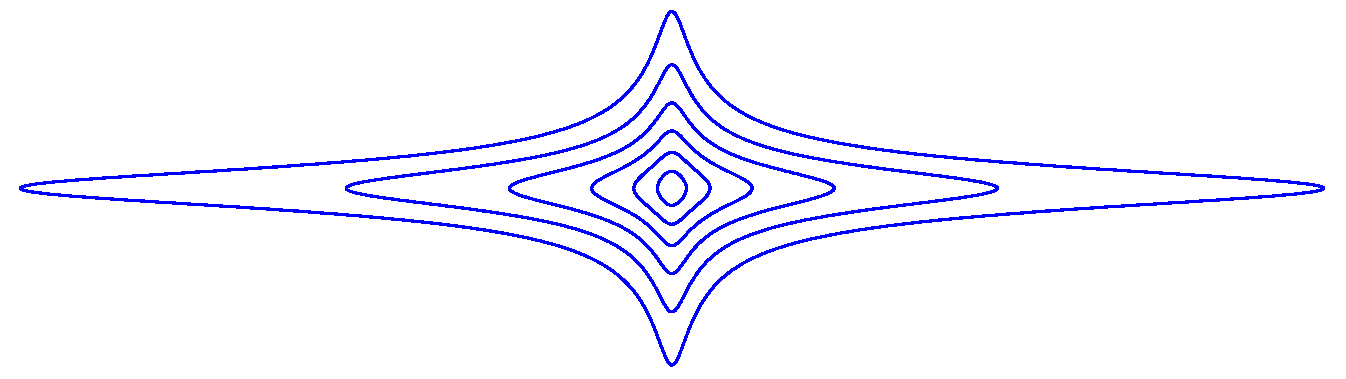
Consequently, let
for some parameters
. The function
can behave similarly to the Cauchy distribution. This function has a “fat tail": as
the rate that
goes to 0 is much slower than the rate at which
goes to 0. We have
The function
Q has a finite integral if
for all
i, though this is not required. Three examples of this function can be found in
Appendix B.
4.4. Choosing the Parameters
Values for the parameters
and
must be chosen to optimize classification performance. The value of
is the most sensitive to changes in
x when
is maximal. An easy calculation shows that this occurs when
. Since the value
directly controls the wideness of
’s tail, it is reasonable to choose a value for
that is close to the standard deviation of the
i-th feature. Suppose that the set of training vectors is
where
for all
j.
Let
, where
be the standard deviation of the
i-th feature. Let
where
is some fixed parameter.
Next we choose the parameters
. We fix a parameter
that will be the average value of
. If we use only the
i-th feature, then we define
for any set
Y of feature vectors. For
in the class
,
gives the average value of
over
. The quantity
measures how much closer
is to samples in the class
than to vectors in the set
C of all feature vectors except
itself. This value measures how well the
i-th feature can classify
as lying in
as opposed to some other class. If we sum over all
and ensure that the result is non-negative we obtain
The
can be chosen so that they have the same ratios as
and sum up to
:
In terms of complexity, if n is the number of features and m is the number of training samples then the complexity of the proposed method would be .
4.5. Reweighting the Classes
Sometimes a disproportionate number of test vectors are classified as belonging to a particular class. In such cases one might get better results after reweighting the classes. The weights
can be chosen so that all are greater than or equal to 1. If
p is a probability vector, then we can reweight it to a vector
where
If the output of the algorithm consists of the probability vectors
the algorithm can be modified so that it yields the output
. A good choice for the weights
can be learned by using a portion of the training data. To determine how well a
training vector
can be classified using the remaining training vectors in
, we define
The value
is an estimate for the probability that
lies in the class
, based on all feature vectors in
C except
itself. We consider the effect of reweighting the probabilities
, by
If
lies in the class
, then the quantity
measures how badly
is misclassified if the reweighting is used. The total amount of misclassification is
We would like to minimize this over all choices of
. As this is a highly nonlinear problem, making optimization difficult, we instead minimize
instead. This minimization problem can be solved using linear programming, i.e., by minimizing the quantity
for the variables
and new variables
under the constraints that
and
for all
k and
j with
and
.
6. Conclusions and Discussion
In this study we primarily focused on prediction of the extreme cases of fatigue and poor sleep. As such, we have created preprocessing/conditioning methods that have the ability to improve the quality of parts of the signals with low quality due to motion artifact and noise. In addition, we identified a set of mathematical features that are important in extracting patterns from physiological signals that can distinguish poor and good clinical outcomes for applications such as fibromyalgia. Additionally, we showed that our proposed machine learning method outperformed the standard methods in predicting the outcomes such as fatigue and sleep quality. Generally, our proposed framework (preprocessing, mathematical features, and proposed machine learning method) can be employed in any study that involves prediction using BVP, HRV and EDA signals.
The epsilon tube filter is covered by US Patent 10,034,638, for which Kayvan Najarian is a named inventor.

 ,
, 


