Understanding of Various Type of Unambiguous Discrimination in View of Coherence Distribution


1
School of Applied Mathematics, National Research University Higher School of Economics, 101000 Moscow, Russia
2
Department of Applied Physics, Hanyang University, Ansan, Kyunggi-Do 425-791, Korea
*
Author to whom correspondence should be addressed.
Entropy 2020, 22(12), 1422; https://doi.org/10.3390/e22121422
Submission received: 16 November 2020
/
Revised: 11 December 2020
/
Accepted: 12 December 2020
/
Published: 16 December 2020
(This article belongs to the Special Issue Foundations of Quantum Mechanics and Quantum Information Theory)
Abstract
:Unambiguous quantum state discrimination is a strategy where the conclusive result can always be trusted. This strategy is very important, since it can be used for various quantum information protocols, including quantum key distribution. However, in the view of quantumness, it is not clear what is going on in performing unambiguous quantum state discrimination. To answer the question, we investigate coherence distribution when unambiguous discrimination is performed by generalized measurement. Specially, we study coherence distribution in three cases, which consist of unambiguous quantum state discrimination, sequential quantum state discrimination, and assisted optimal discrimination, which are considered to be a family of unambiguous quantum state discrimination. In this investigation, we show that the structure of generalized measurements performing various types of unambiguous quantum state discrimination can be understood in terms of coherence distribution. Our result is not limited to the discrimination of two pure quantum states, but it is extended to the discrimination of two mixed states.
1. Introduction
Unambiguous quantum state discrimination (UD) is a strategy for discriminating quantum states without an error. The errorless results in UD require of containing the inconclusive result. Even though many successful applications of UD have been known, it is not clear what can make UD successful. It is known that UD can be constructed in terms of generalized measurement [1,2,3,4,5,6,7]. Because generalized measurement performing UD should consist of preparing an auxiliary(or ancilla) system and interacting with a given quantum system [8,9], understanding what is going on in the interaction of UD is very important.
One can regard UD as a game between a sender called Alice and a receiver called Bob. When the interaction is terminated, there can be many choices for Bob in generalized measurement, according to whether Bob’s measurement is optimal or not and which systems Bob measures on. The first choice is that Bob only performs a local projective measurement on his auxiliary system. If Bob performs non-optimal unambiguous discrimination, which means that Bob’s measurement does not optimize average success probability, then one can obtain partial information from Bob’s post-measurement state [10]. It leads to sequential state discrimination (SSD) [10,11,12,13,14,15,16,17,18]. The second choice is that Bob performs local projective measurement on both Alice and his system. This choice leads to assisted optimal state discrimination (AOSD) [19,20,21,22]. In fact, AOSD is classified into two cases, such as AOSD1 and AOSD2. In AOSD1, Bob discriminates one out of Alice’s two quantum states. Meanwhile, in AOSD2, Bob discriminates every Alice’s quantum state.
Quantum coherence [23] is an important feature in revealing the quantum nature of a system. It is known to help us to understand the concept of wave-particle duality [24,25,26]. Not only that, it is suggested that quantum coherence can be related to a various quantum information processings [27,28,29,30,31]. Additionally, quantum coherence has an advantage in that it can be studied in a single system as well as in a multipartite system. Further, it can be used to unify various quantum characteristics. Additionally, it can help to understand the behavior of quantum operation [32].
Therefore, in this work, using coherence, we study what is going on when the generalized measurement is performed for various types of UD. To do it, we investigate how coherence is distributed in performing generalized measurements for UD, SSD, and AOSD. For the purpose, we consider relative quantum coherence (RQC), as a coherence measure [33]. Further, in order to understand the behavior of coherence distribution, we need to study the localization of relative quantum coherence (RQC). For the measure of localization of relative quantum coherence (RQC), we consider entropic quantum discord [34,35,36,37,38,39,40] and symmetrized discord [11,15].
Our investigation tells that the unitary operator in generalized measurement for UD moves the localization of RQC in Alice’s initial ensemble(or average state) into Bob’s auxiliary system. Meanwhile, the unitary operator in generalized measurement for SSD distributes RQC in Alice’s initial ensemble to both Alice’s and Bob’s systems. Further, the unitary operator in generalized measurement for AOSD1 moves the localization of RQC in Alice’s initial ensemble into Bob’s auxiliary system. Meanwhile, the unitary operator in generalized measurement for AOSD2 distributes RQC in Alice’s initial ensemble to both Alice’s and Bob’s systems.
In an operational view, our result implies that coherence distribution depends on the way where Bob constructs his generalized measurement. As known, UD, SSD, AOSD1, and AOSD2 performs unambiguous discrimination. Because coherence is regarded as a resource for quantum operation, understanding how coherence distribution occurs in these scenarios is an important subject of investigation. We show that the feature of coherence distribution in these scenarios depends on the characteristic of each scenario’s measurement. Further, we show that our argument could be extended to cases, including two mixed states. In other words, our arguments listed above is not limited to discrimination of two pure states. In terms of entropic quantum discord and symmetrized discord as witnesses of RQC localization, our result can help to understand the quantum correlations.
Furthermore, our result consistently reveals a relation between quantumness and unambiguous quantum state discrimination. It is well known that AOSD requires partially quantum dissonance, which is defined as quantum discord in separable state [41]. Meanwhile, our result explains the relationship between coherence distribution and AOSD. Additionally, it should be noted that we could extend our argument successfully to two mixed states case.
This paper is organized. as follows. In Section 2, we briefly review RQC and RQC localization. Additionally, we show that entropic quantum discord and symmetrized discord can be applied for witnesses of RQC localization. In Section 3, we explain four strategies (UD, SSD, AOSD1, and AOSD2), which can be understood as a deformed structure of UD. (Actually, AOSD1 and AOSD2) have an equivalent structure as AOSD. In Section 4, we analyze coherence distribution in generalized measurements for four cases when every two quantum state of Alice is pure. In Section 5, we extend our argument in Section 4 to mixed states case. Finally, we conclude and discuss our result in Section 6. Because UD based algorithms can be applied to quantum random number generation [42], quantum key distribution [43,44], and quantum state tomography [45], our result can contribute to understanding how coherence distribution is essential in quantum information protocols.
2. Preliminaries
2.1. Definition of RQC
Although superposition is one of the fundamental concepts in quantum physics, it is difficult to rigorously define the notion of superposition. Despite this, the state of a system without superposition is expressed as a classical probability distribution, which is equivalent to the diagonal density operator. This state is known as the incoherent state. Additionally, the incoherent operation is defined as a completely positive map (CP map), which maps the set of incoherent state onto itself. In this way, coherence can be defined as a quantity in which incoherent operation does not increase.
From this, the mathematical conditions of coherence measure can be provided, as follows [23]:
- (C1) Assume that is the set of incoherent states. Then, if and only if .
- (C2) Assume that incoherent operation is expressed as a set of Kraus operators .
- −Given the incoherent CPTP map, C satisfies , where .
- −For the post-measurement state and the corresponding probability , C satisfies .
- (C3) C is convex, meaning that C satisfies .
According to Baumgratz, Cramer, and Plenio [23], the relative entropy of coherence satisfies the above three conditions and it is defined as
Example 1.
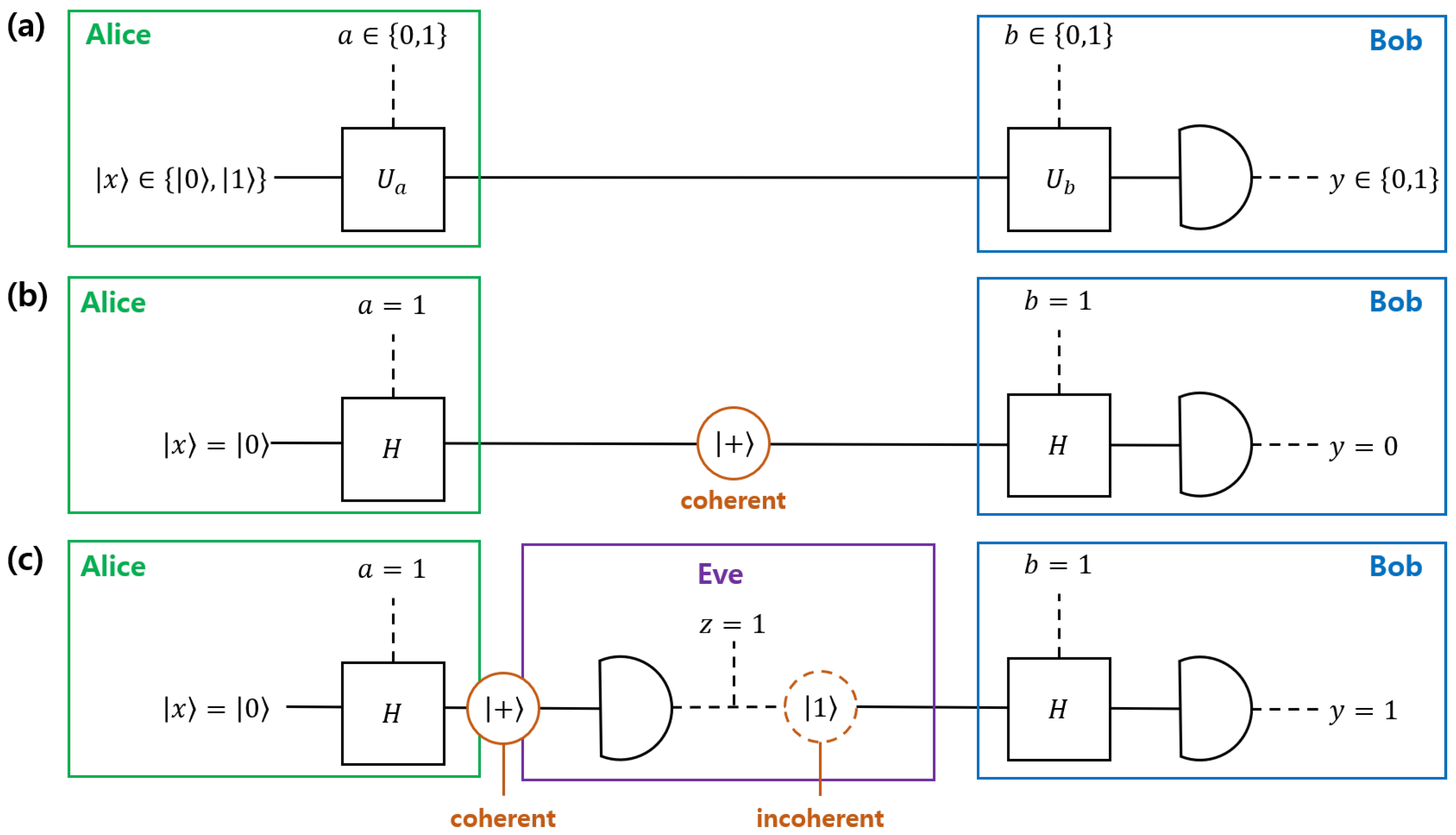
(Role of coherence in BB84 protocol) Most of quantum key distribution protocol uses a superposed state as an information carrier, which has nonzero coherence, in order to provide security between a sender and a receiver. Here, we introduce a BB84 protocol [43], which is described in Figure 1. In Figure 1a, Alice produces a qubit , and performs a unitary operator , depending on her random bit . Here, is an identity if and a Hadamard gate if . Subsequently, Alice sends one out of four qubits . After Alice sends a qubit to Bob, Bob performs a unitary operator , depending on his random bit . Here, is an identity if and a Hadamard gate if . Subsequently, Bob performs a projective measurement and obtains a measurement outcome of .
We assume that a and b are randomly choosen as and , as in Figure 1b. Additionally, we assume that Alice prepares a qubit . Subsequently, Alice’s unitary operator transforms into , which has nonzero coherence in the fixed basis . Because Bob’s unitary operator transforms into , Bob always obtains the measurement outcome of , when Alice prepares .
In Figure 1c, Eve performs eavesdropping between Alice and Bob. Here, we assume that Eve performs a strategy that, after performing her measurement, she sends the qubit corresponding to the measurement outcome of to Bob. Note that Eve’s post-measurement state can be incoherent. Subsequently, there is a possibility that Bob obtains a measurement outcome of , which is different from . Thus, Alice and Bob can notice Eve’s presence by comparing their list of a and b.
Consequently, it implies that coherence can be a resource for security of BB84.
Additionally, M.-L. Hu and H. Fan [33] defined the basis-dependent measure of coherence as
where is a fixed basis, consisting of . This coherence measure is also known as the relative quantum coherence(RQC). If is degenerate, then the basis that consists of is not unique [33]. Therefore, the suprenum of the RQC under every basis of is considered to be
This measure of coherence is also called the maximum RQC [33]. It is well known that RQC is applicable for bipartite system, where it can be related to various quantum correlations, including quantum discord, measurement-induced disturbance, and nonlocality. Particularly, entropic quantum discord has a close relationship with RQC localization.
2.2. Definition of RQC Discrepancy and Localization
In order to define the RQC of a bipartite state , the construction of a fixed basis for systems A and B is required. Assume that both the fixed orthonormal basis and consist of each system A and B. The incoherent state , which corresponds to , is then given as . Likewise, the incoherent state (), which corresponds to the partial state (), is given as (). Therefore, the RQCs of the states , , and are defined as [33]
Because RQC is not increased under the trace out, must be greater than or equal to both and . From an operational viewpoint, not every bipartite system is guaranteed to be localized into a certain subsystem localized. In order to deal with this argument quantitively, the nonlocalized quantities of RQC are defined as
() is also known as the RQC discrepancy. If () is equal to zero, is equal to (). This means that the RQC of is localized into system A(B). However, if () is nonzero, then the RQC of is not localized into system A(B).
2.3. Entropic Quantum Discord as a Witness of RQC Localization
According to a study that was scarried out by M.-L. Hu and H. Fan [33], the discrepancy in the RQC is lower bounded by entropic quantum discord [34]
where and describe the entropic quantum discord, which is defined as
Here, is the von Neumann mutual information between systems A and B. Additionally, () is the classical part of the mutual information between system A and B, where the local measurement that is expressed as POVM () is performed on system A(B) [46]. Equation (1) implies that entropic quantum discord is applicable as a witness for RQC localization. If the entropic quantum discord () is nonzero, then the RQC of is not localized into system A(system B).
The witness in Equation (1) is asymmetric under a change in the lower index. In order to investigate RQC localization, the witness for system A and B should be simultaneously tested. Hence, if a witness is symmetrical under a change in the lower index, we can simultaneously investigate the RQC localization by testing one witness. Fortunately, symmetrized discord can be exploited [11]:
If is nonzero, the RQC of is not localized into A or B. Moreover, if the RQC of is localized into either system A or B, the symmetrized discord is equal to zero. Hence, the symmetrized discord can be applied as a witness in a similar that is manner to symmetric discord [33].
Example 2.
(RQC localization during CNOT operation) By using the formula that is proposed in Ref. [36], the entropic quantum discord of the maximally entangled state is evaluated as . Therefore, the symmetrized discord is nonzero. This implies that RQC of the maximally entangled state is not localized in either the system A or the system B. Additionally, the RQC of the maximally entangled state is , where the fixed basis is and is .
After CNOT operation, the composite state is transformed into . Because this state is a product state, the entropic quantum discord is zero. This implies that the RQC is localized in either the system A or the system B. Because the RQC of the system A is evaluated as , where is a maximally mixed state, we can conclude that the RQC of the maximally entangled state is localized in the system A by the CNOT gate. It implies that RQC localization may be understood as a resource for implementing CNOT operation (Figure 2).
3. Structure of Various Protocols Based on Unambiguous Discrimination
Suppose that unambiguous discrimination is performed by Alice and Bob. Subsequently, one can assume that Alice prepares a pure state , with a prior probability . Here, is not orthogonal to . Alice sends a pure state to Bob through a quantum channel. Subsequently, Bob can discriminate Alice’s pure state without any error. Mathematically, Bob’s measurement is expressed as three elements POVM . Here, is an element that corresponds to a measurement outcome . If , then Bob can conclude that Alice’s pure state is without any error. In this case, the outcome of measurement i is considered as a conclusive outcome. Meanwhile, if , Bob cannot conclude which of Alice’s pure states is prepared. In this case, the measurement outcome is considered as the inconclusive outcome.
If the possibility that Bob obtains an inconclusive outcome is excluded, then Bob cannot carry out the measurement which discriminates Alice’s pure states without an error. This is because nonorthogonal pure states cannot be perfectly discriminated, according to quantum theory.
When the generalized measurement is considered, Bob needs to extend the Hilbert space, where Alice’s pure state resides. If the Hilbert space of Alice (Bob) is denoted as (), the task of generalized measurement should consider a unitary operator , where Alice’s pure state resides in and the state of Bob’s auxiliary system is found in .
After the unitary operator is performed, Bob’s composite state is measured via a projective measurement. Bob then discriminates Alice’s pure states without any error, which is obtained by the projective measurement. The structure of depends on how Bob constructs the projective measurement.
3.1. The Structure of Unambiguous Discrimination (UD) and Sequential State Discrimination (SSD)
First, if Bob only performs a local projective measurement on his ancilla system, the structure of is:
Bob’s local projective measurement is expressed as . The non-negative real value is the probability that Bob obtains the conclusive outcome i, and is the probability that Bob obtains the inconclusive outcome (see Figure 3). A controlled-unitary operator performs and . Therefore, we can consider as , without any loss of generality. Therefore, Equation (3) can also be expressed as
The necessary and sufficient condition for global unitary operator of Equations (3) and (4) can be obtained by the following Lemma [47].
Lemma 1.
Consider two sets and , which consist of finite vectors. For , the necessary and sufficient condition for global unitary operator performing is that for , one has .
Applying this Lemma to Equations (3) and (4), the necessary and sufficient condition for and is given, as follows:
In other words, the strategy of quantum state discrimination when considering Equations (3) and (4) has the identical constraint. This implies that, without losing consistency, one can choose the formalism of Equation (4). (If the post-measurement state of Bob is given by one of the set , then Charlie can discriminate the post-measurement state of Bob without any error. Therefore, the formalism of Equation (4) provides sequential state discrimination (SSD) of Bob and Charlie.)
Suppose that Alice prepares one of two pure states . Here, let us assume that is a real number. Subsequently, the explicit form of is expressed as [11]
Here, , and . is an operator, which acts on the subspace of . This explicitly means that for all . When Equation (5) is satisfied, the structure of provides various explicit forms of two input state and post-measurement states . For instance, an explicit form of can be given by
Afterwards, the explicit form of post-measurement states is provided by
When explicit forms of input states and post-measurement states are provided, is determined. In UD, Bob discriminates pure states of Alice optimally. Therefore, the post-measurement states of Bob are completely overlapped (). According to explicit form of Equation (6), the post-measurement states become , which are identical. (Suppose that . Because there exists an incoherent unitary operator performing , the explicit form of post-measurement states cannot be fixed. In fact, the incoherent unitary operator acts on Alice’s system and it does not affect the optimal success probability and optimal conditions.) This implies that, in UD, the coherence of Alice’s ensemble is localized in Bob’s ancilla system.
In Equation (4), the unitary operator generates a post-measurement state , which corresponds to the measurement outcome i. Therefore, there is a subsequent measurement, which can extract an information from Bob’s post-measurement state, if Bob performs a nonoptimal unambiguous discrimination. If Charlie constructs a subsequent measurement, Alice, Bob and Charlie can perform sequential state discrimination [10]. In this case, Charlie’s measurement includes the unitary operator , which is expressed as
Charlie’s local projective measurement is expressed as . The non-negative real value is the probability that Charlie obtains a conclusive result i, and is the probability that Charlie obtains a inconclusive result. The structure of sequential state discrimination (SSD) consists of in Equation (4) and in Equation (7). The structure of Charlie’s measurement depends on the setting of Bob’s measurement [10]. From Bob’s viewpoint, whether his measurement has structure of UD or SSD depends only on whether he performs an optimal discrimination or not. Because UD does not include Charlie, Bob has to optimally discriminate Alice’s states. However, in SSD, Bob should not perform optimal discrimination. If Bob performs the optimal unambiguous discrimination, then Charlie cannot perform unambiguous discrimination on Bob’s post-measurement states.
3.2. Structure of Assisted Optimal State Discrimination (AOSD)
Second, if Bob performs a projective measurement on both Alice’s system and his own, the unitary operator is in the form [22]
where is the orthonormal basis which consists of and . It is also apparent that . Here, the inner product is expressed as .
Bob performs a local projective measurement on each system (See Figure 4). Here, is the probability that Bob obtains the conclusive result i, and is the probability that Bob obtains the inconclusive result. If Bob obtains a conclusive result “0” by measuring system B, then he can discriminate Alice’s pure state, from the measurement outcome on system A. If the measurement outcome of system A is i, then, without any error, Bob can conclude that Alice’s pure state is . Meanwhile, if Bob obtains the conclusive result “1” by measuring system B, he cannot discriminate Alice’s pure states. Hence, the measurement outcome on system B informs Bob as to whether the measurement outcome is conclusive or not, and the result on system A tells Bob which pure state Alice has prepared.
This structure is known as assisted optimal state discrimination (AOSD). However, every case of AOSD uses both of the local projective measurements. Suppose that Bob discriminates one of Alice’s pure states(in this case, it is called AOSD1). Bob then only needs the measurement outcome on system B. Meanwhile, if Bob discriminates every pure state of Alice (in this case, it is called AOSD2), Bob should consider every measurement outcome.
4. Investigating Coherence Distribution in Various Protocols
4.1. Coherence Distribution in UD and SSD
Because the unitary operators of UD and SSD have the same structure, the coherence distribution of UD and SSD can be analyzed while using the same geometric structure. This geometric structure comes from the necessary and sufficient condition that the unitary operator exists. Because preserves the inner product between two pure states, the necessary and sufficient conditon that exists is expressd as [14,16]
Here, . In Equation (8), it is assumed that, for post-measurement states and , . The set of two-dimensional real vectors , which satisfies Equation (8), can be geometrically expressed, as seen in Figure 5. Here, Bob’s measurement setting has one-to-one correspondence with a real vector . Additionally Bob’s optimal measurement corresponds to a tangential point between the curve and the line (here, is the average success probability of Bob).
In many discrimination strategies, Alice informs Bob of her prior probability distribution. This means that, from the viewpoint of Bob, Alice’s state is expressed as the initial ensemble (or average state) [11,22]. Therefore, the unitary operator will produce an average state, expressed as
In UD, the post-measurement states become identical, which means that . Therefore, is an incoherent state. Meanwhile, in SSD, and are neither orthogonal nor identical. Therefore, has nonzero coherence. Therefore, UD and SSD have a difference in coherence distribution.
Now, let us evaluate coherence distribution of UD and SSD by using measure of coherence. Because Alice’s two pure states are non-orthogonal, the initial ensemble consists of nonzero coherence. Now, we investigate how the unitary operator distributes the coherence of the initial ensemble. First, let us consider the maximum RQC of system B. The maximum RQC of system B is expressed, as [15,33]
Hence, is expressed as a function of . Here, is a function of entropy: , where . According to Equation (9), as becomes closer to , becomes closer to the maximum. This implies that if Bob performs an optimal unambiguous discrimination, then will reach the maximum.
Furthermore, when corresponds to the optimal measurement that exists on curve , two post-measurement states and overlap completely [14,16]. This implies that, in UD, the coherence in Alice’s initial ensemble is localized to Bob’s auxiliary system via unitary operator .
In this time, let us assume that Bob and Charlie perform sequential state discrimination. If vector that correponds to Bob’s measurement is on curve , then Charlie cannot perform unambiguous discrimination. Therefore, the vector should be inside sector . Because the success probability of sequential state discrimination is given as function , the optimal vector always satisfies the equality . We can numerically verify that a vector, satisfying a zero-gradient condition, will always be on curve . Every vector on this curve satisfies:
Next, we investigate symmetrized discord to understand the RQC localization in SSD. Here, entropic quantum discord is derived as [11,15]
Here, the tangles are given as
According to Equation (11) and Equation (12), symmetrized discord is also given as a function of . Therefore, we numerically find an optimal vector that maximizes the symmetrized discord. Consequently, we can see that the optimal vector always exists on a curve . This implies that, in SSD, the coherence in Alice’s initial ensemble is distributed to both system A and B. In other words, the coherence of is localized to neither system A nor B.
Observation 1.
Suppose that Alice prepares one of two pure states. In UD, the unitary operator localizes the coherence in Alice’s initial ensemble into system B. Meanwhile, in SSD, distributes the coherence in Alice’s initial ensemble to both systems A and B.
From Observation 1, we propose that coherence distribution obviously depends on which strategy Bob chooses. If Bob chooses UD, the coherence in the initial ensemble is localized in the ancilla system. If Bob chooses SSD, the coherence in the initial ensemble is not localized in B.
4.2. Coherence Distribution in AOSD1 and AOSD2
Here, we investigate the coherence distribution in the unitary operator , where assisted optimal state discrimination is performed.
The unitary operator transforms Alice’s initial ensemble into the following:
According to Zhang, Chen, Kwek, and Vedral [22], zero concurrence in the average state is analytically expressed as
Because the success probability is not affected by the two parameters and , we can assume that without any loss of generality. and do not affect the success probability. In other words, can be considered as a real number.
Assume that holds. When , Bob’s optimal strategy is described as AOSD2. In this case, is given, as follows [22]:
Here, is provided, as follows:
According to Ref. [22], is nonzero. This implies that the RQC in is not localized in system B. According to structure of , the partial state is an ensemble that is composed of two nonorthogonal pure states. Hence, RQC is not localized in system B.
Meanwhile, if , Bob’s optimal strategy is described as AOSD1. In this case, is given, as follows [22]:
Here, becomes
Clearly, is an incoherent state. Furthermore, is obviously zero, since is a product state. This implies that the RQC in has the potential to be localized in system B. According to Zhang, Chen, Kwek, and Vedral [22], the partial state is given as a pure incoherent state. Therefore, the RQC shown in is obviously localized in system B.
Observation 2.
Suppose that Alice prepares one of two pure states. In AOSD2, the coherence in is not localized in system B. Meanwhile, in AOSD1, the coherence in is localized in system B.
From Observation 2, we can tell that the coherence distribution in AOSD also depends on which strategy Bob chooses. If Bob chooses AOSD2, the coherence is distributed to both system A and B. If Bob chooses AOSD1, the coherence is localized in system B. These results imply that the structure of generalized measurements performing unambiguous discrimination, sequential state discrimination, and assisted optimal state discrimination can be understood by coherence distribution.
Zhang, Chen, Kwek, and Vedral [22] attempted to explain the structure of AOSD in terms of quantum discord (or dissonance) However, if there is significant overlap between two pure states, the entropic quantum discord becomes zero. In other words, the relationship between AOSD and entropic quantum discord holds only when specific constraints concerning overlap are imposed. Meanwhile, According to Figure 6, the RQC of system B is nonzero in the region , where it is assumed that . Therefore, Observation 2 implies that there is a consistent relationship between coherence distribution and AOSD.
5. Generalization of Coherence Distribution to 2 Mixed States Discrimination
Here, let us suppose that Alice prepares a mixed state , with a prior probability . If the support of and do not ovelap completely, then Bob’s measurement can discriminate Alice’s mixed state without any error [49,50]. Additionally, the POVM element () consists of the kernel of (). Unfortunately, the general structure of POVM, which can discriminate a general mixed state without an error, has been unknown yet. However, if Alice’s Hilbert space has a special form in , the structure of POVM for unambiguous discrimination is well known [51]. If we assume that the state space is constructed from this form of Hilbert space, then Alice’s mixed state can be expressed as
Here, R is maximum rank of . If holds for all of , then Bob can discriminate Alice’s mixed states without any error. Fortunately, Bob’s POVM consists of R sub-POVMs, where each sub-POVM discriminates () without any error. This implies that we can consistently substitute our argument of pure states into that of mixed states (the detailed evaluation can be found in Appendix A and Appendix B).
5.1. Generalized Witness of RQC Localization
Now, let us consider . That is, unitary operator maps onto itself. This unitary operator transforms Alice’s initial ensemble into an average state expressed as
Here, is a normalized positive-semidefinite operator. Because every is of rank-2, then the Koashi–Winter formula can be used in order to obtain a lower bound for the entropic quantum discord and symmetrized discord:
Because holds for all of and , the lower bound of the RQC discrepancy in becomes:
5.2. Generalization of Coherence Distribution in UD and SSD
In cases of UD and SSD, unitary operator has the specific form of . Here, is sub-unitary and it is defined as
After is terminated, then Bob’s local projective measurement is performed on system B.
The necessary and sufficient condition that must exist is expressed in a similar manner while using Equation (10). This implies that Bob’s measurement consists of R real vectors . Here, each convex set has the same structure as that seen in Figure 5. Therefore, we can apply our argument of SSD to cases, including mixed states [14].
From the structure of Equation (14), the maximum RQC of is explicitly derived as
If the prior probabilities of the two mixed states and are given as and , respectively, then the entire unambiguous discrimination consists of R discrimination problems, where the pure state is prepared with the prior probability . Hence, tangle is given as
For all of , if is on the boundary of the convex set , the maximum RQC of becomes maximized. Meanwhile, the support between the two post-measurement states is completely overlapped. Therefore, system A does not contain coherence. In conclusion, we can successfully extend Observation 1 to cases of mixed states.
Observation 3.
Suppose that Alice prepares one out of two mixed state. In UD, the unitary operator localizes the coherence in Alice’s initial ensemble into system B. In SSD, distributes the coherence in Alice’s initial ensemble to both system A and B.
5.3. Generalization of Coherence Distribution in AOSD1 and AOSD2
Likewise, the unitary operator also has a specific form of . Here, performs
Here, is an orthonormal basis consisting of . Moreover, . The inner product between two vectors is expressed as . After is terminated, Bob performs the projective measurement on his system.
Likewise, in UD and SSD, in AOSD, maps to itself.
Therefore, we can successfully extend Observation 2 to instances of mixed states.
Observation 4.
Suppose that Alice prepares one out of two mixed states. Subsequently, In AOS12, the coherence of an initial bipartite ensemble is localized in system B. Meanwhile, in an AOSD2, the coherence of in an initial bipartite ensemble is not localized in system B.
6. Conclusions and Future Work
In this paper, we investigated how the distribution of coherence occurs when generalized measurement performs various types of unambiguous discrimination. By investigating the RQC localization, we showed that the coherence distribution depends on the types of quantum unambiguous discrimination (See Figure 7). In other words, we found that the types of quantum unambiguous discrimination determine how coherence is distributed in performing unambiguous discrimination. Further, we showed that our argument could be extended to cases, including two mixed states.
In fact, generalized measurement can be applied to performing not only unambiguous discrimination, but also minimum error discrimination [52,53,54,55,56,57,58] and the fixed rate of inconclusive result [59,60]. Therefore, while using the argument provided in this work, it is interesting to investigate whether coherence distribution can explain the structure of generalized measurements performing other quantum state discriminations. In other words, it can be important to study coherence distribution in various quantum state discrimination strategies.
Beyond the discrimination tasks, a generalized measurement can be applied to various quantum information and computation tasks. The quantum classifier [32], whose efficiency is given as for the number of data N, can be a good example. In training a quantum classifier, which is composed of (a), a parametric multilayer quantum circuit performed on both feature register and index register (b) local projective measurements performed on index register, it is shown that the successfully trained parametric multilayer quantum circuit distributes coherence in the index register [61]. It can be understood that, in the generalized measurement of the problem, the measurement on the index register is important. Further, in the quantum classifier, the Grover algorithm depletes the index register’s coherence as a resource [28,30]. Therefore, investigating coherence distribution in generalized measurement may provide a clue for quantum advantage in quantum tasks.
Author Contributions
Conceptualization, M.N. and Y.K.; Methodology, M.N.; Investigation, M.N.; Software, M.N.; Writing–first draft, M.N. and Y.K.; Revision, Y.K. All authors have read and agreed to the published version of the manuscript.
Funding
This work is supported by the Basic Science Research Program through the National Research Foundation of Korea funded by the Ministry of Education, Science and Technology (NRF2018R1D1A1B07049420) and Institute of Information & communications Technology Planning & Evaluation(IITP) grant funded by the Korea government(MSIT) (No.2020001343, Artificial Intelligence Convergence Research Center (Hanyang University ERICA)).
Conflicts of Interest
The authors declare no conflict of interest.
Appendix A. Deriving the Relationship between Discord and Generalized Witness in the Case of Two Mixed States
Firstly, the rank-2 state is considered to be
Although we consider the case in which the states are rank-2, our method can be extended to the rank-N states case. Obviously, the bipartite state resides in state space . Here, let us consider the entropic quantum discord . Since Equation (A1) is decomposed as a direct sum between the two rank-2 positive semidefinite operator, POVM can also be expressed as
Here, () is a positive semidefinite operator defined over Hilbert space () and () is a linear map in which ().
As is positive semidefinite, is also positive semidefinite for all . Obviously, and are also elements of . Here, () is zero vector in sub Hilbert space (). Thus, and are also positive semidefinite for all and . In other words, if is positive semidefinite, then and are also positive semidefinite.
The completeness of two sub-POVMs is directly checked as
Here, is the null operator. is an identity operator over Hilbert space . () is an identity operator over Hilbert space (). Therefore, if , then the equalities automatically hold. Without loss of generality, we can assume that every nonzero operator satisfies . That is, because the explicit form of does not affect the expression for the lower bound of quantum discord. Therefore, two sub-POVMs and also satisfy completeness condition.
Using concavity of von Neumann entropy, we derive the inequality of conditional entropy as
Here, we define and as and :=.
In order that the quantum discord is evaluated, we minimize the conditional entropy under every POVM [34]. Since POVM element consists of and , the minimum conditional entropy satisfies
As and are independent on , conditional entropy is also independent on . Therefore, the second equality holds. Inequality can be derived from the convexity of von Neumann entropy. We apply the Koashi-Winter formula [48] to final expression. The purification of and is expressed as
Here, () is orthonormal basis constructing system E(system ). According to the Koashi-Winter formula, we can derive the inequality as [11,15]
where is entanglement of formation [62]. We can easity derive the equality . Hence, we obtain the inequality:
A.2 Deriving the relationship between discord and generalized witness Likewise, we can obtain the expression for and as
Here, is decomposed as direct sum between the two positive semidefinite operators. Therefore, von Neumann entropy satisfies
Hence, conditional entropy satisfies
Also, minimum of conditional entropy also satisfies
This inequality consists of two optimization problems (Problem I and Problem II). The Problem I contains additional equality constraint , but this constraint is not included in the Problem II. Therefore, minimum of the Problem I is not smaller than that of the Problem II. Finally, we obtain the lower bound of quantum discord as
A.3 Deriving the relationship between discord and generalized witness .
In this case, derivation is more straightforward. Substituting and into , we obtain
In second inequality, the Cauchy Schwarz inequality is used: (for all real vectors ).
Appendix B. Deriving the Generalized RQC Discrepancy
In this Appendix, we derive the generalized RQC discrepancy. Two positive semidefinite operators and in Equation (A1) are defined over sub-Hilbert space and . Therefore, the entire Hilbert space consists of orthonormal basis and . Here, sub-Hilbert space () is composed of (). Using this property of Hilbert space, we can evaluate von Neumann entropy of the incoherent state as [33]
Also, the RQC of is evaluated as
Next, we evaluate the RQC of system A and B. First, we consider the partial state :
As the supports of and are orthogonal, von Neumann entropy of is expressed as
As the partial state is given as , von Neumann entropy of is also expressed as
Therefore, the RQC of system A is derived as
Finally, we derive generalized RQC discrepancy as
In a similar manner, the generalized RQC discrepancy is also derived as
References
- Ivanovic, I.D. How to differentiate between non-orthogonal states. Phys. Lett. A 1987, 123, 257. [Google Scholar] [CrossRef]
- Dieks, D. Overlap and distinguishability of quantum states. Phys. Lett. A 1988, 126, 303. [Google Scholar] [CrossRef]
- Peres, A. How to differentiate between non-orthogonal states. Phys. Lett. A 1988, 128, 19. [Google Scholar] [CrossRef]
- Jaeger, G.; Shimony, A. Optimal distinction between two non-orthogonal quantum states. Phys. Lett. A 1995, 197, 83. [Google Scholar] [CrossRef]
- Pang, S.; Wu, S. Optimum unambiguous discrimination of linearly independent pure states. Phys. Rev. A 2009, 80, 052320. [Google Scholar] [CrossRef] [Green Version]
- Bergou, J.A.; Futschik, U.; Feldman, E. Optimal Unambiguous Discrimination of Pure Quantum States. Phys. Rev. Lett. 2012, 108, 250502. [Google Scholar] [CrossRef] [PubMed] [Green Version]
- Ha, D.; Kwon, Y. Analysis of optimal unambiguous discrimination of three pure quantum states. Phys. Rev. A 2015, 91, 062312. [Google Scholar] [CrossRef]
- Nielson, M.A.; Chuang, I.L. Quantum Computation and Quantum Information: 10th Anniversary Edition; Cambridge University Press: Cambridge, UK, 2010. [Google Scholar]
- Zhou, X.-F.; Liu, Q.; Zheng, Y.-S.; Guo, G.-C. Physical accessible transformation on a finite number of quantum states. Phys. Rev. A 2007, 75, 012321. [Google Scholar] [CrossRef] [Green Version]
- Bergou, J.A.; Feldman, E.; Hillery, M. Extracting Information from a Qubit by Multiple Observers: Towards a Theory of Sequential State Discrimination. Phys. Rev. Lett. 2013, 111, 100501. [Google Scholar] [CrossRef] [Green Version]
- Pang, C.-Q.; Zhang, F.-L.; Liang, M.-L. Sequential state discrimination and requirement of quantum dissonance. Phys. Rev. A 2013, 88, 042331. [Google Scholar] [CrossRef] [Green Version]
- Solis-Prosser, M.A.; Gonzalez, P.; Fuenzalida, J.; Gomez, S.; Xavier, G.B.; Delgado, A.; Lima, G. Experimental multiparty SSD. Phys. Rev. A 2016, 94, 042309. [Google Scholar]
- Hillery, M.; Mimih, J. Sequential discrimination of qudits by multiple observers. J. Phys. A Math. Theor. 2016, 50, 435301. [Google Scholar] [CrossRef] [Green Version]
- Namkung, M.; Kwon, Y. Optimal sequential state discrimination between two mixed quantum states. Phys. Rev. A 2017, 96, 022318. [Google Scholar] [CrossRef]
- Zhang, J.-H.; Zhang, F.-L.; Liang, M.-L. Sequential state discrimination with quantum correlation. Quant. Inf. Process. 2018, 17, 260. [Google Scholar] [CrossRef] [Green Version]
- Namkung, M.; Kwon, Y. Analysis of Optimal Sequential State Discrimination for Linearly Independent Pure Quantum States. Sci. Rep. 2018, 8, 6515. [Google Scholar] [CrossRef] [PubMed] [Green Version]
- Namkung, M.; Kwon, Y. Sequential state discrimination of coherent states. Sci. Rep. 2018, 8, 16915. [Google Scholar] [CrossRef] [PubMed] [Green Version]
- Namkung, M.; Kwon, Y. Generalized sequential state discrimination for multiparty QKD and its optical implementation. Sci. Rep. 2020, 10, 8247. [Google Scholar] [CrossRef]
- Li, B.; Fei, S.-M.; Wang, Z.-X.; Fan, H. Assisted state discrimination without entanglement. Phys. Rev. A 2012, 85, 022328. [Google Scholar] [CrossRef] [Green Version]
- Roa, L.; Retamal, J.C.; Alid-Vaccarezza, M. Dissonance is Required for Assisted Optimal State Discrimination. Phys. Rev. Lett. 2011, 107, 080401. [Google Scholar] [CrossRef]
- Xu, L.F.; Zhang, F.L.; Liang, M.L.; Chen, J.L. Assisted optimal state discrimination without entanglement. EPL 2014, 106, 50004. [Google Scholar] [CrossRef] [Green Version]
- Zhang, F.-L.; Chen, J.-L.; Kwek, L.C.; Vedral, V. Requirement of Dissonance in Assisted Optimal State Discrimination. Sci. Rep. 2013, 3, 2134. [Google Scholar] [CrossRef] [PubMed] [Green Version]
- Baumgratz, T.; Cramer, M.; Plenio, M.B. Quantifying Coherence. Phys. Rev. Lett. 2014, 113, 140401. [Google Scholar] [CrossRef] [PubMed] [Green Version]
- Bera, M.N.; Qureshi, T.; Siddiqui, M.A.; Pati, A.K. Duality of quantum coherence and path distinguishability. Phys. Rev. A 2015, 92, 012118. [Google Scholar] [CrossRef] [Green Version]
- Bagan, E.; Bergou, J.A.; Cottrell, S.S.; Hillery, M. Relations between Coherence and Path Information. Phys. Rev. Lett. 2016, 116, 160406. [Google Scholar] [CrossRef] [Green Version]
- Bagan, E.; Calsamiglia, J.; Bergou, J.A.; Hillery, M. Duality Games and Operational Duality Relation. Phys. Rev. Lett. 2018, 120, 050402. [Google Scholar] [CrossRef] [PubMed] [Green Version]
- Hillery, M. Coherence as a resource in decision problems: The Deutsch-Jozsa algorithm and a variation. Phys. Rev. A 2016, 93, 012111. [Google Scholar] [CrossRef] [Green Version]
- Shi, H.-L.; Liu, S.-Y.; Wang, X.-H.; Yang, W.-L.; Yang, Z.-Y.; Fan, H. Coherence depletion in the Grover quantum search algorithm. Phys. Rev. A 2017, 95, 032307. [Google Scholar] [CrossRef] [Green Version]
- Pan, M.; Qiu, D. Operator coherence dynamics in Grover’s quantum search algorithm. Phys. Rev. A 2019, 100, 012349. [Google Scholar] [CrossRef]
- Liu, Y.-C.; Shang, J.; Zhang, X. Coherence Depletion in Quantum Algorithms. Entropy 2019, 21, 260. [Google Scholar] [CrossRef] [Green Version]
- Ma, J.; Hakande, A.; Yuan, X.; Ma, X. Coherence as a resource for source-independent quantum random-number generation. Phys. Rev. A 2019, 99, 022328. [Google Scholar] [CrossRef] [Green Version]
- Namkung, M.; Kwon, Y. Coherence and Entanglement Dynamics in Training Quantum Perceptron. Entropy 2020, 22, 1277. [Google Scholar] [CrossRef] [PubMed]
- Hu, M.-L.; Fan, H. Relative quantum coherence, incompatibility, and quantum correlations of states. Phys. Rev. A 2017, 95, 052106. [Google Scholar] [CrossRef] [Green Version]
- Ollivier, H.; Jurek, W.H. Quantum Discord: A Measure of The Quantumness of Correlation. Phys. Rev. Lett. 2001, 88, 017901. [Google Scholar] [CrossRef] [PubMed]
- Hamieh, S.; Kobes, R.; Zaraket, H. Positive-operator-valued measure optimization of classical correlations. Phys. Rev. A 2004, 70, 052325. [Google Scholar] [CrossRef]
- Luo, S. Quantum discord for two-qubit systems. Phys. Rev. A 2008, 77, 042303. [Google Scholar] [CrossRef]
- Ali, M.; Rau, A.R.P.; Alber, G. Quantum discord for two-qubit X states. Phys. Rev. A 2010, 82, 042105. [Google Scholar] [CrossRef] [Green Version]
- Chen, Q.; Zhang, C.; Yu, S.; Yi, X.X.; Oh, C.H. Quantum discord of two-qubit X states. Phys. Rev. A 2011, 84, 042313. [Google Scholar] [CrossRef] [Green Version]
- Huang, Y. Quantum discord for two-qubit X states: Analytical formula with very small worst-case error. Phys. Rev. A 2013, 88, 014302. [Google Scholar] [CrossRef] [Green Version]
- Namkung, M.; Chang, J.; Shin, J.; Kwon, Y. Revisiting Quantum Discord for Two-Qubit X States: The Error Bound to an Analytical Formula. Int. J. Theor. Phys. 2015, 54, 3340. [Google Scholar] [CrossRef] [Green Version]
- Modi, K.; Paterek, T.; Son, W.; Vedral, V.; Williamson, M. Unified View of Quantum and Classical Correlations. Phys. Rev. Lett. 2010, 104, 080501. [Google Scholar] [CrossRef] [Green Version]
- Brask, J.B.; Martin, A.; Esposito, W.; Houlmann, R.; Bowles, J.; Zbinden, H.; Brunner, N. Megahertz-Rate Semi-Device-Independent Quantum Random Number Generators Based on Unambiguous State Discrimination. Phys. Rev. Appl. 2017, 7, 054108. [Google Scholar] [CrossRef]
- Bennett, C.H.; Brassard, G. Quantum cryptography: Public Key distribution and coin tossing. In Proceedings of the International Conference on Computers, Systems and Signal Processing, Bangalore, India, 9–12 December 1984. [Google Scholar]
- Bennett, C.H. Quantum Cryptography Using Any Two Nonorthogonal States. Phys. Rev. Lett. 1992, 68, 3121. [Google Scholar] [CrossRef]
- Ha, D.; Kwon, Y. A minimal set of measurements for qudit-state tomography based on unambiguous discrimination. Quant. Inf. Process. 2018, 17, 232. [Google Scholar] [CrossRef]
- Henderson, L.; Vedral, V. Classical, quantum and total correlations. J. Phys. A Math. Gen. 2001, 34, 6899. [Google Scholar] [CrossRef]
- Duan, L.-M.; Guo, G.-C. Probabilistic cloning and identification of linearly independent quantum states. Phys. Rev. Lett. 1998, 80, 4999. [Google Scholar] [CrossRef] [Green Version]
- Koashi, M.; Winter, A. Monogamy of quantum entanglement and other correlations. Phys. Rev. A 2004, 69, 022309. [Google Scholar] [CrossRef] [Green Version]
- Rudolph, T.; Spekken, R.W.; Turner, P.S. Unambiguous discrimination of mixed states. Phys. Rev. A 2003, 68, 010301. [Google Scholar] [CrossRef] [Green Version]
- Raynal, P.; Lutkenhaus, N.; van Enk, S.J. Reduction theorems for optimal unambiguous state discrimination of density matrices. Phys. Rev. A 2003, 68, 022308. [Google Scholar] [CrossRef] [Green Version]
- Herzog, U. Optimum unambiguous discrimination of two mixed states and application to a class of similar states. Phys. Rev. A 2007, 75, 052309. [Google Scholar] [CrossRef] [Green Version]
- Helstrom, C.W. Quantum Detection and Estimation Theory; Academy Press: New York, NY, USA, 1976. [Google Scholar]
- Bae, J. Structure of minimum-error quantum state discrimination. New J. Phys. 2013, 15, 073037. [Google Scholar] [CrossRef] [Green Version]
- Ha, D.; Kwon, Y. Complete analysis of three-qubit mixed-state discrimination. Phys. Rev. A 2013, 87, 062302. [Google Scholar] [CrossRef] [Green Version]
- Ha, D.; Kwon, Y. Discriminating N-qudit states using geometric structure. Phys. Rev. A 2014, 90, 022330. [Google Scholar] [CrossRef]
- Namkung, M.; Kwon, Y. Almost minimum error discrimination of N-ary weak coherent states by Jaynes-Cummings Hamiltonian dynamics. Sci. Rep. 2019, 9, 19664. [Google Scholar] [CrossRef] [PubMed] [Green Version]
- Kim, J.; Ha, D.; Kwon, Y. Uniqueness of Minimax Strategy in View of Minimum Error Discrimination of Two Quantum States. Entropy 2019, 21, 671. [Google Scholar] [CrossRef] [PubMed] [Green Version]
- Han, R.; Leuchs, G.; Bergou, J.A. The Helstrom measurement: A nondestructive implementation. Phys. Rev. A 2020, 101, 032103. [Google Scholar] [CrossRef] [Green Version]
- Ha, D.; Kwon, Y. An optimal discrimination of two mixed qubit states with a fixed rate of inconclusive results. Quant. Inf. Process. 2017, 16, 273. [Google Scholar] [CrossRef] [Green Version]
- Zhang, W.-H.; Ren, G. State discrimination of two pure states with a fixed rate of inconclusive answer. J. Mod. Opt. 2018, 65, 192. [Google Scholar] [CrossRef]
- Du, Y.; Hsieh, M.-H.; Liu, T.; Tao, D. Implementable Quantum Classifier for Nonlinear Data. arXiv 2018, arXiv:1809.06056. [Google Scholar]
- Wootters, W.K. Entanglement of formation of an arbitrary state of two qubits. Phys. Rev. Lett. 1998, 80, 2245. [Google Scholar] [CrossRef] [Green Version]
Figure 1.
Description of BB84 protocol and coherence therein. In (a), Alice prepares a qubit , and Bob performs a projective measurement . Here, Alice (Bob) performs a unitary operator (), depending on a random bit (). Here, is an identity if , and is a Hadamard if . In (b), we assume that Alice prepares , and a is given as . Subsequently, transforms into , which has nonzero coherence. If , Bob obtains a measurement outcome which is same as . In (c), Eve appears between Alice and Bob. Eve uses a strategy to measure Alice’s qubit and sends , which corresponds to her outcome z, to Bob. Suppose that and . Subsequently, Eve’s operation can be incoherent, since it transforms the coherent state into the noncoherent state, on a fixed basis. Because of this, there is a possibility that Bob obtains , even if .

Figure 2.
Relative quantum coherence (RQC) localization in CNOT operation. When the input is a maximally entangled state , RQC of it is not localized in either a system A or a system B. However, after the CNOT operation, the RQC is localized in a system A.
Figure 2.
Relative quantum coherence (RQC) localization in CNOT operation. When the input is a maximally entangled state , RQC of it is not localized in either a system A or a system B. However, after the CNOT operation, the RQC is localized in a system A.

Figure 3.
(a) Unambiguous discrimination between Alice and Bob, where Bob’s measurement is expressed as POVM . (b) The structure of unambiguous quantum state discrimination (UD), where Bob performs a local projective measurement on his auxiliary system. In this structure, the unitary operator generates a post-measurement state that corresponds to a specific measurement outcome. If Bob carries out a non-optimal unambiguous discrimination, Charlie can discriminate Bob’s post-measurement states. In this case, (b) is obviously in the form of sequential state discrimination (SSD).

Figure 4.
The structure of assisted optimal state discrimination (AOSD), where using a projective measurement, Bob measures both his system and Alice’s system. After the unitary operation is terminated, Bob performs local projective measurements on a system A and his auxiliary system B, respectively. Bob’s measurement outcome is expressed in the measurement table. Let each outcome of the projective measurements be denoted as j and k. If , then Bob’s outcome is inconclusive, regardless of j. Meanwhile, if , Bob can guess that Alice prepared without an error.

Figure 5.
Geometric representation of the structures of UD and SSD. In (a), Bob’s POVM corresponds to a real vector in a set , where S represents an interior of a circular sector and represents a curve (solid black line). In (b), Bob’s POVM of optimal UD correponds to a real vector on the . In (c), Bob’s POVM used for SSD corresponds to the interior or the surface of a closed convex set (solid red line). That is because, if is included in , one of Charlie’s POVM element is negative definite. In (d), Bob’s POVM of optimal SSD corresponds to a real vector on the curve (solid blue line).

Figure 6.
RQC of system B in AOSD. The black, dark-blue, light-blue, purple and red solid lines correspond to , and , respectively. This figure implies that RQC is nonzero when inner product satisfies . In this region, the optimal strategy of Bob is to discriminate only out of two pure states of Alice. In this case, AOSD is equivalent to AOSD1.

Figure 7.
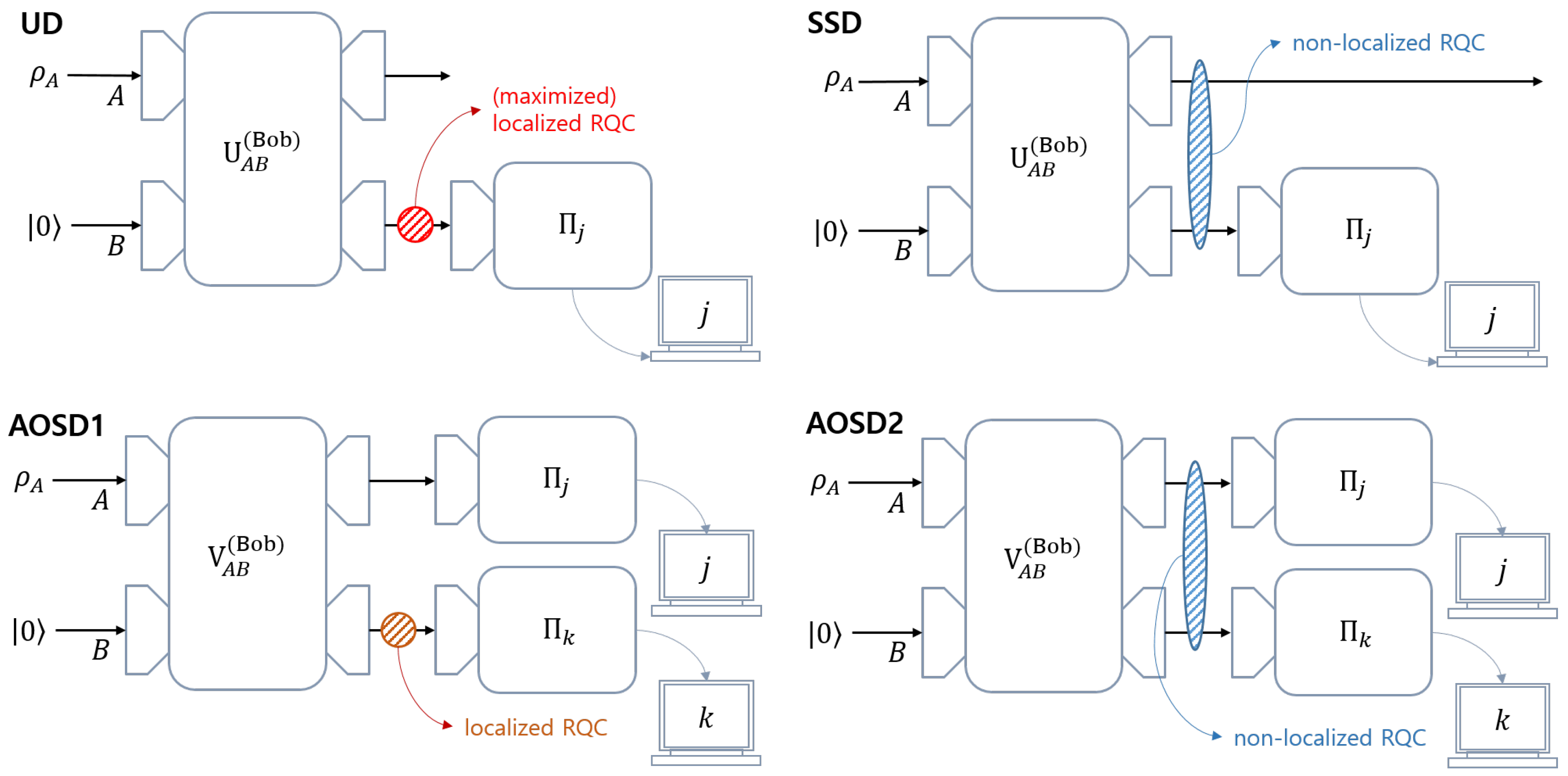
The coherence distribution in UD, SSD, AOSD1, and AOSD2. In UD, the unitary operator localizes the coherence in Alice’s initial ensemble () into Bob’s auxiliary system. In SSD, the unitary operator distributes the coherence in Alice’s initial ensemble into both Alice and Bob’s systems. In AOSD1, the unitary operator localizes the coherence in Alice’s initial ensemble into Bob’s system. In AOSD2, the unitary operator distributes the coherence in Alice’s initial ensemble to both Alice’s and Bob’s systems. This figure shows that the way where coherence distribution occurs depends on the structure of Bob’s measurement.
Figure 7.
The coherence distribution in UD, SSD, AOSD1, and AOSD2. In UD, the unitary operator localizes the coherence in Alice’s initial ensemble () into Bob’s auxiliary system. In SSD, the unitary operator distributes the coherence in Alice’s initial ensemble into both Alice and Bob’s systems. In AOSD1, the unitary operator localizes the coherence in Alice’s initial ensemble into Bob’s system. In AOSD2, the unitary operator distributes the coherence in Alice’s initial ensemble to both Alice’s and Bob’s systems. This figure shows that the way where coherence distribution occurs depends on the structure of Bob’s measurement.

Publisher’s Note: MDPI stays neutral with regard to jurisdictional claims in published maps and institutional affiliations. |
© 2020 by the authors. Licensee MDPI, Basel, Switzerland. This article is an open access article distributed under the terms and conditions of the Creative Commons Attribution (CC BY) license (http://creativecommons.org/licenses/by/4.0/).
Share and Cite
MDPI and ACS Style
Namkung, M.; Kwon, Y. Understanding of Various Type of Unambiguous Discrimination in View of Coherence Distribution. Entropy 2020, 22, 1422. https://doi.org/10.3390/e22121422
AMA Style
Namkung M, Kwon Y. Understanding of Various Type of Unambiguous Discrimination in View of Coherence Distribution. Entropy. 2020; 22(12):1422. https://doi.org/10.3390/e22121422
Chicago/Turabian StyleNamkung, Min, and Younghun Kwon. 2020. "Understanding of Various Type of Unambiguous Discrimination in View of Coherence Distribution" Entropy 22, no. 12: 1422. https://doi.org/10.3390/e22121422
Note that from the first issue of 2016, this journal uses article numbers instead of page numbers. See further details here.