Generalizations of Fano’s Inequality for Conditional Information Measures via Majorization Theory †


Department of Electrical and Computer Engineering, National University of Singapore, 21 Lower Kent Ridge Road, Singapore 119077, Singapore
†
This paper is an extended version of our paper published in the 2018 International Symposium on Information Theory and Its Applications (ISITA’18), Singapore, 28–31 October 2018.
Entropy 2020, 22(3), 288; https://doi.org/10.3390/e22030288
Submission received: 14 November 2019
/
Revised: 15 January 2020
/
Accepted: 27 January 2020
/
Published: 1 March 2020
(This article belongs to the Special Issue Information Measures with Applications)
Abstract
:Fano’s inequality is one of the most elementary, ubiquitous, and important tools in information theory. Using majorization theory, Fano’s inequality is generalized to a broad class of information measures, which contains those of Shannon and Rényi. When specialized to these measures, it recovers and generalizes the classical inequalities. Key to the derivation is the construction of an appropriate conditional distribution inducing a desired marginal distribution on a countably infinite alphabet. The construction is based on the infinite-dimensional version of Birkhoff’s theorem proven by Révész [Acta Math. Hungar. 1962, 3, 188–198], and the constraint of maintaining a desired marginal distribution is similar to coupling in probability theory. Using our Fano-type inequalities for Shannon’s and Rényi’s information measures, we also investigate the asymptotic behavior of the sequence of Shannon’s and Rényi’s equivocations when the error probabilities vanish. This asymptotic behavior provides a novel characterization of the asymptotic equipartition property (AEP) via Fano’s inequality.
Keywords:
Fano’s inequality; countably infinite alphabet; list decoding; general class of conditional information measures; conditional Rényi entropies; α-mutual information; majorization theory; the infinite-dimensional version of Birkhoff’s theorem; the Birkhoff–von Neumann decomposition; asymptotic equipartition property (AEP)1. Introduction
Inequalities relating probabilities to various information measures are fundamental tools for proving various coding theorems in information theory. Fano’s inequality [1] is one such paradigmatic example of an information-theoretic inequality; it elucidates the interplay between the conditional Shannon entropy and the error probability . Denoting by the binary entropy function on with the conventional hypothesis that , Fano’s inequality can be written as
for every , where log stands for the natural logarithm, and the maximization is taken over the jointly distributed pairs of -valued random variables (r.v.’s) X and Y satisfying . An important consequence of Fano’s inequality is that if the error probabilities vanish, so do the normalized equivocations. In other words,
where both and are random vectors in which each component is a -valued r.v. This is the key in proving weak converse results in various communication models (cf. [2,3,4]). Moreover, Fano’s inequality also shows that
where and are -valued r.v.’s for each . This implication is used, for example, to prove that various Shannon’s information measures are continuous in the error metric or the variational distance (cf. [5,6,7]).
1.1. Main Contributions
In this study, we consider general maximization problems that can be specialized to the left-hand side of (1); we generalize Fano’s inequality in the following four ways:
- (i)
- the alphabet of a discrete r.v. X to be estimated is countably infinite,
- (ii)
- the marginal distribution of X is fixed,
- (iii)
- the inequality is established on a general class of conditional information measures, and
- (iv)
- the decoding rule is a list decoding scheme in contrast to a unique decoding scheme.
Specifically, given an -valued r.v. X with a countably infinite alphabet and a -valued r.v. Y with an abstract alphabet , this study considers a generalized conditional information measure defined by
where stands for a version of the conditional probability for each , and stands for the expectation of the real-valued r.v. Z. Here, this function defined on the set of discrete probability distributions on plays the role of an information measure of a discrete probability distribution. When is a countable alphabet, the right-hand side of (4) can be written as
where denotes the probability law of Y, and denotes the conditional probability for each . In this study, we impose some postulates on for technical reasons. Choosing appropriately, we can specialize to the conditional Shannon entropy , Arimoto’s and Hayashi’s conditional Rényi entropies [8,9], and so on. For example, if is given as
then coincides with the conditional Shannon entropy . Denoting by the minimum average probability of list decoding error with a list size L, the principal maximization problem considered in this study can be written as
where the supremum is taken over the pairs satisfying and fixing the -marginal to a given distribution Q. The feasible region of systems will be characterized in this paper to ensure that is well-defined. Under some mild conditions on a given system , especially on the cardinality of , we derive explicit formulas of ; otherwise, we establish tight upper bounds on . As can be thought of as a generalization of the maximization problem stated in (1), we call these results Fano-type inequalities in this paper. These Fano-type inequalities are formulated by the considered information measures of certain (extremal) probability distributions depending only on the system .
In this study, we provide Fano-type inequalities via majorization theory [10]. A proof outline to obtain our Fano-type inequalities is as follows.
- First, we show that a generalized conditional information measure can be bounded from above by with a certain pair in which the conditional distribution of U given V can be thought of as a so-called uniformly dispersive channel [11,12] (see also Section II-A of [13]). We prove this fact via Jensen’s inequality (cf. Proposition A-2 of [14]) and the symmetry of the considered information measures . Moreover, we establish a novel characterization of uniformly dispersive channels via a certain majorization relation; we show that the output distribution of a uniformly dispersive channel is majorized by its transition probability distribution for any fixed input symbol. This majorization relation is used to obtain a sharp upper bound via the Schur-concavity property of the considered information measures .
- Second, we ensure the existence of a joint distribution of which satisfies all constraints in our maximization problems stated in (7) and the conditional distribution is uniformly dispersive. Here, a main technical difficulty is to maintain a marginal distribution of X over a countably infinite alphabet ; see (ii) above. Using a majorization relation for a uniformly dispersive channel, we express a desired marginal distribution by the multiplication of a doubly stochastic matrix and a uniformly dispersive . This characterization of the majorization relation via a doubly stochastic matrix was proven by Hardy–Littleweed–Pólya [15] in the finite-dimensional case, and by Markus [16] in the infinite-dimensional case. From this doubly stochastic matrix, we construct a marginal distribution of Y so that the joint distribution has the desired marginal distribution . The construction of is based on the infinite-dimensional version of Birkhoff’s theorem, which was posed by Birkhoff [17] and was proven by Révész [18] via Kolmogorov’s extension theorem. Although the finite-dimensional version of Birkhoff’s theorem [19] (also known as the Birkhoff–von Neumann decomposition) is well-known, the application of the infinite-dimensional version of Birkhoff’s theorem in information theory appears to be novel; its application aids in dealing with communication systems over countably infinite alphabets.
- Third, we introduce an extremal distribution on a countably infinite alphabet . Showing that is the infimum of a certain class of discrete probability distributions with respect to the majorization relation, our maximization problems can be bounded from above by the considered information measure . Namely, our Fano-type inequality is expressed by a certain information measure of the extremal distribution. When the cardinality of the alphabet of Y is large enough, by constructing a joint distribution achieving equality in our generalized Fano-type inequality, we say that the inequality is sharp.
When the alphabet of Y is finite, we further tighten our Fano-type inequality. To do so, we prove a reduction lemma for the principal maximization problem from an infinite- to a finite-dimensional feasible region. Therefore, when the alphabet of Y is finite, we do not have to employ technical tools in infinite-dimensional majorization theory, e.g., the infinite-dimensional version of Birkhoff’s theorem. This reduction lemma is useful not only to tighten our Fano-type inequality but also to characterize a sufficient condition of the considered information measure in which is finite if and only if is also finite. In fact, Shannon’s and Rényi’s information measures meet this sufficient condition.
We show that our Fano-type inequalities can be specialized to some known generalizations of Fano’s inequality [20,21,22,23] on Shannon’s and Rényi’s information measures. Therefore, one of our technical contributions is a unified proof of Fano’s inequality for conditional information measures via majorization theory. Generalizations of Erokhin’s function [20] from the ordinary mutual information to Sibson’s and Arimoto’s -mutual information [8,24] are also discussed.
Via our generalized Fano-type inequalities, we investigate sufficient conditions on a general source in which vanishing error probabilities implies vanishing equivocations (cf. (2) and (3)). We show that the asymptotic equipartition property (AEP) as defined by Verdú–Han [25] is indeed such a sufficient condition. In other words, if a general source satisfies the AEP and as , then we prove that
where is an arbitrary sequence of list sizes. This is a generalization of (2) and (3) and, to the best of the author’s knowledge, a novel connection between the AEP and Fano’s inequality. We prove this connection by using the splitting technique of a probability distribution; this technique was used to derive limit theorems of Markov processes by Nummelin [26] and Athreya–Ney [27]. Note that there are also many applications of the splitting technique in information theory (cf. [21,28,29,30,31,32]). In addition, we extend Ho–Verdú’s sufficient conditions (See Section V of [21]) and Sason–Verdú’s sufficient conditions (see Theorem 4 of [23]) on a general source in which equivocations vanish if the error probabilities vanish.
1.2. Related Works
1.2.1. Information Theoretic Tools on Countably Infinite Alphabets
As the right-hand side of (1) diverges as M goes to infinity whenever is fixed, the classical Fano inequality is applicable only if X is supported on a finite alphabet (see also Chapter 1 of [33]). In fact, if both and are supported on the same countably infinite alphabet for each , one can construct a somewhat pathological example so that as but for every (cf. Example 2.49 of [4]).
Usually, it is not straightforward to generalize information theoretic tools for systems defined on a finite alphabet to systems defined on a countably infinite alphabet. Ho–Yeung [34] showed that Shannon’s information measures defined on countably infinite alphabets are not continuous with respect to the following distances; the -divergence, the relative entropy, and the variational distance. Continuity issues of Rényi’s information measures defined on countably infinite alphabets were explored by Kovačević–Stanojević–Šenk [35]. In addition, although weak typicality (cf. Chapter 3 of [2] that is also known as the entropy-typical sequences (cf. Problem 2.5 of [6]) is a convenient tool in proving achievability theorems for sources and channels with defined on countably infinite (or even uncountable) alphabets, strong typicality [6] is only amenable in situations with finite alphabets. To ameliorate this issue, Ho–Yeung [36] proposed a notion known as unified typicality that ensures that the desirable properties of weak and strong typicality are retained when one is working with countably infinite alphabets.
Recently, Madiman–Wang–Woo [37] investigated relations between majorization and the strong Sperner property [38] of posets together with applications to the Rényi entropy power inequality for sums of independent and integer-valued r.v.’s, i.e., supported on countably infinite alphabets.
To the best of the author’s knowledge, a generalization of Fano’s inequality to the case when X is supported on a countably infinite alphabet was initiated by Erokhin [20]. Given a discrete probability distribution Q on a countably infinite alphabet , Erokhin established in Equation (11) of [20] an explicit formula of the function:
where the minimization is taken over the pairs of -valued r.v.’s X and Y satisfying and for each , and stands for the mutual information between X and Y. Note that Erokhin’s function is the rate-distortion function with Hamming distortion measures (cf. [39,40]). As the well-known identity implies that
Erokhin’s function can be naturally thought of as a generalization of the classical Fano inequality stated in (1), where stands for the Shannon entropy of X, and the probability distribution of X is given by for each . Kostina–Polyanskiy–Verdú [41] derived a second-order asymptotic expansion of as , where stands for the n-fold product of Q. Their asymptotic expansion is closely related to the second-order asymptotics of the variable-length compression allowing errors; see ([41], Theorem 4).
Ho–Verdú [21] gave an explicit formula of the maximization in the right-hand side of (10); they proved it via the additivity of Shannon’s information measures. Note that Ho–Verdú’s formula (cf. Theorem 1 of [21]) coincides with Erokhin’s formula (cf. Equation (11) of [20]) via the identity stated in (10). In Theorems 2 and 4 of [21], Ho–Verdú also tightened the maximization in the right-hand side of (10) when Y is supported on a proper subalphabet of . Moreover, they provided in Section V of [21] some sufficient conditions on a general source in which vanishing error probabilities (i.e., ) implies vanishing unnormalized or normalized equivocations (i.e., or ).
1.2.2. Fano’s Inequality with List Decoding
Fano’s inequality with list decoding was initiated by Ahlswede–Gács–Körner [42]. By a minor extension of the usual proof (see, e.g., Lemma 3.8 of [6]), one can see that
for every integers and every real number , where the maximization is taken over the pairs of a -valued r.v. X and a -valued r.v. Y satisfying . Note that the right-hand side of (11) coincides with the Shannon entropy of the extremal distribution of type-0 defined by
for each integer . A graphical representation of this extremal distribution is plotted in Figure 1.
Combining (11) and the blowing-up technique (cf. Chapter 5 of [6] or Section 3.6.2 of [43]), Ahlswede–Gács–Körner [42] proved the strong converse property (in Wolfowitz’s sense [44]) of degraded broadcast channels under the maximum error probability criterion. Extending the proof technique in [42] together with the wringing technique, Dueck [45] proved the strong converse property of multiple-access channels under the average error probability criterion. As these proofs rely on a combinatorial lemma (cf. Lemma 5.1 of [6]), they work only when the channel output alphabet is finite; but see recent work by Fong–Tan [46,47] in which such techniques have been extended to Gaussian channels. On the other hand, Kim–Sutivong–Cover [48] investigated a trade-off between the channel coding rate and the state uncertainty reduction of a channel with state information available only at the sender, and derived its trade-off region in the weak converse regime by employing (11).
1.2.3. Fano’s Inequality for Rényi’s Information Measures
So far, many researchers have considered various directions for generalizing Fano’s inequality. An interesting study involves reversing the usual Fano inequality. In this regard, lower bounds on subject to were independently established by Kovalevsky [49], Chu–Cheuh [50], and Tebbe–Dwyer [51] (see also Feder–Merhav’s study [52]). Prasad [53] provided several refinements of the reverse/forward Fano inequalities for Shannon’s information measures.
In [54], Ben-Bassat–Raviv explored several inequalities between the (unconditional) Rényi entropy and the error probability. Generalizations of Fano’s inequality from the conditional Shannon entropy to Arimoto’s conditional Rényi entropy introduced in [8] were recently and independently investigated by Sakai–Iwata [22] and Sason–Verdú [23]. Specifically, Sakai–Iwata [22] provided sharp upper/lower bounds on for fixed with two distinct orders . In other words, they gave explicit formulas of the following minimization and maximization,
respectively. As is a strictly monotone function of the minimum average probability of error if , both functions and can be thought of as reverse and forward Fano inequalities on , respectively (cf. Section V in the arXiv paper [22]). Sason–Verdú [23] also gave generalizations of the forward and reverse Fano’s inequalities on . Moreover, in the forward Fano inequality pertaining to , they generalized in Theorem 8 of [23] the decoding rules from unique decoding to list decoding as follows:
for every and , where the maximization is taken as with (11). Similar to (11), the right-hand side of (15) coincides with the Rényi entropy [55] of the extremal distribution of type-0. Note that the reverse Fano inequality proven in [22,23] does not require that is finite. On the other hand, the forward Fano inequality proven in [22,23] is applicable only when is finite.
1.2.4. Lower Bounds on Mutual Information
Han–Verdú [56] generalized Fano’s inequality on a countably infinite alphabet by investigating lower bounds on the mutual information, i.e.,
via the data processing lemma without additional constraints on the r.v.’s X and Y, where and are independent r.v.’s having marginals as X and Y respectively. Polyanskiy–Verdú [57] showed a lower bound on Sibson’s -mutual information by using the data processing lemma for the Rényi divergence. Recently, Sason [58] generalized Fano’s inequality with list decoding via the strong data processing lemma for the f-divergences.
Liu–Verdú [59] showed that
as , provided that the geometric average probability of error, which is a weaker and a stronger criteria than the maximum and the average error criteria, respectively, satisfies
for sufficiently large n, where is a r.v. uniformly distributed on the codeword set , is a r.v. induced by the n-fold product of a discrete memoryless channel with the input , is a positive integer denoting the message size, is a collection of disjoint subsets playing the role of decoding regions, and is a tolerated probability of error. This is a second-order asymptotic estimate on the mutual information, and is derived by using the Donsker–Varadhan lemma (cf. Equation (3.4.67) of [43]) and the so-called pumping-up argument.
1.3. Paper Organization
The rest of this paper is organized as follows. Section 2 introduces basic notations and definitions to understand our generalized conditional information measure and the principal maximization problem . Section 3 presents the main results: our Fano-type inequalities. Section 4 specializes our Fano-type inequalities to Shannon’s and Rényi’s information measures, and discusses generalizations of Erokhin’s function from the ordinary mutual information to Sibson’s and Arimoto’s -mutual information. Section 5 investigates several conditions on a general source in which the vanishing error probabilities implies the vanishing equivocations; a novel characterization of the AEP via Fano’s inequality is also presented. Section 6 proves our Fano-type inequalities stated in Section 3, and contains most technical contributions in this study. Section 7 proves the asymptotic behaviors stated in Section 5. Finally, Section 8 concludes this study with some remarks.
2. Preliminaries
2.1. A General Class of Conditional Information Measures
This subsection introduces some notions in majorization theory [10] and a rigorous definition of generalized conditional information measure defined in (4). Let be a countably infinite alphabet. A discrete probability distribution P on is a map satisfying . In this paper, motivated to consider the joint probability distributions on , it is called an -marginal. Given an -marginal P, a decreasing rearrangement of P is denoted by , i.e., it fulfills
The following definition gives us the notion of majorization for -marginals.
Definition 1
(Majorization [10]). An -marginal P is said to majorize another -marginal Q if
for every . This relation is denoted by or .
Let be the set of -marginals. The following definitions are important postulates on a function playing the role of an information measure of an -marginal.
Definition 2.
A function is said to be symmetric if it is invariant for any permutation of probability masses, i.e., for every .
Definition 3.
A function is said to be lower semicontinuous if for any , it holds that for every pointwise convergent sequence , where the pointwise convergence means that as for every .
Definition 4.
A function is said to be convex if with for every and .
Definition 5.
A function is said to be quasiconvex if the sublevel set is convex for every and .
Definition 6.
A function is said to be Schur-convex if implies that .
In Definitions 4–6, each term or its suffix convex is replaced by concave if fulfills the condition. In Definition 3, note that the pointwise convergence of -marginals is equivalent to the convergence in the variational distance topology (see, e.g., Lemma 3.1 of [60] or Section III-D of [61]).
Let X be an -valued r.v. and Y a -valued r.v., where is an abstract alphabet. Unless stated otherwise, assume that the measurable space of with a certain -algebra is standard Borel, where a measurable space is said to be standard Borel if its -algebra is the Borel -algebra generated by a Polish topology on the space. Assuming that is a symmetric, concave, and lower semicontinuous function, the generalized conditional information measure is defined by (4). The postulates on we have imposed here are useful for technical reasons to employ majorization theory; see the following lemma.
Proposition 1.
Every symmetric and quasiconvex function is Schur-convex.
Proof of Proposition 1.
To employ the Schur-concavity property in the sequel, Proposition 1 suggests assuming that is symmetric and quasiconcave. In addition, to apply Jensen’s inequality on the function , it suffices to assume that is concave and lower semicontinuous, because the domain forms a closed convex bounded set in the variational distance topology (cf. Proposition A-2 of [14]). Motivated by these properties, we impose the three postulates (corresponding to Definitions 2–4) on in this study.
2.2. Minimum Average Probability of List Decoding Error
Consider a certain communication model for which a -valued r.v. Y plays the role of the side-information of an -valued r.v. X. A list decoding scheme with a list size is a decoding scheme producing L candidates for realizations of X when we observe a realization of Y. The minimum average error probability under list decoding is defined by
where the minimization is taken over all set-valued functions with the decoding range
and stands for the cardinality of a set. If is an infinite set, then we assume that as usual. If , then (21) coincides with the average error probability of the maximum a posteriori (MAP) decoding scheme. For the sake of brevity, we write
It is clear that
for any list decoder and any tolerated probability of error . Therefore, it suffices to consider the constraint rather than in our subsequent analyses.
The following proposition is an elementary formula of as in the MAP decoding.
Proposition 2.
It holds that
Proof of Proposition 2.
See Appendix A. □
Remark 1.
It follows from Proposition 2 that defined in (4) can be specialized to with
The following proposition characterizes the feasible region of systems considered in our principal maximization problem stated in (7).
Proposition 3.
If , then
Moreover, both inequalities are sharp in the sense that there exist pairs of r.v.’s X and Y achieving the equalities while respecting the constraint .
Proof of Proposition 3.
See Appendix B. □
The minimum average error probability for list decoding concerning without any side-information is denoted by
Then, the second inequality in (27) is obvious, and it is similar to the property that conditioning reduces uncertainty (cf. [2], Theorem 2.8.1). Proposition 3 ensures that when we have to consider the constraints and , it suffices to consider a system satisfying
3. Main Results: Fano-Type Inequalities
Let be a system satisfying (29), and a symmetric, concave, and lower semicontinuous function. The main aim of this study is to find an explicit formula or a tight upper bound on defined in (7). Now, define the extremal distribution of type-1 by the following -marginal,
for each , the weight is defined by
for each , the weight is defined by
for each , the integer J is chosen so that
and is chosen so that
A graphical representation of is shown in Figure 2. Under some mild conditions, the following theorem gives an explicit formula of .
Theorem 1.
Suppose that and the cardinality of is at least countably infinite. Then, it holds that
Proof of Theorem 1.
See Section 6.1. □
The Fano-type inequality stated in (35) of Theorem 1 is formulated by the extremal distribution defined in (30). The following proposition summarizes basic properties of .
Proposition 4.
The extremal distribution of type-1 defined in (30) satisfies the following,
- the probability masses are nonincreasing in , i.e.,
- the sum of first L probability masses of is equal to , i.e.,consequently, it holds that
- the first probability masses are equal to that of , i.e.,
- the probability masses for are equal to , i.e.,
- the probability masses for are equal to , i.e.,
- the probability masses for are equal to that of , i.e.,and
- it holds that majorizes Q.
Proof of Proposition 4.
See Appendix C. □
Although positive tolerated probabilities of error (i.e., ) are highly interesting in most of the lossless communication systems, the scenario in which the error events with positive probabilities are not allowed (i.e., ) is also important to deal with the error-free communication systems. The following theorem is an error-free version of Theorem 1.
Theorem 2.
Suppose that and is at least countably infinite. Then, it holds that
with equality if is finite or . Moreover, if the cardinality of is at least the cardinality of the continuum , then there exists a σ-algebra on satisfying (43) with equality.
Proof of Theorem 2.
See Section 6.2. □
Remark 2.
Note that holds under the unique decoding rule (i.e., ); that is, we see from Theorem 2 that (43) holds with equality if . The inequality occurs only if a non-unique decoding rule (i.e., ) is considered. In Theorem 2, the existence of a σ-algebra on an uncountably infinite alphabet in which (43) holds with equality is due to Révész’s generalization of the Birkhoff–von Neumann decomposition via Kolmogorov’s extension theorem; see Section 6.1 and Section 6.2 for technical details.
Consider the case where is a finite alphabet. Define the extremal distribution of type-2 as the following -marginal,
for each , where the three quantities , , and J are defined in (31), (32), and (33), respectively, and is chosen so that
Moreover, define the integer D by
where stands for the binomial coefficient for two integers . A graphical representation of is illustrated in Figure 3. When is finite, the Fano-type inequality stated in Theorems 1 and 2 can be tightened as follows:
Theorem 3.
Suppose that is finite. Then, it holds that
with equality if or .
Proof of Theorem 3.
See Section 6.3. □
Similar to Theorems 1 and 2, the Fano-type inequality stated in (47) of Theorem 3 is formulated by the extremal distribution defined in (44). The difference between and is only the difference between and defined in (34) and (45), respectively.
Remark 3.
In contrast to Theorems 1 and 2, Theorem 3 holds in both cases: and . By Lemma 5 stated in Section 6.1, it can be verified that majorizes , and it follows from Proposition 1 that
Namely, the Fano-type inequalities stated in Theorems 1 and 2 also holds for finite . In other words, it holds that
for every nonempty alphabet , provided that satisfies (29). As if (see (46)), another benefit of Theorem 3 is that the Fano-type inequality is always sharp under a unique decoding rule (i.e., ).
So far, it is assumed that the probability law of the -valued r.v. X is fixed to a given -marginal Q. When we assume that X is supported on a finite subalphabet of , we can loosen and simplify our Fano-type inequalities by removing the constraint that . Let L and M be two integers satisfying , a real number satisfying , and a nonempty alphabet. Consider the following maximization,
where the maximization is taken over the pairs of r.v.’s satisfying (i) X is -valued, (ii) Y is -valued, and (iii) .
Theorem 4.
Proof of Theorem 4.
See Section 6.4. □
Remark 4.
Although Theorems 1–3 depend on the cardinality of , the Fano-type inequality stated in Theorem 4 does not depend on it whenever is nonempty.
4. Special Cases: Fano-Type Inequalities on Shannon’s and Rényi’s Information Measures
In this section, we specialize our Fano-type inequalities stated in Theorems 1–4 from general conditional information measures to Shannon’s and Rényi’s information measures. We then recover several known results such as those in [1,20,21,22,23] along the way.
4.1. On Shannon’s Information Measures
The conditional Shannon entropy [62] of an -valued r.v. X given a -valued r.v. Y is defined by
where the (unconditional) Shannon entropy of an -marginal P is defined by
Remark 5.
The following proposition is a well-known property of Shannon’s information measures.
Proposition 5
(Topsøe [60]). The Shannon entropy is symmetric, concave, and lower semicontinuous.
Namely, the conditional Shannon entropy is a special case of with . Therefore, defining the quantity
we readily observe the following corollary.
Corollary 1.
Suppose that and the cardinality of is at least countably infinite. Then, it holds that
Proof of Corollary 1.
Corollary 1 is a direct consequence of Theorem 1 and Proposition 5. □
Remark 6.
Applying Theorem 2 instead of Theorem 1, an error-free version (i.e., ) of Corollary 1 can be considered.
Remark 7.
Note that Corollary 1 coincides with Theorem 1 of [21] if and . Moreover, we observe from (10) and Corollary 1 that
for every -marginal Q and every tolerated probability of error , where Erokhin’s function is defined in (9). See Section 4.3 for details of generalizing of Erokhin’s function. Kostina–Polyanskiy–Verdú showed in Theorem 4 and Remark 3 of [41] that
where is defined by
and stands for the inverse of the Gaussian cumulative distribution function
If is finite, then a tighter version of the Fano-type inequality than Corollary 1 can be obtained as follows:
Corollary 2.
Suppose that is finite. Then, it holds that
with equality if or .
Proof of Corollary 2.
Corollary 2 is a direct consequence of Theorem 3 and Proposition 5. □
Remark 8.
Corollary 3.
It holds that
Proof of Corollary 3.
(Corollary 3 is a direct consequence of Theorem 4 and Proposition 5. □
Remark 9.
Indeed, Corollary 3 states the classical Fano inequality with list decoding; see (11).
4.2. On Rényi’s Information Measures
Although the choices of Shannon’s information measures are unique based on a set of axioms (see, e.g., Theorem 3.6 of [6] and Chapter 3 of [4]), there are several different definitions of conditional Rényi entropies (cf. [65,66,67]). Among them, this study focuses on Arimoto’s and Hayashi’s conditional Rényi entropies [8,9]. Arimoto’s conditional Rényi entropy of X given Y is defined by
for each order , where the -norm of an -marginal P is defined by
Here, note that the (unconditional) Rényi entropy [55] of an -marginal P can be defined by
i.e., it is a monotone function of the -norm. Basic properties of the -norm can be found in the following proposition.
Proposition 6.
The -norm is symmetric and lower semicontinuous. Moreover, it is concave (resp. convex) if (resp. if ).
Proof of Proposition 6.
The symmetry is obvious. The lower semicontinuity was proven by Kovačević–Stanojević–Šenk in Theorem 5 of [35]. The concavity (resp. convexity) property can be verified by the reverse (resp. forward) Minkowski inequality. □
Proposition 6 implies that is a monotone function of with , i.e.,
On the other hand, Hayashi’s conditional Rényi entropy of X given Y is defined by
for each order . It is easy to see that also admits the same properties as those stated in Proposition 6. Therefore, Hayashi’s conditional Rényi entropy is also a monotone function of with , i.e.,
It can be verified by Jensen’s inequality (see, e.g., Proposition 1 of [66]) that
Similar to (7), we now define
for each and each . Then, we can establish the Fano-type inequality on Rényi’s information measures as follows.
Corollary 4.
Suppose that and the cardinality of is at least countably infinite. For every and , it holds that
Proof of Corollary 4.
Remark 10.
Applying Theorem 2 instead of Theorem 1, an error-free version (i.e., ) of Corollary 4 can be considered.
Remark 11.
Although Hayashi’s conditional Rényi entropy is smaller than Arimoto’s one in general (see (70)), Corollary 4 implies that the maximization problem results in the same Rényi entropy for each .
When is finite, a tighter Fano-type inequality than Corollary 4 can be obtained as follows.
Corollary 5.
Suppose that is finite. For any and , it holds that
with equality if or .
Proof of Corollary 5.
The proof is the same as the proof of Corollary 4 by replacing Theorem 1 by Theorem 3. □
Corollary 6.
For every and , it holds that
Proof of Corollary 6.
The proof is the same as the proof of Corollary 4 by replacing Theorem 1 by Theorem 4. □
Remark 12.
Remark 13.
It follows by l’Hôpital’s rule that
Therefore, our Fano-type inequalities stated in Corollaries 1–6 satisfy the continuity of Shannon’s and Rényi’s information measures with respect to the order .
4.3. Generalization of Erokhin’s Function to α-Mutual Information
Erokhin’s function defined in (9) can be generalized to the -mutual information (cf. [68]) as follows: Let X be an -valued r.v. and Y a -valued r.v. Sibson’s -mutual information [24] (see also Equation (32) of [68], Equation (13) of [69], and Definition 7 of [70]) is defined by
for each , where (resp. ) denotes the probability measure on (resp. ) induced by the pair of r.v.’s (resp. the r.v. X), the infimum is taken over the probability measures on , and the Rényi divergence [55] between two probability measures and on is defined by
for each . Note that Sibson’s -mutual information coincides with the ordinary mutual information when , i.e., it holds that . Similar to (7) and (9), given a system satisfying (29), define
where the infimum is taken over the pairs of r.v.’s X and Y in which (i) X is -valued, (ii) Y is -valued, (iii) , and (iv) . By convention, we denote by
It is clear that this definition can be specialized to Erokhin’s function defined in (9); in other words, it holds that
see Remark 7.
Corollary 7
(When ). Suppose that and the cardinality of is at least countably infinite. Then, it holds that
Proof of Corollary 7.
Corollary 8
(Sibson, when ). Suppose that and is countably infinite. For every , it holds that
where stands for the s-tilted distribution of Q with real parameter , i.e.,
for each , and , , , and are defined as in (31), (32), (33), and (34), respectively, by replacing the -marginal Q by the s-tilted distribution .
Proof of Corollary 8.
As Sibson’s identity [24] (see also [69], Equation (12)) states that
where stands for the probability distribution on given as
for each , we observe that
for every , provided that is countable. On the other hand, it follows from ([8] Equation (13)) that
for every , provided that is countable. Combining (92) and (93), we have the first equality in (88). Finally, the second equality in (88) follows from Corollary 4 after some algebra. This completes the proof of Corollary 8. □
In contrast to (82), Arimoto defined the -mutual information ([8], Equation (15)) by
for every . Similar to (84), one can define
and a counterpart of Corollary 8 can be stated as follows.
Corollary 9
(Arimoto, when ). Suppose that and the cardinality of is at least countably infinite. For every , it holds that
Proof of Corollary 9.
When is finite, then the inequalities stated in Corollaries 7–9 can be tightened by Theorem 3 as in Corollaries 2 and 5. We omit to explicitly state these tightened inequalities in this paper.
5. Asymptotic Behaviors on Equivocations
In information theory, the equivocation or the remaining uncertainty of an r.v. X relative to a correlated r.v. Y has an important role in establishing fundamental limits of the optimal transmission ratio and/or rate in several communication models. Shannon’s equivocation is a well-known measure in the formulation of the notion of perfect secrecy of symmetric-key encryption in information-theoretic cryptography [71]. Iwamoto–Shikata [66] considered the extension of such a secrecy criterion by generalizing Shannon’s equivocation to Rényi’s equivocation by showing various desired properties of the latter. Recently, Hayashi–Tan [72] and Tan–Hayashi [73] studied the asymptotics of Shannon’s and Rényi’s equivocations when the side-information about the source is given via a various class of random hash functions with a fixed rate.
In this section, we assume that certain error probabilities vanish and we then establish asymptotic behaviors on Shannon’s, or sometimes on Rényi’s, equivocations via the Fano-type inequalities stated in Section 4.
5.1. Fano’s Inequality Meets the AEP
We consider a general form of the asymptotic equipartition property (AEP) as follows.
Definition 7
In the literature, the r.v. is commonly represented as a random vector . The formulation without reference to random vectors means that is a general source in the sense of Page 100 of [33].
Let be a sequence of positive integers, a sequence of nonempty alphabets, and a sequence of pairs of r.v.’s, where (resp. ) is -valued (resp. -valued) for each . As
for any sequence of list decoders , it suffices to assume that as in our analysis. The following theorem is a novel characterization of the AEP via Fano’s inequality.
Theorem 5.
Suppose that a general source satisfies the AEP, and as . Then, it holds that
where for . Consequently, it holds that
Proof of Theorem 5.
See Section 7.1. □
The following three examples are particularizations of Theorem 5.
Example 1.
Let be an i.i.d. source on a countably infinite alphabet with finite Shannon entropy . Suppose that and for each . Then, Theorem 5 states that
This result is commonly referred to as the weak converse property of the source in the unique decoding setting.
Example 2.
Let be a source as described in Example 1. Even if the list decoding setting, Theorem 5 states that
similarly to Example 1. This is a key observation in Ahlswede–Gács–Körner’s proof of the strong converse property of degraded broadcast channels; see Chapter 5 of [42] (see also Section 3.6.2 of [43] and Lemma 1 of [48]).
Example 3.
Consider the Poisson source with growing mean as , i.e.,
It is known that
and the Poisson source satisfies the AEP (see [25]). Therefore, it follows from Theorem 5 that
The following example shows a general source that satisfies neither the AEP nor (99).
Example 4.
Let be an integer, a positive real, and a sequence of reals satisfying and for each . As is continuous on and as , one can find a sequence of reals satisfying for each and
Consider a general source whose component distributions are given by
for each . Suppose that for each . After some algebra, we have
for each . Therefore, we observe that
holds, but
does not hold. In fact, it holds that as and
Consequently, we also see that does not satisfy the AEP.
Example 4 implies that the AEP has an important role in Theorem 5.
5.2. Vanishing Unnormalized Rényi’s Equivocations
Let X be an -valued r.v. satisfying , a sequence of positive integers, a sequence of nonempty alphabets, and a sequence of -valued r.v.’s. The following theorem provides four conditions on a general source such that vanishing error probabilities implies vanishing unnormalized Shannon’s and Rényi’s equivocations.
Theorem 6.
Let be an order. Suppose that any one of the following four conditions hold,
- (a)
- the order α is strictly larger than 1, i.e., ,
- (b)
- the sequence satisfies the AEP and as ,
- (c)
- there exists an such that majorizes for every ,
- (d)
- the sequence converges in distribution to X and as .
Then, it holds that for each ,
Proof of Theorem 6.
See Section 7.2. □
In contrast to Condition (b) of Theorem 6, Conditions (a), (c), and (d) of Theorem 6 do not require the AEP to hold. Interestingly, Condition (a) of Theorem 6 states that (113) holds for every and without any other conditions on the general source .
5.3. Under the Symbol-Wise Error Criterion
Let be a sequence of positive integers, a sequence of nonempty alphabets, and a sequence of -valued r.v.’s satisfying for every . In this subsection, we focus on the minimum arithmetic-mean probability of symbol-wise list decoding error defined as
where and . Now, let X be an -valued r.v. satisfying . Under this symbol-wise error criterion, the following theorem holds.
Theorem 7.
Suppose that majorizes for sufficiently large n. Then, it holds that
Proof of Theorem 7.
See Section 7.3. □
It is known that the classical Fano inequality stated in (1) can be extended from the average error criterion to the symbol-wise error criterion (see Corollary 3.8 of [6]), where
stands for the Hamming distance between two strings and . In fact, Theorem 7 states that
provided that majorizes for sufficiently large n.
However, in the list decoding setting, we observe that does not imply in general. A counterexample can be readily constructed.
Example 5.
Let be uniformly distributed Bernoulli r.v.’s, and arbitrary r.v.’s. Suppose that if , for each , and for each . Then, we observe that
for every , but
for every .
6. Proofs of Fano-Type Inequalities
In this section, we prove Theorems 1–4 via majorization theory [10].
6.1. Proof of Theorem 1
We shall relax the feasible regions of the supremum in (7) via some lemmas, i.e., our preliminary results. Define a notion of symmetry for the conditional distribution as follows.
Definition 8.
A jointly distributed pair is said to be connected uniform-dispersively if is almost surely constant.
Remark 15.
The term introduced in Definition 8 is inspired by uniformly dispersive channels named by Massey (see Page 77 of [12]). In fact, if is countable and X (resp. Y) denotes the output (resp. input) of a channel , then the channel can be thought of as a uniformly dispersive channel, provided that is connected uniform-dispersively. Initially, Fano said such channels to be uniform from the input; see Page 127 of [11]. Refer to Section II-A of [13] for several symmetry notions of channels.
Although an almost surely constant implies the independence , note also that an almost surely constant does not imply the independence. We now give the following lemma.
Lemma 1.
If a jointly distributed pair is connected uniform-dispersively, then majorizes a.s.
Proof of Lemma 1.
Let k be a positive integer. Choose a collection of k distinct elements in so that
for every . As
and
for each , we observe that
If is connected uniform-dispersively (see Definition 8), then (123) implies that
which is indeed the majorization relation stated Definition 1, completing the proof of Lemma 1. □
Remark 16.
Lemma 1 is can be thought of as a novel characterization of uniformly dispersive channels via the majorization relation; see Remark 15. More precisely, given an input distribution P on and a uniformly dispersive channel with countable output alphabet , it holds that majorizes the output distribution for every , where is given by
for each .
Definition 9.
Let be a collection of jointly distributed pairs of an -valued r.v. and a -valued r.v. We say that has balanced conditional distributions if implies that there exists satisfying
for every .
For such a collection , the following lemma holds.
Lemma 2.
Suppose that has balanced conditional distributions. For any , there exists a pair connected uniform-dispersively such that
Proof of Lemma 2.
For any , it holds that
where
This completes the proof of Lemma 2. □
For a system satisfying (29), we now define a collection of pairs of r.v.’s as follows,
Note that this is the feasible region of the supremum in (7). The main idea of proving Theorem 1 is to apply Lemma 2 for this collection. The collection does not, however, have balanced conditional distributions in general. More specifically, there exists a measurable space such that does not have balanced conditional distributions even if is standard Borel. Fortunately, the following lemma can avoid this issue by blowing-up the collection via the infinite-dimensional version of Birkhoff’s theorem [18].
Lemma 3.
If the cardinality of is at least the cardinality of the continuum , then there exists a σ-algebra on such that the collection has balanced conditional distributions.
Proof of Lemma 3.
First, we shall choose an appropriate alphabet so that its cardinality is the cardinality of the continuum. Denote by the set of permutation matrices, where an permutation matrix is a real matrix satisfying either or for each , and
For an permutation matrix , define the permutation on by
It is known that there is a one-to-one correspondence between the permutation matrices and the bijections ; and thus, the cardinality of is the cardinality of the continuum. Therefore, in this proof, we may assume without loss of generality that .
Second, we shall construct an appropriate -algebra on via the infinite-dimensional version of Birkhoff’s theorem (cf. Theorem 2 of [18]) for doubly stochastic matrices, where an doubly stochastic matrix is a real matrix satisfying for each , and
Similar to , denote by the set of permutation matrices in which the entry in the ith row and the jth column is 1, where note that . Then, the following lemma holds.
Lemma 4
(infinite-dimensional version of Birkhoff’s theorem; cf. Theorem 2 of [18]). There exists a σ-algebra Γ on such that (i) for every and (ii) for any doubly stochastic matrix , there exists a probability measure μ on such that for every .
Remark 17.
This is a probabilistic description of an doubly stochastic matrix via a probability measure on the permutation matrices. The existence of the probability measure is due to Kolmogorov’s extension theorem. We employ this -algebra on in the proof.
Thirdly, we shall show that under this measurable space , the collection has balanced conditional distributions defined in (126). In other words, for a given pair , it suffices to construct another pair of r.v.’s satisfying (126) and . At first, construct its conditional distribution by
for each , where stands for the conditional expectation of a real-valued r.v. Z given the sub--algebra generated by a r.v. W, and is given as in (132). As is -measurable for each , it is clear that
for every . Thus, we readily see that (126) holds, and is connected uniform-dispersively. Thus, by (123) and the hypothesis that , we see that majorizes Q a.s. Therefore, it follows from the well-known characterization of the majorization relation via doubly stochastic matrices (see Lemma 3.1 of [16] or Page 25 of [10]) that one can find an doubly stochastic matrix satisfying
for every . By Lemma 4, we can construct an induced probability measure so that for each . Now, the pair of and can define the probability law of . To ensure that belongs to , it remains to verity that and .
As is a permutation defined in (132), we have
where
- (a) and (c) follow from Proposition 2, and
- and (b) follows from (136).
Therefore, we see that is equivalent to . Furthermore, we observe that
for every , where
- (a) follows from (137),
- (b) follows by the identity ,
- (c) follows from the fact that is connected uniform-dispersively,
- (d) follows from (136),
- (e) follows by the definition of ,
- (f) follows by the Fubini–Tonelli theorem, and
- (f) follows from the fact that the inverse of a permutation matrix is its transpose.
Therefore, we have , and the assertion of Lemma 3 is proved in the case where the cardinality of is the cardinality of the continuum.
Finally, even if the cardinality of is larger than the cardinality of continuum, the assertion of Lemma 3 can be immediately proved by considering the trace of the space on (cf. [74], p. 23). This completes the proof of Lemma 3. □
Finally, we show that the Fano-type distribution of type-1 defined in (30) is the infimum of a certain class of -marginals with respect to the majorization relation ≺.
Lemma 5.
Suppose that the system satisfies the right-hand inequality in (29). For every -marginal R in which R majorizes Q and , it holds that R majorizes as well.
Proof of Lemma 5.
We first give an elementary fact of the weak majorization on the finite-dimensional real vectors.
Lemma 6.
Let and be n-dimensional real vectors satisfying and , respectively. Consider an integer satisfying for every . If
then it holds that
Proof of Lemma 6.
See Appendix E. □
Since (see Proposition 4), it suffices to prove that
for every .
As for each (see Proposition 4), it follows by the majorization relation that (143) holds for each . Moreover, as (see Proposition 4), it follows from (28) and the hypothesis that
In addition, as (143) holds for each and for each (see Proposition 4), it follows from Lemma 6 and (144) that (143) also holds for each .
Now, suppose that . Then, it follows that
for each (see Proposition 4). Thus, Inequality (143) holds for every ; therefore, we have that R majorizes , provided that .
Finally, suppose that . Since for each (see Proposition 4), it follows by the majorization relation that (143) holds for every . Moreover, since (143) holds for every and every , we observe that
Finally, as (143) holds for and for (see Proposition 4), it follows by Lemma 6 and (146) that (143) holds for every . Therefore, Inequality (143) holds for every , completing the proof of Lemma 5. □
Using the above lemmas, we can prove Theorem 1 as follows.
Proof of Theorem 1.
Let . For the sake of brevity, we write
in the proof. Let be a -algebra on , an alphabet in which its cardinality is the cardinality of the continuum, and a -algebra on so that has balanced conditional distributions (see Lemma 3). Now, we define the collection
where the -algebra on is given by the smallest -algebra containing and . It is clear that , and has balanced conditional distributions as well (see the last paragraph in the proof of Lemma 3). Then, we have
where
- (a) follows by the definition of stated in (129),
- (b) follows by the inclusion ,
- (c) follows from Lemma 2 and the fact that has balanced conditional distributions,
- (d) follows by the symmetry of both and ,
- (e) follows from Lemma 1, and
- (f) follows from Proposition 1 and Lemma 5.
Inequalities (149) are indeed the Fano-type inequality stated in (35) of Theorem 1. If , then it can be verified by the definition of stated in (30) that (see also Proposition 4). In such a case, the supremum in (7) can be achieved by a pair satisfying and .
Finally, we shall construct a jointly distributed pair satisfying
For the sake of brevity, suppose that is the index set of the set of permutation matrices on . Namely, denote by a permutation matrix for each index . By the definition of stated in (30) (see also Proposition 4), we observe that
and
Noting that if (see (34)), Equations (153) and (154) are indeed a majorization relation between two finite-dimensional real vectors; and thus, it follows from the Hardy–Littlewood–Pólya theorem (see Theorem 8 of [15] or Theorem 2.B.2 [10]) that there exists a doubly stochastic matrix satisfying
for each . Moreover, it follows from the finite dimensional version of Birkhoff’s theorem [19] (see also Theorems 2.A.2 and 2.C.2 of [10]) that for such a doubly stochastic matrix , there exists a probability vector satisfying
for every , where a nonnegative vector is called a probability vector if the sum of the elements is unity. Using them, we construct a pair via the following distributions,
where the permutation on is defined by
for each . Then, it follows from (155) and (156) that (152) holds. Moreover, it is easy to see that for every . Thus, we observe that (150) and (151) hold as well. This implies together with (149) that the constructed pair achieves the supremum in (7), completes the proof of Theorem 1. □
6.2. Proof of Theorem 2
Even if , the inequalities in (149) hold as well; that is, the Fano-type inequality stated in (43) of Theorem 2 holds. In this proof, we shall verify the equality conditions of (43).
If is finite, then it follows by the definition of stated in (34) that . Thus, the same construction of a jointly distributed pair as the last paragraph of Section 6.1 proves that (43) holds with equality if is finite.
Consider the case where is infinite and . Since , we readily see that , , and . Suppose that
We then construct a pair via the following distributions,
We readily see that for every ; therefore, we have that (150)–(152) hold. This implies that the constructed pair achieves the supremum in (7).
Finally, suppose that the cardinality of is at least the cardinality of the continuum. Assume without loss of generality that is the set of permutation matrices. Consider the measurable space given in the infinite-dimensional version of Birkhoff’s theorem (see Lemma 4). In addition, consider a jointly distributed pair satisfying a.s. Then, it is easy to see that (150) and (151) hold for any induced probability measure on . Similar to the construction of the probability measure on below (137), we can find an induced probability measure satisfying (152). Therefore, it follows from (43) that this pair achieves the supremum in (7). This completes the proof of Theorem 2.
6.3. Proof of Theorem 3
To prove Theorem 3, we need some more preliminary results. Throughout this subsection, assume that the alphabet is finite and nonempty. In this case, given a pair , one can define
provided that .
For a subset , define
Note that the difference between and is the restriction of the decoding range , and the inequality is trivial from these definitions stated in (21) and (164), respectively. The following propositions are easy consequences of the proofs of Propositions 2 and 3, and so we omit those proofs in this paper.
Proposition 7.
It holds that
Proposition 8.
Let be a bijection satisfying if . It holds that
For a finite subset , denote by the set of permutation matrices in which both rows and columns are indexed by the elements in . The main idea of proving Theorem 3 is the following lemma.
Lemma 7.
For any -valued r.v. , there exist a subset and an -valued r.v. such that
Proof of Lemma 7.
Suppose without loss of generality that
for some positive integer N. By the definition of cardinality, one can find a subset satisfying (i) , and (ii) for each and , there exists satisfying
For each , define the permutation by
as in (132) and (159). It is clear that for each , there exists at least one such that
for every satisfying , which implies that the permutation plays the role of a decreasing rearrangement of on . To denote such a correspondence between and , one can choose an injection appropriately. In other words, one can find an injection so that
for every and satisfying . We now construct an -valued r.v. as follows: The conditional distribution is given by
where stands for the composition of two bijections and . The induced probability distribution of V is given by . Suppose that the independence holds. As
it remains to determine the induced probability distribution of W, and we defer to determine it until the last paragraph of this proof. A direct calculation shows
where
- (a) follows by the independence and , and
- (b) follows by (177) and defining so thatfor each and .
Now, we readily see from (179) that (171) holds for any induced probability distribution of W. Therefore, to complete the proof, it suffices to show that satisfies (169) and (170) with an arbitrary choice of , and satisfies (168) with an appropriate choice of .
Firstly, we shall prove (169). For each , denote by the set satisfying
for every and , i.e., it stands for the set of first L elements in under the permutation rule . Then, we have
where
Therefore, we obtain (169).
Secondly, we shall prove (170). We get
where
- (a) follows by the symmetry of and (177),
- (b) follows by ,
- (c) follows by Jensen’s inequality, and
- (d) follows by the independence .
Therefore, we obtain (170).
Finally, we shall prove that there exists an induced probability distribution satisfying (168). If we denote by the identity matrix, then it follows from (180) that
for every . It follows from (179) that
Now, denote by and two bijections satisfying and , respectively, provided that . That is, the bijection and play roles of decreasing rearrangements of and , respectively, on . Using those bijections, one can rewrite (185) as
In the same way as (123), it can be verified from (180) by induction that
for each . Equations (186) and (187) are indeed a majorization relation between two finite-dimensional real vectors, because plays a role of a decreasing rearrangement of on . Combining (184) and this majorization relation, it follows from the Hardy–Littlewood–Pólya theorem derived in Theorem 8 of [15] (see also Theorem 2.B.2 of [10]) and the finite-dimensional version of Birkhoff’s theorem [19] (see also Theorem 2.A.2 of [10]) that there exists an induced probability distribution satisfying , i.e., Equation (168) holds, as in (153)–(158). This completes the proof of Lemma 7. □
Remark 18.
Lemma 7 can restrict the feasible region of the supremum in (7) from a countably infinite alphabet to a finite alphabet in the sense of (171). Specifically, if is finite, it suffices to vary at most probability masses for each . Lemma 7 is useful not only to prove Theorem 3 but also to prove Proposition 9 of Section 8.1 (see Appendix D for the proof).
As with (129), for a subset , we define
provided that is finite. It is clear that (188) coincides with (129) if , i.e., it holds that
Note from Lemma 7 that for each system satisfying (29), there exists a subset such that and is nonempty, provided that is finite.
Another important idea of proving Theorem 3 is to apply Lemma 2 for this collection of r.v.’s. The correction does not, however, have balanced conditional distributions of (126) in general, as with (129). Fortunately, similar to Lemma 3, the following lemma can avoid this issue by blowing-up the collection via the finite-dimensional version of Birkhoff’s theorem [19].
Lemma 8.
Suppose that is finite and is nonempty. If , then the collection has balanced conditional distributions.
Proof of Lemma 8.
Lemma 8 can be proven in a similar fashion to the proof of Lemma 3. As this proof is slightly long as with Lemma 3, we only give a sketch of the proof as follows.
As , we may assume without loss of generality that . For the sake of brevity, we write
in this proof. For a pair , construct another -valued r.v. , as in (135), so that for every . By such a construction of (135), the condition stated in (126) is obviously satisfied. In the same way as (138), we can verify that
Moreover, employing the finite-dimensional version of Birkhoff’s theorem [19] (also known as the Birkhoff–von Neumann decomposition) instead of Lemma 4, we can also find an induced probability distribution of V so that in the same way as (139). Therefore, for any , one can find satisfying (126). This completes the proof of Lemma 8. □
Let be a subset. Consider a bijection satisfying whenever , i.e., it plays a role of a decreasing rearrangement of Q on . Thereforeforth, suppose that satisfies
Define the extremal distribution of type-3 by the following -marginal:
where the weight is defined by
for each integer , the weight is defined by
for each integer , the integer is chosen so that
and the integer is chosen so that
Remark 19.
The following lemma shows a relation between the type-2 and the type-3.
Lemma 9.
Suppose that . Then, it holds that
Proof of Lemma 9.
We readily see that
provided that and , because used in (193) is the identity mapping in this case. Actually, we may assume without loss of generality that .
Although
does not hold in general, we can see from the definition of stated in (44) that
for each . Therefore, as
for each , it follows that
for each . By the definitions (31), (33), (194), and (196), it can be verified that
Thus, as
for each , it follows that
for each ; which implies that (203) also holds for each . Therefore, we observe that majorizes over the subset .
We prove the rest of the majorization relation by contradiction. Namely, assume that
for some integer . By the definitions stated in (32), (45), (195), and (197), it can be verified that
Thus, as
it follows that
for every , which implies together with the hypothesis (208) that
This, however, contradicts to the definition of probability distributions, i.e., the sum of probability masses is strictly larger than one. This completes the proof of Lemma 9. □
Similar to (164), we now define
As with Proposition 8, we can verify that
Therefore, the restriction stated in (192) comes from the same observation as (29) (see Propositions 3 and 8). In view of (216), we write if . As in Lemma 5, the following lemma holds.
Lemma 10.
Suppose that an -marginal R satisfies that (i) R majorizes Q, (ii) , and (iii) for each . Then, it holds that R majorizes as well.
Proof of Lemma 10.
Since
for every , it suffices to verify the majorization relation over . Denote by and two bijection satisfying and , respectively, whenever . In other words, two bijections and play roles of decreasing rearrangements of R and , respectively, on . That is, we shall prove that
for every .
As R majorizes Q, it follows from (193) that (218) holds for each . Moreover, we readily see from (193) that
Therefore, it follows from Lemma 6 and the hypothesis that (218) holds for each . Similarly, since (218) holds with equality if , it also follows from Lemma 6 that (218) holds for each . Therefore, we observe that R majorizes . This completes the proof of Lemma 10. □
Finally, we can prove Theorem 3 by using the above lemmas.
Proof of Theorem 3.
For the sake of brevity, we define
Then, we have
where
Finally, supposing that , we shall construct a jointly distributed pair satisfying
Similar to (153) and (154), we see that
and
This is a majorization relation between two -dimensional real vectors; and thus, it follows from the Hardy–Littlewood–Pólya theorem ([15] Theorem 8) (see also [10], Theorem 2.B.2) that there exists a doubly stochastic matrix satisfying
for each . Moreover, it follows from Marcus–Ree’s or Farahat–Mirsky’s refinement of the finite-dimensional version of Birkhoff’s theorem derived in [75] or Theorem 3 of [76], respectively (see also Theorem 2.F.2 of [10]), that there exists a pair of a probability vector and a collection of permutation matrices such that
for every . Using them, construct a pair via the following distributions,
where is defined as in (159). Similar to Section 6.1, we now observe that (226)–(228) hold. This implies together with (224) that the constructed pair achieves the supremum in (7). Furthermore, since and differ at most probability masses, it follows that the collection consists of at most distinct distributions. Namely, the condition that is also sufficient to construct a jointly distributed pair satisfying (226)–(228). This completes the proof of Theorem 3. □
Remark 20.
Step (b) in (224) is a key of proving Theorem 3; it is the reduction step from infinite to finite-dimensional settings via Lemma 7 (see also Remark 18). Note that this proof technique is not applicable when is infinite, while the proof of Theorem 1 works well for infinite .
6.4. Proof of Theorem 4
It is known that every discrete probability distribution on majorizes the uniform distribution on . Thus, since
with the uniform distribution on , it follows from Lemma 5 that
if . Therefore, it follows from Proposition 1 and Theorems 1 and 2 that
Finally, it is easy to see that
provided that
for every . This implies the existence of a pair achieving the maximum in (50); and therefore, the equality (237) holds. This completes the proof of Theorem 4.
7. Proofs of Asymptotic Behaviors on Equivocations
In this section, we prove Theorems 5–7.
7.1. Proof of Theorem 5
Defining the variational distance between two -marginals P and Q by
we now introduce the following lemma, which is useful to prove Theorem 5.
Lemma 11
([77], Theorem 3). Let Q be an -marginal, and a real number. Then, it holds that
where the -marginal is defined by
and the integer B is chosen so that
For the sake of brevity, in this proof, we write
for each . Suppose that as . By Corollary 1, instead of (99), it suffices to verify that
As if , we may assume without loss of generality that .
Define two -marginals and by
for each . As majorizes the uniform distribution on , it is clear from the Schur-concavity property of the Shannon entropy that
Thus, since
it follows by strong additivity of the Shannon entropy (cf. Property (1.2.6) of [78]) that
Thus, since , it suffices to verify the asymptotic behavior of the third term in the right-hand side of (253), i.e., whether
holds or not.
Consider the -marginal given by
for each . As
it follows by the concavity of the Shannon entropy that
for each . A direct calculations shows
for each , where note that implies as well. Thus, it follows from Lemma 11 that
for every and each , where
- (a) follows by the definitionfor each ,
- (b) follows by the continuity of the map and the fact that as , i.e., there exists a sequence of positive reals satisfying as andfor each ,
- (c) follows by constructing the subset so thatfor each ,
- (d) follows by defining the typical set so thatwith some for each , and
- (e) follows by the definition of .
As satisfies the AEP and
it is clear that
(see, e.g., Problem 3.11 of [2]). Thus, since can be arbitrarily small and as , it follows from (259) that there exists a sequence of positive real numbers satisfying as and
for each . Combining (257) and (268), we observe that
for each . Therefore, Equation (254) is indeed valid, which proves (248) together with (253). This completes the proof of Theorem 5.
Remark 21.
The construction of defined in (255) is a special case of the splitting technique; it was used to derive limit theorems of Markov processes by Nummelin [26] and Athreya–Ney [27]. This technique has many applications in information theory [21,28,29,30,31,32] and to the Markov chain Monte Carlo (MCMC) algorithm [79].
7.2. Proof of Theorem 6
Condition (b) is a direct consequence of Theorem 5; and we shall verify Conditions (a), (c), and (d) in the proof. For the sake of brevity, in the proof, we write
for each . By Corollary 4, instead on (113), it suffices to verify that
under any one of Conditions (a), (b), and (c). Similar to the proof of Theorem 5, we may assume without loss of generality that .
Firstly, we shall verify Condition (a). Let be an -marginal given by
for each . As majorizes , it follows by the Schur-concavity property of the Rényi entropy that
where the second inequality follows by the hypothesis that , i.e., by Condition (a). These inequalities immediately ensure (274) under Condition (a).
Second, we shall verify Condition (d) of Theorem 6. As X and are discrete r.v.’s, note that the convergence in distribution is equivalent to as for each , i.e., the pointwise convergence as . It is well-known that the Rényi entropy is nonincreasing for ; hence, it suffices to verify (274) with , i.e.,
We now define two -marginals and in the same ways as (249) and (250), respectively, for each . By (253), it suffices to verify whether the third term in the right-hand side of (253) approaches to zero, i.e.,
This can be verified in a similar fashion to the proof of Lemma 3 of [21] as follows: Consider the -marginal defined in (255) for each . Since and for each , we observe that
for every ; therefore,
for every . Therefore, since converges pointwise to P as , we see that also converges pointwise to as vanishes. Therefore, by the lower semicontinuity property of the Shannon entropy, we observe that
and we then have
where (a) follows from (257). Thus, it follows from (282), the hypothesis , and the nonnegativity of the Shannon entropy that (278) is valid, which proves (277) together with (253).
Finally, we shall verify Condition (c) of Theorem 6. Define the -marginal by
for each , where . Note that the difference between and is the difference between and P. It can be verified by the same way as (282) that
It follows by the same manner as Lemma 1 of [21] that if majorizes P, then majorizes as well. Therefore, it follows from the Schur-concavity property of the Shannon entropy that if majorizes P for sufficiently large n, then
for sufficiently large n. Combining (284) and (285), Equation (278) also holds under Condition (c). This completes the proof of Theorem 6.
7.3. Proof of Theorem 7
To prove Theorem 7, we now give the following lemma.
Lemma 12.
If , then the map is concave in the interval (29) with .
Proof of Lemma 12.
It is well-known that for a fixed , the conditional Shannon entropy is concave in (cf. [2], Theorem 2.7.4). Defining the distortion measure by
the average probability of list decoding error is equal to the average distortion, i.e.,
for any list decoder . Therefore, by following Theorem 1, the concavity property of Lemma 12 can be proved by the same argument as the proof of the convexity of the rate-distortion function (cf. Lemma 10.4.1 of [2]). □
For the sake of brevity, we write
in this proof. Define
If , then (115) is a trivial inequality. Therefore, it suffices to consider the case where .
It is clear that there exists an integer such that for every . Then, we can verify that majorizes for every as follows. Let and be given by (33) with and , respectively. Similarly, let and be given by (34) with and , respectively. As implie that and , it can be seen from (30) that
Therefore, noting that
we obtain the majorization relation for every .
By hypothesis, there exists an integer such that majorizes P for every . Letting , we observe that
for every , where
- (a) follows by Corollary 4 and ,
- (b) follows by Condition (b) of Theorem 6 and the same manner as ([21], Lemma 1), and
- (c) follows by Lemma 12 together with the following definition
Note that the Schur-concavity property of the Shannon entropy is used in both (b) and (c) of (298). As
it follows from (274) that there exists an integer such that
for every . Therefore, it follows from (298) that
for every . Therefore, letting in (302), we have (115). This completes the proof of Theorem 7.
8. Concluding Remarks
8.1. Impossibility of Establishing Fano-Type Inequality
In Section 3, we explored the principal maximization problem defined in (7) without any explicit form of under the three postulates: is symmetric, concave, and lower semicontinuous. If and we impose another postulate on , then we can also avoid the (degenerate) case in which . The following proposition shows this fact.
Proposition 9.
Let be a function satisfying , and a function satisfying only if . Suppose that and is of the form
Then, it holds that
Proof of Proposition 9.
See Appendix D. □
As seen in Section 4, the conditional Shannon and Rényi entropies can be expressed by ; and then must satisfy (303). Proposition 9 shows that we cannot establish an effective Fano-type inequality based on the conditional information measure subject to our original postulates in Section 2.1, provided that (i) satisfies the additional postulate of (303), (ii) , and (iii) . This generalizes a pathological example given in Example 2.49 of [4], which states issues of the interplay between conditional information measures and error probabilities over countably infinite alphabets ; see Section 1.2.1.
8.2. Postulational Characterization of Conditional Information Measures
Our Fano-type inequalities were stated in terms of the general conditional information defined in Section 2.1. As shown in Section 4, the quantity can be specialized to Shannon’s and Rényi’s information measures. Moreover, the quantity can be further specialized to the following quantities:
- If , then coincides with the (unnormalized) Bhattacharyya parameter (cf. Definition 17 of [80] and Section 4.2.1 of [81]) defined byNote that the Bhattacharyya parameter is often defined so that to normalize as , provided that X is -valued. When X takes values in a finite alphabet with a certain algebraic structure, the Bhattacharyya parameter is useful in analyzing the speed of polarization for non-binary polar codes (cf. [80,81]). Note that is a monotone function of Arimoto’s conditional Rényi entropy (64) of order .
- If X is -valued, then one can define the following (variational distance-like) conditional quantity:Note that . This quantity was introduced by Shuval–Tal [84] to analyze the speed of polarization of non-binary polar codes for sources with memory. When we define the function byit holds that . Clearly, the function is symmetric, convex, and continuous.
On the other hand, the quantity has the following properties that are appealing in information theory:
- As is concave, lower bounded, and lower semicontinuous, it follows from Jensen’s inequality for an extended real-valued function on a closed, convex, and bounded subset of a Banach space ([14], Proposition A-2) thatThis bound is analogous to the property that conditioning reduces entropy (cf. [2], Theorem 2.6.5).
- It is easy to check that for any (deterministic) mapping with , the conditional distribution majorizes a.s. Thus, it follows from Proposition 1 that for any mapping ,which is a counterpart of the data processing inequality (cf. Equations (26)–(28) of [72]).
- As shown in Section 3, the quantity also satisfies appropriate generalizations of Fano’s inequality.
Therefore, similar to the family of f-divergences [85,86], the quantity is a generalization of various information-theoretic conditional quantities that also admit certain desirable properties. In addition, we can establish Fano-type inequalities based on ; this characterization provides insights on how to measure conditional information axiomatically.
8.3. When Does Vanishing Error Probabilities Imply Vanishing Equivocations?
In the list decoding setting, the rate of a block code with codeword length n, message size , and list size can be defined as (cf. [87]). Motivated by this, we established asymptotic behaviors of this quantity in Theorems 5 and 6. We would like to emphasize that Example 2 shows that Ahlswede–Gács–Körner’s proof technique described in Chapter 5 of [42] (see also Section 3.6.2 of [43]) works for an i.i.d. source on a countably infinite alphabet, provided that the alphabets are finite.
Theorem 5 states that the asymptotic growth of is strictly slower than , provided that the general source satisfies the AEP and the error probabilities vanish (i.e., as ). This is a novel characterization of the AEP via Fano’s inequality. An instance of this characterization using the Poisson source (cf. Example 4 of [25]) was provided in Example 3.
8.4. Future Works
- Important technical tools used in our analysis include the finite- and infinite-dimensional versions of Birkhoff’s theorem; they were employed to satisfy the constraint that . As a similar constraint is imposed in many information-theoretic problems, e.g., coupling problems (cf. [7,88,89]), finding further applications of the infinite-dimensional version of Birkhoff’s theorems would refine technical tools, and potentially results, when we are dealing with communication systems on countably infinite alphabets.
- We have described a novel connection between the AEP and Fano’s inequality in Theorem 5; its role in the classifications of sources and channels and its applications to other coding problems are of interest.
Funding
This research was funded by JSPS KAKENHI Grant Number 17J11247.
Acknowledgments
The author would like to thank Ken-ichi Iwata for his valuable comments on an earlier version of this paper. Vincent Y. F. Tan gave insightful comments and suggestions that greatly improved this paper. The author also would like to express my gratitude to an anonymous reviewer in IEEE Transactions on Information Theory and three anonymous reviewers in this journal for carefully following the technical parts and giving a lot of his/her valuable comments. Finally, the author would like to thank the Guest Editor, Amos Lapidoth, for inviting the author to this special issue and supporting this paper.
Conflicts of Interest
The author declares no conflicts of interest.
Appendix A. Proof of Proposition 2
The proposition is quite obvious; it is similar to ([90], Equation (1)). Here, we prove it to make this paper self-contained. For a given list decoder with list size , it follows that
where the equality of (a) can be achieved by an optimal list decoder satisfying that only if for some . This completes the proof of Proposition 2.
Appendix B. Proof of Proposition 3
The second inequality in (27) is indeed a direct consequence of Proposition 2 and (123). The sharpness of the second bound can be easily verified by setting that X and Y are statistically independent.
We next prove the first inequality in (27). When is infinite, the first inequality is an obvious one , and its equality holds by setting and a.s. Therefore, it suffices to consider the case where is finite. Assume without loss of generality that
for some positive integer N. By the definition of cardinality, there exists a subset satisfying (i) and (ii) for each and , there exists an element satisfying . Then,
where
- (a) follows from Proposition 2,
- (b) follows from by the construction of , and
- (c) follows from the facts that and .
This is indeed the first inequality in (27). Finally, the sharpness of the first inequality can be verified by the -valued r.v. determined by
where and are defined by
A direct calculation shows that and
which implies the sharpness of the first inequality. This completes the proof of Proposition 3.
Appendix C. Proof of Proposition 4
Equations (36), (37), and (39)–(42) directly follow from the definitions stated in (30)–(34). Equation (38) follows from (28) and (37).
Finally, we shall verify that majorizes Q; in other words, we prove that
for every . Equation (39) implies that (A9) holds with equality for every . Moreover, it follows from (33) and (39) that (A9) holds for every . On the other hand, Equation (42) implies that
for every . Combining (41), (A9) with , and (A10), we observe that (A9) holds for every . Therefore, we have that majorizes Q, as desired.
Appendix D. Proof of Proposition 9
The “if” part ⇐ of Proposition 9 is quite obvious from Jensen’s inequality even if is not of the form (303). Therefore, it suffices to prove the “only if” part ⇒. In other words, we shall prove the following contraposition
In the following, we show (A11) by employing Lemma 7 of Section 6.3.
Since only if , it is immediate from (303) that
where note that implies that as well. Moreover, since , we get
Due to (29), we can find a finite subset satisfying
by taking a finite but sufficiently large cardinality . This implies that the new system still satisfies (29); thus, it follows from Proposition 3 that there exists an -valued r.v. satisfying and . Therefore, the feasible region
defined in (129) is nonempty by this choice of . As , it is clear that , where
By Lemma 7, one can find so that and
defined in (188) is nonempty as well. Moreover, since , if follows that . Then, we have
where
- (a) follows by the definition of stated in (129),
- (b) follows by the inclusions
- (c) follows from the fact that implies thatfor and , and
- (d) follows from the facts that
Appendix E. Proof of Lemma 6
This lemma is quite trivial, but we prove it to make the paper self-contained. Actually, this can be directly proved by contradiction. Suppose that (140) and (141) hold, but (142) does not hold. Then, there must exist an satisfying
As is constant for each , it follows from (140) and (A24) that for every . Then, we observe that
which contradicts to the hypothesis of (141), and therefore Lemma 6 must hold.
References
- Fano, R.M. Class Notes for Transmission of Information; MIT press: Cambridge, MA, USA, 1952. [Google Scholar]
- Cover, T.M.; Thomas, J.A. Elements of Information Theory, 2nd ed.; Wiley: New York, NY, USA, 2006. [Google Scholar]
- El Gamal, A.; Kim, Y.H. Network Information Theory; Cambridge University Press: Cambridge, UK, 2011. [Google Scholar]
- Yeung, R.W. Information Theory and Network Coding; Springer: New York, NY, USA, 2008. [Google Scholar]
- Zhang, Z. Estimating mutual information via Kolmogorov distance. IEEE Trans. Inf. Theory 2007, 53, 3280–3283. [Google Scholar] [CrossRef]
- Csiszár, I.; Körner, J. Information Theory: Coding Theorems for Discrete Memoryless Systems, 2nd ed.; Cambridge University Press: Cambridge, UK, 2011. [Google Scholar]
- Sason, I. Entropy bounds for discrete random variables via maximal coupling. IEEE Trans. Inf. Theory 2013, 59, 7118–7131. [Google Scholar] [CrossRef] [Green Version]
- Arimoto, S. Information measures and capacity of order α for discrete memoryless channels. Topics Inf. Theory 1977, 16, 41–52. [Google Scholar]
- Hayashi, M. Exponential decreasing rate of leaked information in universal random privacy amplification. IEEE Trans. Inf. Theory 2011, 57, 3989–4001. [Google Scholar] [CrossRef] [Green Version]
- Marshall, A.W.; Olkin, I.; Arnold, B.C. Inequalities: Theory of Majorization and Its Applications, 2nd ed.; Springer: New York, NY, USA, 2011. [Google Scholar]
- Fano, R.M. Transmission of Information: A Statistical Theory of Communication; MIT Press: New York, NY, USA, 1961. [Google Scholar]
- Massey, J.L. Applied digital information theory I, Signal and Information Processing Laboratory, ETH Zürich. Lecture note. Available online: http://www.isiweb.ee.ethz.ch/archive/massey_scr/ (accessed on 20 January 2020).
- Sakai, Y.; Iwata, K. Extremality between symmetric capacity and Gallager’s reliability function E0 for ternary-input discrete memoryless channels. IEEE Trans. Inf. Theory 2018, 64, 163–191. [Google Scholar] [CrossRef]
- Shirokov, M.E. On properties of the space of quantum states and their application to the construction of entanglement monotones. Izv. Math. 2010, 74, 849–882. [Google Scholar] [CrossRef] [Green Version]
- Hardy, G.H.; Littlewood, J.E.; Pólya, G. Some simple inequalities satisfied by convex functions. Messenger Math. 1929, 58, 145–152. [Google Scholar]
- Markus, A.S. The eigen- and singular values of the sum and product of linear operators. Russian Math. Surv. 1964, 19, 91–120. [Google Scholar] [CrossRef]
- Birkhoff, G. Lattice Theory, revised ed.; American Mathematical Society: Providence, RI, USA, 1948. [Google Scholar]
- Révész, P. A probabilistic solution of problem 111 of G. Birkhoff. Acta Math. Hungar. 1962, 3, 188–198. [Google Scholar] [CrossRef]
- Birkhoff, G. Tres observaciones sobre el algebra lineal. Univ. Nac. Tucumán Rev. Ser. A 1946, 5, 147–151. [Google Scholar]
- Erokhin, V. ε-entropy of a discrete random variable. Theory Probab. Appl. 1958, 3, 97–100. [Google Scholar] [CrossRef]
- Ho, S.-W.; Verdú, S. On the interplay between conditional entropy and error probability. IEEE Trans. Inf. Theory 2010, 56, 5930–5942. [Google Scholar] [CrossRef]
- Sakai, Y.; Iwata, K. Sharp bounds on Arimoto’s conditional Rényi entropies between two distinct orders. In Proceedings of the 2017 IEEE International Symposium on Information Theory (ISIT), Aachen, Germany, 25–30 June 2017; pp. 2975–2979. [Google Scholar]
- Sason, I.; Verdú, S. Arimoto–Rényi conditional entropy and Bayesian M-ary hypothesis testing. IEEE Trans. Inf. Theory 2018, 64, 4–25. [Google Scholar] [CrossRef]
- Sibson, R. Information radius. Z. Wahrsch. Verw. Geb. 1969, 14, 149–161. [Google Scholar] [CrossRef]
- Verdú, S.; Han, T.S. The role of the asymptotic equipartition property in noiseless coding theorem. IEEE Trans. Inf. Theory 1997, 43, 847–857. [Google Scholar] [CrossRef]
- Nummelin, E. Uniform and ratio limit theorems for Markov renewal and semi-regenerative processes on a general state space. Ann. Inst. Henri Poincaré Probab. Statist. 1978, 14, 119–143. [Google Scholar]
- Athreya, K.B.; Ney, P. A new approach to the limit theory of recurrent Markov chains. Trans. Amer. Math. Soc. 1978, 245, 493–501. [Google Scholar] [CrossRef]
- Kumar, G.R.; Li, C.T.; El Gamal, A. Exact common information. In Proceedings of the 2014 IEEE International Symposium on Information Theory, Honolulu, HI, USA, 29 June–4 July 2014; pp. 161–165. [Google Scholar]
- Vellambi, B.N.; Kliewer, J. Sufficient conditions for the equality of exact and Wyner common information. In Proceedings of the 54th Annual Allerton Conference on Communication, Control, and Computing (Allerton), Monticello, IL, USA, 27–30 September 2016; pp. 370–377. [Google Scholar]
- Vellambi, B.N.; Kliewer, J. New results on the equality of exact and Wyner common information rates. In Proceedings of the 2018 IEEE International Symposium on Information Theory (ISIT), Vail, CO, USA, 17–22 June 2018; pp. 151–155. [Google Scholar]
- Yu, L.; Tan, V.Y.F. On exact and ∞-Rényi common informations. IEEE Trans. Inf. Theory 2020. [Google Scholar] [CrossRef]
- Yu, L.; Tan, V.Y.F. Exact channel synthesis. IEEE Trans. Inf. Theory 2020. [Google Scholar] [CrossRef]
- Han, T.S. Information-Spectrum Methods in Information Theory; Springer: Berlin/Heidelberg, Germany, 2003. [Google Scholar]
- Ho, S.-W.; Yeung, R.W. On the discontinuity of the Shannon information measures. IEEE Trans. Inf. Theory 2009, 55, 5362–5374. [Google Scholar]
- Kovačević, M.; Stanojević, I.; Šenk, V. Some properties of Rényi entropy over countably infinite alphabets. Probl. Inf. Transm. 2013, 49, 99–110. [Google Scholar] [CrossRef] [Green Version]
- Ho, S.-W.; Yeung, R.W. On information divergence measures and a unified typicality. IEEE Trans. Inf. Theory 2010, 56, 5893–5905. [Google Scholar] [CrossRef] [Green Version]
- Madiman, M.; Wang, L.; Woo, J.O. Majorization and Rényi entropy inequalities via Sperner theory. Discrete Math. 2019, 342, 2911–2923. [Google Scholar] [CrossRef] [Green Version]
- Sperner, E. Ein staz über untermengen einer endlichen menge. Math. Z. 1928, 27, 544–548. [Google Scholar] [CrossRef]
- Berger, T. Rate Distortion Theory: A Mathematical Basis for Data Compression; Prentice-Hall: Englewood Cliffs, NJ, USA, 1971. [Google Scholar]
- Ahlswede, R. Extremal properties of rate-distortion functions. IEEE Trans. Inf. Theory 1990, 36, 166–171. [Google Scholar] [CrossRef]
- Kostina, V.; Polyanskiy, Y.; Verdú, S. Variable-length compression allowing errors. IEEE Trans. Inf. Theory 2015, 61, 4316–4330. [Google Scholar] [CrossRef] [Green Version]
- Ahlswede, R.; Gács, P.; Körner, J. Bounds on conditional probabilities with applications in multi-user communication. Z. Wahrsch. Verw. Geb. 1976, 34, 157–177. [Google Scholar] [CrossRef] [Green Version]
- Raginsky, M.; Sason, I. Concentration of measure inequalities in information theory, communications, and coding. Found. Trends Commun. Inf. Theory 2014, 10, 1–259. [Google Scholar] [CrossRef]
- Wolfowitz, J. Coding Theorems of Information Theory, 3rd ed.; Springer: New York, NY, USA, 1978. [Google Scholar]
- Dueck, G. The strong converse to the coding theorem for the multiple-access channel. J. Combinat. Inf. Syst. Sci. 1981, 6, 187–196. [Google Scholar]
- Fong, S.L.; Tan, V.Y.F. A proof of the strong converse theorem for Gaussian multiple access channels. IEEE Trans. Inf. Theory 2016, 62, 4376–4394. [Google Scholar] [CrossRef] [Green Version]
- Fong, S.L.; Tan, V.Y.F. A proof of the strong converse theorem for Gaussian broadcast channels via the Gaussian Poincaré inequality. IEEE Trans. Inf. Theory 2017, 63, 7737–7746. [Google Scholar] [CrossRef] [Green Version]
- Kim, Y.; Sutivong, A.; Cover, T.M. State amplification. IEEE Trans. Inf. Theory 2008, 54, 1850–1859. [Google Scholar] [CrossRef] [Green Version]
- Kovalevsky, V.A. The problem of character recognition from the point of view of mathematical statistics. Character Readers and Pattern Recognition; Spartan Books: Wasington, DC, USA, 1968; pp. 3–30, (Russian edition in 1965). [Google Scholar]
- Chu, J.; Chueh, J. Inequalities between information measures and error probability. J. Franklin Inst. 1966, 282, 121–125. [Google Scholar] [CrossRef]
- Tebbe, D.L.; Dwyer, S.J., III. Uncertainty and probability of error. IEEE Trans. Inf. Theory 1968, 14, 516–518. [Google Scholar] [CrossRef]
- Feder, M.; Merhav, N. Relations between entropy and error probability. IEEE Trans. Inf. Theory 1994, 40, 259–266. [Google Scholar] [CrossRef] [Green Version]
- Prasad, S. Bayesian error-based sequences of statistical information bounds. IEEE Trans. Inf. Theory 2015, 61, 5052–5062. [Google Scholar] [CrossRef]
- Ben-Bassat, M.; Raviv, J. Rényi entropy and probability of error. IEEE Trans. Inf. Theory 1978, 24, 324–331. [Google Scholar] [CrossRef]
- Rényi, A. On measures of entropy and information. In Proceedings of the 4th Berkeley Symposium on Mathematical Statistics and Probability; University of California Press: Berkeley, CA, USA, 1961; Volume 1, pp. 547–561. [Google Scholar]
- Han, T.S.; Verdú, S. Generalizing the Fano inequality. IEEE Trans. Inf. Theory 1994, 40, 1247–1251. [Google Scholar]
- Polyanskiy, Y.; Verdú, S. Arimoto channel coding converse and Rényi divergence. In Proceedings of the 2010 48th Annual Allerton Conference on Communication, Control, and Computing (Allerton), Allerton, IL, USA, 29 September–1 October 2010; pp. 1327–1333. [Google Scholar]
- Sason, I. On data-processing and majorization inequalities for f-divergences with applications. Entropy 2019, 21, 1022. [Google Scholar] [CrossRef] [Green Version]
- Liu, J.; Verdú, S. Beyond the blowing-up lemma: sharp converses via reverse hypercontractivity. In Proceedings of the 2017 IEEE International Symposium on Information Theory (ISIT), Aachen, Germany, 25–30 June 2017; pp. 943–947. [Google Scholar]
- Topsøe, F. Basic concepts, identities and inequalities—the toolkit of information theory. Entropy 2001, 3, 162–190. [Google Scholar] [CrossRef]
- Van Erven, T.; Harremoës, P. Rényi divergence and Kullback–Leibler divergence. IEEE Trans. Inf. Theory 2014, 60, 3797–3820. [Google Scholar] [CrossRef] [Green Version]
- Shannon, C.E. A mathematical theory of communication. Bell Syst. Tech. J. 1948, 27, 379–423 and 623–656. [Google Scholar] [CrossRef] [Green Version]
- Dudley, R.M. Real Analysis and Probability, 2nd ed.; Cambridge University Press: Cambridge, UK, 2002. [Google Scholar]
- Sakai, Y.; Tan, V.Y.F. Variable-length source dispersions differ under maximum and average error criteria. arXiv 2019, arXiv:1910.05724. [Google Scholar]
- Fehr, S.; Berens, S. On the conditional Rényi entropy. IEEE Trans. Inf. Theory 2014, 60, 6801–6810. [Google Scholar] [CrossRef]
- Iwamoto, M.; Shikata, J. Information theoretic security for encryption based on conditional Rényi entropies. In Information Theoretic Security; Springer: New York, NY, USA, 2014; pp. 103–121. [Google Scholar]
- Teixeira, A.; Matos, A.; Antunes, L. Conditional Rényi entropies. IEEE Trans. Inf. Theory 2012, 58, 4273–4277. [Google Scholar] [CrossRef]
- Verdú, S. α-mutual information. In Proceedings of the 2015 Information Theory and Applications Workshop (ITA), San Diego, CA, USA, 1–6 February 2015; pp. 1–6. [Google Scholar]
- Csiszar, I. Generalized cutoff rates and Rényi’s information measures. IEEE Trans. Inf. Theory 1995, 41, 26–34. [Google Scholar] [CrossRef]
- Ho, S.W.; Verdú, S. Convexity/concavity of Rényi entropy and α-mutual information. In Proceedings of the 2015 IEEE International Symposium on Information Theory (ISIT), Hong Kong, China, 14–19 June 2015; pp. 745–749. [Google Scholar]
- Shannon, C.E. Communication theory of secrecy systems. Bell Syst. Tech. J. 1949, 28, 656–715. [Google Scholar] [CrossRef]
- Hayashi, M.; Tan, V.Y.F. Equivocations, exponents, and second-order coding rates under various Rényi information measures. IEEE Trans. Inf. Theory 2017, 63, 975–1005. [Google Scholar] [CrossRef] [Green Version]
- Tan, V.Y.F.; Hayashi, M. Analysis of remaining uncertainties and exponents under various conditional Rényi entropies. IEEE Trans. Inf. Theory 2018, 64, 3734–3755. [Google Scholar] [CrossRef] [Green Version]
- Chung, K.L. A Course in Probability Theory, 3rd ed.; Academic Press: New York, NY, USA, 2000. [Google Scholar]
- Marcus, M.; Ree, R. Diagonals of doubly stochastic matrices. Q. J. Math. 1959, 10, 296–302. [Google Scholar] [CrossRef]
- Farahat, H.K.; Mirsky, L. Permutation endomorphisms and refinement of a theorem of Birkhoff. Math. Proc. Camb. Philos. Soc. 1960, 56, 322–328. [Google Scholar] [CrossRef]
- Ho, S.-W.; Yeung, R.W. The interplay between entropy and variational distance. IEEE Trans. Inf. Theory 2010, 56, 5906–5929. [Google Scholar] [CrossRef]
- Aczél, J.; Daróczy, Z. On Measures of Information and Their Characterizations; Academic Press: New York, NY, USA, 1975. [Google Scholar]
- Roberts, G.O.; Rosenthal, J.S. General state space Markov chains and MCMC algorithms. Probab. Surv. 2004, 1, 20–71. [Google Scholar] [CrossRef] [Green Version]
- Mori, R.; Tanaka, T. Source and channel polarization over finite fields and Reed–Solomon matrices. IEEE Trans. Inf. Theory 2014, 60, 2720–2736. [Google Scholar] [CrossRef]
- Şaşoğlu, E. Polarization and polar codes. Found. Trends Commun. Inf. Theory 2012, 8, 259–381. [Google Scholar] [CrossRef] [Green Version]
- Cover, T.M.; Hart, P.E. Nearest neighbor pattern classification. IEEE Trans. Inf. Theory 1967, 13, 21–27. [Google Scholar] [CrossRef]
- Muramatsu, J.; Miyake, S. On the error probability of stochastic decision and stochastic decoding. In Proceedings of the 2017 IEEE International Symposium on Information Theory (ISIT), Aachen, Germany, 25–30 June 2017; pp. 1643–1647. [Google Scholar]
- Shuval, B.; Tal, I. Fast polarization for processes with memory. IEEE Trans. Inf. Theory 2019, 65, 2004–2020. [Google Scholar] [CrossRef] [Green Version]
- Ali, M.S.; Silvey, D. A general class of coefficients of divergence of one distribution from another. J. Roy. Statist. Soc. series B 1966, 28, 131–142. [Google Scholar] [CrossRef]
- Csiszár, I. Eine Informationstheoretische Ungleichung und ihre Anwendung auf den Bewis der Ergodizität von Markhoffschen Ketten. Publ. Math. Inst. Hungar. Acad. Sci. 1963, 8, 85–108. [Google Scholar]
- Elias, P. List Decoding for Noisy Channels. Available online: https://dspace.mit.edu/bitstream/handle/1721.1/4484/RLE-TR-335-04734756.pdf?sequence=1 (accessed on 28 January 2020).
- Yu, L.; Tan, V.Y.F. Asymptotic coupling and its applications in information theory. IEEE Trans. Inf. Theory 2018, 64, 1321–1344. [Google Scholar] [CrossRef] [Green Version]
- Thorisson, H. Coupling, Stationarity, and Regeneration; Springer: New York, NY, USA, 2000; Volume 14. [Google Scholar]
- Merhav, N. List decoding—Random coding exponents and expurgated exponents. IEEE Trans. Inf. Theory 2014, 60, 6749–6759. [Google Scholar] [CrossRef]
Figure 1.
Each bar represents a probability mass of the extremal distribution of type-0 defined in (12), where and .
Figure 1.
Each bar represents a probability mass of the extremal distribution of type-0 defined in (12), where and .

Figure 2.
Plot of making the extremal distribution of type-1 defined in (30) from an -marginal Q, where . Each bar represents a probability mass with decreasing rearrangement .
Figure 2.
Plot of making the extremal distribution of type-1 defined in (30) from an -marginal Q, where . Each bar represents a probability mass with decreasing rearrangement .
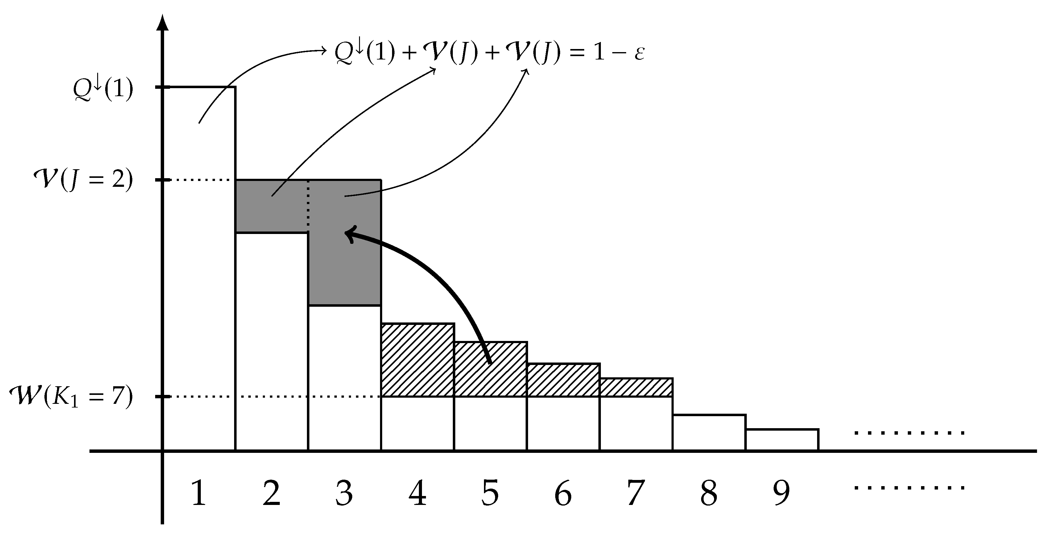
Figure 3.
Plot of making the extremal distribution of type-2 defined in (44) from an -marginal Q, where and . Each bar represents a probability mass of the decreasing rearrangement .
Figure 3.
Plot of making the extremal distribution of type-2 defined in (44) from an -marginal Q, where and . Each bar represents a probability mass of the decreasing rearrangement .

© 2020 by the author. Licensee MDPI, Basel, Switzerland. This article is an open access article distributed under the terms and conditions of the Creative Commons Attribution (CC BY) license (http://creativecommons.org/licenses/by/4.0/).
Share and Cite
MDPI and ACS Style
Sakai, Y. Generalizations of Fano’s Inequality for Conditional Information Measures via Majorization Theory. Entropy 2020, 22, 288. https://doi.org/10.3390/e22030288
AMA Style
Sakai Y. Generalizations of Fano’s Inequality for Conditional Information Measures via Majorization Theory. Entropy. 2020; 22(3):288. https://doi.org/10.3390/e22030288
Chicago/Turabian StyleSakai, Yuta. 2020. "Generalizations of Fano’s Inequality for Conditional Information Measures via Majorization Theory" Entropy 22, no. 3: 288. https://doi.org/10.3390/e22030288
Note that from the first issue of 2016, this journal uses article numbers instead of page numbers. See further details here.